Abstract
Accurate positioning of an airborne heavy-duty mechanical arm in coal mine, such as a roof bolter, is important for the efficiency and safety of coal mining. Its positioning accuracy is affected not only by geometric errors but also by nongeometric errors such as link and joint compliance. In this paper, a novel calibration method based on error limited genetic algorithm (ELGA) and regularized extreme learning machine (RELM) is proposed to improve the positioning accuracy of a roof bolter. To achieve the improvement, the ELGA is firstly implemented to identify the geometric parameters of the roof bolter’s kinematics model. Then, the residual positioning errors caused by nongeometric facts are compensated with the regularized extreme learning machine (RELM) network. Experiments were carried out to validate the proposed calibration method. The experimental results show that the root mean square error (RMSE) and the mean absolute error (MAE) between the actual mast end position and the nominal mast end position are reduced by more than 78.23%. It also shows the maximum absolute error (MAXE) between the actual mast end position and the nominal mast end position is reduced by more than 58.72% in the three directions of Cartesian coordinate system.
1. Introduction
Normally, an airborne heavy-duty mechanical arm has low positioning accuracy. “Airborne heavy-duty mechanical arm” is defined as a heavy-duty mechanical arm installed on a piece of coal mine machine. The coal mine machine is a high-voltage (1140 V/50 Hz) machine which uses hydraulic power to drive its mechanical arm. The coal mine machine can be a mining drill jumbo, a roof bolter, and a road header. The mining drill jumbo built by mining technologies international Inc. (MTI) has an airborne heavy-duty mechanical arm. The positioning accuracy of the MTI equipment is 50 mm [1]. The manipulators of a dual-arm rock drilling rig in [2] can also be considered as an airborne heavy-duty mechanical arm. Its positioning accuracy before calibration is 87 mm. In this paper, the heavy-duty mechanical arm of a roof bolter is studied. The positioning accuracy of the arm on the roof bolter is over 100 mm before calibration. Large positioning error not only degrades the quality of task, but also destroys equipment and brings fatal dangers to operators.
It is well known that the error sources of a mechanical arm can be classified into geometric errors and nongeometric errors. The geometric errors refer to nonperfect structure manufacturing, such as nonuniform link geometry and link twist. The nongeometric errors refer to the errors caused by joint and link compliance, gear backlash, and gear wear. Due to the heavy-duty characteristics of an airborne mechanical arm in coal mine, both types of errors have great impact on the performance of a coal mine machine.
Kinematics calibration is one of the most popular methods to improve the positioning accuracy of an industrial robot. By applying kinematics calibration, the positioning error caused by the link deformation can be compensated without changing the structure and links of an industrial robot. Much research on kinematics calibration has been reported in literature. In [3], Gao et al. proposed a parameter identification method based on Denavit–Hartenberg (DH) model. In [4,5,6,7], researchers studied the method of kinematics calibration based on the product of exponentials (POE) or improved POE model. In [8], Li et al. proposed an error model for serial robot kinematics calibration based on dual quaternions. The above mentioned research focused on modeling and geometric parameter error identification. However, these studies ignored the nongeometric errors, which are critical for positioning accuracy. Nongeometric errors cannot be ignored, especially when the equipment is heavy-duty.
There are few publications regarding the nongeometric error calibration. Chen et al. [9] proposed a rigid-flexible coupling error model for nongeometric calibration of a robot. In [10], Gong et al. established a comprehensive error model to identify the geometric errors, the position dependent compliance errors and time-variant thermal errors of an industrial robot. Some researchers [11,12] also established a comprehensive error model composed of geometric errors and compliance errors, and identified the geometric parameters and joint compliance of industrial robots. Owing to the difficulty of building an error model to include all nongeometric errors, most of the work in literature only took some nongeometric errors into consideration.
Thanks to its principle of data driven modeling, the artificial neural network (ANN) has a promising application in modeling complex systems such as calibration and error compensation of industrial robots [13,14,15,16]. However, one of the drawbacks of ANN for robot error calibration is the uncertainty of error sources. Therefore, Nguyen et al. [17] proposed a combination technique, which used extended Kalman filter (EKF) to identify the geometric errors and used the ANN to compensate the nongeometric errors. Similarly, Wang et al. [18] also proposed a combination method. In [18], the Denavit–Hartenberg (DH) model was applied to model and identify geometric errors. The nongeometric error sources, which are difficult to model, were compensated using ANN.
However, the training of an ANN is extremely slow. To overcome the limitation, Huang et al. [19,20] proposed an extreme learning machine (ELM) algorithm. Compared with the conventional ANN algorithm, ELM algorithm has faster learning speed and better generalization performance. ELM is a nonlinear system and can be used to compensate the unknown nonlinearity of robot nongeometric errors. Yuan et al. [21] proposed to improve the absolute positioning accuracy of an aviation drilling robot based on ELM. Although in [21] the implementation was easy, a user cannot obtain the source of geometric errors. Additionally, its performance will be less robust when outliers exist or when there are less training data. Deng et al. [22] proposed regularized extreme learning machine (RELM) based on empirical risk minimization (ERM) principle and structural risk minimization (SRM) principle. It turned out that RELM provided better generalization ability than ELM and run extremely fast like ELM.
In the current work, a novel calibration method is proposed to improve the positioning accuracy of the heavy-duty mechanical arm of a roof bolter in coal mine. This method is based on the combination of ELGA-based identification of the geometric errors and RELM-based residual errors compensation. The proposed method has the advantages of obtaining geometric error sources, high calibration efficiency, fast training speed, and good generalization performance.
The contributions of this paper are as follows:
- A method based on the combination of ELGA and RELM was proposed to solve the positioning error of the heavy-duty mechanical arm of a roof bolter in coal mine. It not only obtained the accurate knowledge of geometric error sources, but also compensates the nongeometric residual errors.
- The error-limited genetic algorithm (ELGA) is proposed to more accurately identify the optimal geometric parameters of the heavy-duty mechanical arm of a roof bolter. Compared with the conventional genetic algorithm, ELGA can converge to a better solution.
- The regularized extreme learning machine (RELM) is innovatively applied in residual positioning error compensation of the heavy-duty mechanical arm of a roof bolter in coal mine, which improves the speed of the positioning error calibration.
The rest of this paper is organized as follows: Section 2 provides the forward kinematics model for the identification of the geometric parameters. The error limited genetic algorithm (ELGA) and the principle of geometric parameter identification of the forward kinematics model are presented in Section 3, which is followed by the errors compensation principle based on RELM and constructs the RELM network in Section 4. Section 5 provides experimental setup and related results. The conclusion is given in Section 6.
2. Overview of the Problem
The actuation mechanism of a typical roof bolter is composed of a boom and a mast. The weight of each mast is about 2000 kg. In this paper, the goal is improving the positioning accuracy of the mast end position of a roof bolter.
Figure 1a shows the heavy-duty mechanical arm of a roof bolter and can function as a typical example of airborne heavy-duty mechanical arms in coal mine. Figure 1b shows the kinematics model of the airborne heavy-duty mechanical arm with six joints, which defines the coordinate system of each joint. {B} is the base coordinate system and {T} is the tool coordinate system. OB, O1, O2, O3, O4, O5, O6 and OT are the origin of coordinate system {B}, {1}, {2}, {3}, {4}, {5}, {6} and {T}, respectively. The origin OT of the tool coordinate system {T} is the mast end of a roof bolter.
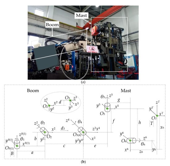
Figure 1.
A typical airborne heavy-duty mechanical arm: (a) the heavy-duty mechanical arm of a roof bolter; (b) the kinematics model of the airborne heavy-duty mechanical arm.
Each rotational joint of the mechanical arm takes the z axis as the rotation axis, where θ1, θ2, d3, θ4, θ5, θ6 are the motion variables of each joint around the z axis of the corresponding coordinate system, θ1 is the horizontal angle of the boom, θ2 is the vertical angle of the boom, d3 is the length of the boom, θ4 is the vertical angle of the mast, θ5 is the horizontal angle of the mast, and θ6 is the rotation angle of the mast around the z axis.
A homogeneous transformation from the {B} to the {T} coordinate system, which describes the position and pose of the mast end with respect to the base coordinate system {B}, is computed as Equation (1), where [Px, Py, Pz] is the position vector of the mast end relative to the base coordinate system {B}, [nx, ny, nz] is the direction cosine between the x axis of the tool coordinate system {T} and the x, y, z axis of the base coordinate system {B}, [ox, oy, oz] is the direction cosine between the y axis of the tool coordinate system {T} and the x, y, z axis of the base coordinate system {B}, [ax, ay, az] is the direction cosine between the z axis of the tool coordinate system {T} and the x, y, z axis of the base coordinate system {B}. Please refer to Appendix to obtain transformation matrix , (2 ≤ i ≤ 6) and [23].
3. Geometric Parameter Identification
3.1. Parameters to be Identified
The heavy-duty mechanical arm of a roof bolter, i.e., a particular drilling and anchoring robot, was used for parameter identification in order to illustrate better the principle. We define the actual position of the mast end measured using a laser tracker as Pr = [Pxr, Pyr, Pzr], the nominal position of the mast end calculated by kinematics model as Pm = [Pxm, Pym, Pzm], and the modified position of the mast end as P = [Px, Py, Pz].
As shown in Figure 1b, eleven geometric parameters a, b, c, d, e, f, g, h, x6, y6 and z6 are included in kinematics model, where x6, y6 and z6 can be measured as −1385 mm, −131 mm and 435 mm using the laser tracker. Therefore, eight geometric parameters of the kinematics model need to be identified. Initial values of eight geometric parameters are given according to the design parameters of the airborne heavy-duty mechanical arm structure. i.e., a = 230 mm, b = 139 mm, c = 2180 mm, d = 0 mm, e = 220 mm, f = −191 mm, g = 643 mm and h= −220 mm. The geometric parameters correction values of the kinematics model are mainly identified, and the geometric parameters to be identified are recorded as ∆a, ∆b, ∆c, ∆d, ∆e, ∆f, ∆g, and ∆h.
The problem of geometric parameter identification comes when finding a set of parameters ∆a, ∆b, ∆c, ∆d, ∆e, ∆f, ∆g, and ∆h, so that the difference between Pr and P is minimized. The root mean square error (RMSE) is used to evaluate the error reduction performance. This means that the objective function is RMSE. It is defined as Equation (2), where n is the number of training data. Because RMSE is a complex multivariable nonlinear function, the intelligent optimization genetic algorithm (GA) is implemented to solve it.
3.2. Error Limited Genetic Algorithm
A genetic algorithm (GA) is a stochastic search optimization algorithm. However, the conventional GA has the disadvantage of easy converging to the local optimal solution. An error-limited genetic algorithm (ELGA) with two improved strategies is proposed in this work. One strategy is to use a fitness function of error limited. The fitness function determines the evolution direction and efficiency of the algorithm. The other strategy is to use a catastrophe method after preserving an optimal solution to adjust the adaptive crossover probability threshold (PC) and the adaptive mutation probability threshold (PM) to fixed larger values. Using larger PC and PM produces more new individuals and can help escape local optimal solution. In each generation, an optimal solution larger than or equal to the previous generation is obtained. After many iterations, an optimal solution to meet the site requirement is achieved. As shown in Figure 2, ELGA’s improvements over GA are highlighted in blue.
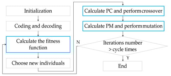
Figure 2.
Error-limited genetic algorithm (ELGA) flowchart.
As shown in Figure 2, Key steps of the ELGA are summarized as follows:
- Individual length which is the number of encoded bits in individual and population size are initialized. Then, the individuals of population are randomly generated. An individual contains eight parameters to be identified: Δa, Δb, Δc, Δd, Δe, Δf, Δg, and Δh.
- Each individual of the population is coded and decoded according to the multiparameter cascaded binary coding. The coding length is 55. Each of the eight parameters has a sign bit. Among them, Δa, Δe, Δf, Δg and Δh are coded using seven binary bits, Δb and Δd using six binary bits, and Δc using eight binary bits.
- The fitness function affects the convergence and stability of the ELGA. The linear function of the objective function RMSE is defined as the fitness function, as shown in Equation (3). For the commonly specified mining mesh of 50 mm × 50 mm, 50 mm × 100 mm, 100 mm × 100 mm and 100 mm × 200 mm, the positioning error of an airborne heavy-duty mechanical arm in coal mine should be less than 100 mm. The RMSE computed using Equation (2) can evaluate the positioning error. Therefore, the RMSE greater than or equal to 100 is useless. When the RMSE ≥ 100, the fitness function is set to 0, indicating the worst individual. According to the roulette wheel selection method, individuals with RMSE ≥ 100 (J = 0) is impossible to be selected and be passed on to the next generation. In this way, all individuals with RMSE ≥ 100 are excluded. The RMSE of retained individuals are less than 100. The individuals with RMSE < 100 are closer to the optimal solution than those with RMSE ≥ 100. Therefore, the evolution efficiency of Equation (3) as fitness function is higher.
- In order to keep the optimal solution, a combination of the roulette wheel selection method, and the elitism method is used to generate the selection operator. This means that, for the optimal individual, it is directly cloned to the next generation without roulette selection.
Crossover operation is the main step of generating new individuals in the ELGA. The single-point crossover operator is used in the crossover operation. A combination method of self-adaptive crossover probability threshold (PC) and catastrophe PC method is proposed. For N arbitrary individual, the PC value is calculated using Equation (4), where Jmax and Jmin represent the maximum and the minimum fitness function value in the population, respectively, flag is a Boolean variable indicating which will change PC and PM from adaptive values into fixed values, represents “not flag”. To illustrate the principle, a concept “the first optimal solution” is defined. “the first optimal solution” represents finding the first “the last iteration optimal solution Jmax” when the selection, crossover, mutation operations are performed during this iteration, flag = 0 means that “the first optimal solution” has not been found yet, flag = 1 indicates that the individual corresponding to “the first optimal solution” has been found and retained, after that, the fixed PC = 0.9 is used for crossover operation, the individual retained in the crossover operation is not taken as crossover object. The catastrophe method of using a larger PC generates a large number of new individuals.
The basic bit mutation operator is used in the mutation operation. Just as crossover, the mutation probability threshold (PM) is calculated using Equation (5):
- 5.
- If the termination condition is satisfied, exit the iteration and get an optimal solution to meet the site requirement. Otherwise, return to step 2.
4. RELM Compensation Principle
However, the geometric parameters identification using the ELGA does not eliminate the residual errors caused by nongeometric parameters. In this section, the residual errors compensation using the RELM with fast learning speed and good generalization ability is presented.
A single layer ELM network was used. The input weights and biases of the hidden layer are initialized randomly. These parameters do not need to be updated. Only the input weights of the output layer are to be obtained. The input weights of the output layer can be obtained by using Moore Penrose of the hidden layer output matrix [24]. ELM does not need iterative operation, which greatly improves the learning rate and generalization ability.
A three-layer ELM structure is shown in Figure 3. Pr = [Pxr, Pyr, Pzr] is the actual position measured using the laser tracker. Pm = [Pxm, Pym, Pzm] is calculated using the model before ELGA calibration. P = [Px, Py, Pz] is calculated using the model after ELGA calibration. The error E = [ex, ey, ez] between the actual position value Pr and the calibrated position value P is expressed as E = Pr − P.
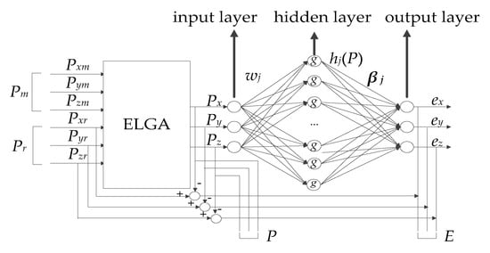
Figure 3.
Extreme learning machine (ELM) calibration model.
The three elements Px, Py and Pz of the position value P are three input nodes. The hidden layer consists of L neurons nodes. The error E is the output of the ELM. The three elements ex, ey and ez of the error E are three output nodes.
For N arbitrary samples {Pi, Ei | i = 1, …, N }, the output function of ELM is expressed as Equation (6):
where Pi = [Pxi, Pyi, Pzi]T is the input, Ei = [exi, eyi, ezi]T is the output, βj = [βxj, βyj, βzj]T represents the weight vector between the jth hidden node and the output nodes, hj(Pi) is the output function of the jth hidden point as expressed in Equation (7):
where g is a nonlinear activation function of hidden layer, sigmoid function is selected for g, wj = [wxj, wyj, wzj ]T is the weight vector between the jth hidden node and the input nodes, bj is the bias of the jth hidden node.
hj(Pi) = g(wjPi + bj), j = 1, …, L; i = 1, …, N,
In Equation (6), the N equations can be written compactly as Equation (8):
where
represents the weight matrix between hidden layer and output layer.
There are two steps to train the ELM network on the training data set. Firstly, input weights and biases of the hidden layer are generated randomly. The input data is mapped to a new feature space using Equation (7). Then, the weight matrix between hidden layer and output layer is calculated. When the number of samples is small, empirical risk minimization is likely to produce overfitting. According to the Bartlett’s theory [25], for the feedforward neural network with small training error, smaller weights norms leads to better network generalization performance. Deng et al. [22], Huang et al. [24] studied the RELM. The unweighted regularization objective function is used here, as in Equation (9):
where the first term is the least square error, i.e., the empirical risk, and the second term is the regularization term, i.e., the structural risk, > 0 is the parameter which balances the least square error and the regularization term. After a sixfold cross-validation experiment, was selected as 1. When the number of hidden nodes L is less than or equal to the number of training data, the solution is as Equation (10):
When the number of hidden nodes L is greater than the number of training data, the solution is as Equation (11):
After is calculated, testing data set is used to verify its effect.
5. Experiment and Results
5.1. Data Acquisition
Before the calibration, it is necessary to collect multiple data sets of the actual mast end position and the nominal mast end position. As shown in Figure 4, the measurement setup of the heavy-duty mechanical arm of a roof bolter consists mainly of a coordinate measuring machines (CMM), a laser tracker, and a target ball. The laser tracker made by Faro Vantage is a portable coordinate measuring instrument with a measuring space of thirty meters. The measurement accuracy of the laser tracker is: ±0.1 mm. The target ball was installed at mast end, which is the origin OT of the tool coordinate system. Based on the principle of laser reflection, the position of the target ball was tracked to obtain the absolute position of mast end.
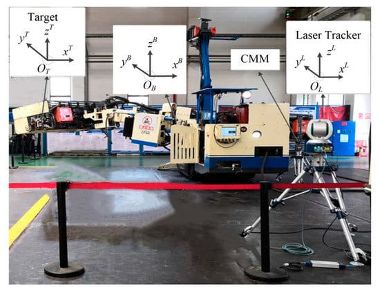
Figure 4.
The measurement setup of the heavy-duty mechanical arm of a roof bolter.
To help understand the measurement system, the base coordinate system (the origin OB), the laser tracker coordinate system (the origin OL), and the tool coordinate system (the origin OT) are highlighted in the picture. The absolute position of mast end in the base coordinate system can be obtained using Equation (12). Where, the linear transformation was measured using the CMM, the linear transformation was measured using the laser tracker.
In the data collection experiments, the target ball was navigated to 80 positions evenly distributed in the working space. For each position, joint angles and the length of the boom are obtained by sensors, the controller calculated a position according to the forward kinematics model and sensors reading, which is the nominal mast end position. Meanwhile, the measurement software also calculated a position to match the laser tracker measurement, which was considered as the actual mast end position. We repeated the test six times and ran 80 positions each time to obtain a total of 480 data. We selected 360 data for this study, where 300 of the data was used as training data and 60 of the data was used as testing data to verify the calibration effect.
5.2. Positioning Calibration Experiment
In order to verify the effect of the proposed positioning error calibration method, experiments were carried out on the heavy-duty mechanical arm of a roof bolter. The validation experiment was conducted in two steps. The first step is parameter identification. The second step is residual positioning error compensation.
5.2.1. Parameter Identification
According to the step-by-step improvement process of GA algorithm, the first three steps were three experiments considering three cases. The last step is to verify that the optimal solution obtained by the third step experiment and approximate global optimal solution can achieve similar calibration accuracy. The iteration number was set to 50 in all cases. In Figure 5a–c, the population size was set to 30. In Figure 5d, the population size was set to 1000. Experiments were conducted 30 times for the four cases, respectively. A representative experiment was selected.
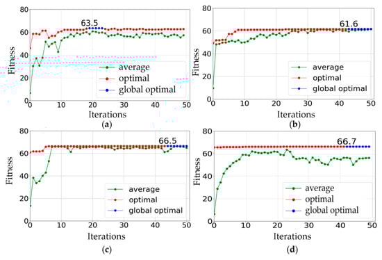
Figure 5.
The ELGA experiments: (a) genetic algorithm (GA) with PC (crossover probability threshold) = 0.9, PM (mutation probability threshold) = 0.1 and without elitism; (b) GA with PC = 0.9, PM = 0.1 and with elitism; (c,d) A combination of self-adaptive and catastrophe PC, PM; (c) Population size = 30, running time = 114.0 s; (d) Population size = 1000, running time = 4164.3 s.
In Figure 5, “average” is the average fitness value of all individuals in each iteration in a run, “optimal” is the maximum fitness value of all individuals in each iteration in a run and “global optimal” is the maximum value of “optimal” in all iterations in a run.
In Figure 5a, the GA with fixed PC and fixed PM without elitism was implemented. The optimal fitness function did not keep growing, which means no convergence during operation. The problem in Figure 5a was improved using the GA with elitism. However, in Figure 5b, the phenomenon of falling into local optimal occurred. In Figure 5c, self-adaptive PC, self-adaptive PM and catastrophe method were combined to solve this problem. The optimal fitness value was 66.5 and the running time was 114.0 s.
In Figure 5d, the population size was changed to 1000. The experiment took 4164.3 s to converge to 66.7. The optimal solutions when the population sizes were 30 and 1000 can achieve similar calibration accuracy. However, when the population size was 1000, it took more than 30 (4164.3 s/114.0 s = 36.53) times longer than when the population size was 30. It is concluded that the proposed method solved the problem of falling into local optimal with a small population size and obtained an optimal solution which has the most approximate calibration effect with the global optimal solution.
When population size = 30 and iterations number = 50, the statistical results of 30 experiments are shown in Figure 6, the individual with a fitness function value of 66.474 was selected as the optimal individual. The corresponding correction parameters vector is (∆a, ∆b, ∆c, ∆d, ∆e, ∆f, ∆g, ∆h) = (52.0, −8.0, −58.0, 31.0, 15.0, 16.0, 49.0, −2.0). The geometric parameters of the updated kinematics model are shown in Table 1.
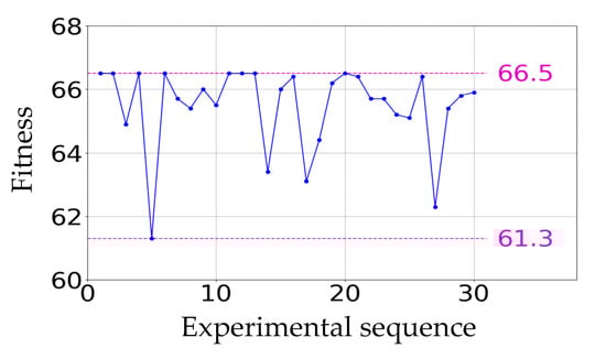
Figure 6.
The statistical results of 30 ELGA experiments: population size = 30, iterations number = 50.

Table 1.
The updated geometric parameters of the kinematics model.
5.2.2. Residual Positioning Error Compensation
Selection of Hidden Nodes in ELM Network
The maximum absolute error (MAXE) is an important index in positioning error calibration. The root mean square (RMS) of the x, y and z directions’ MAXEs in the ith network is RMSMAXE-i, as shown in Equation (13):
where xMAXE-i is the average value of the x direction MAXEs of 20 experiments in the ith network, yMAXE-i and zMAXE-i are similar to xMAXE-i.
The smaller RMSMAXE-i, the smaller the x, y and z directions MAXEs. In order to minimize the MAXE in all directions, the number of hidden nodes of ELM network was selected using the RMSMAXE-i. In general, the training time increases with the number of hidden nodes in ELM network, so training time is also used as an optimal criterion.
Twenty different networks with the number of hidden nodes range from 10 to 200 had been experimentally evaluated on training data set. Twenty experiments were conducted for each network. The simulation experiments were carried out in MATLAB environment running on a windows computer with a 2.60-GHz Intel Core i7-9750H CPU (Intel, Santa Clara, CA, USA) and 16.0 GB RAM. As shown in Figure 7a, as the number of hidden nodes was less than 70, the RMS of x, y and z directions MAXEs reduced as the number of hidden nodes increased. When the number of hidden nodes was more than 70, the RMS of the x, y and z directions MAXEs tended to be stable, but when the number of hidden nodes was 140, the RMS of the x, y and z directions MAXEs was the smallest.
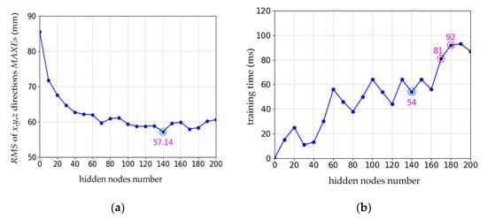
Figure 7.
Selection of hidden nodes: (a) effect of maximum absolute error (MAXE) on hidden nodes number; (b) effect of training time on hidden nodes number.
The training time average value of 20 experiments is taken. As shown in Figure 7b, with the increase of hidden nodes, the training time of ELM network goes up in a zigzag way. When the number of hidden nodes was 140, the training time of ELM network was 54 ms, which is similar to the operation time of hidden nodes between 60 and 160. When the number of hidden nodes was greater than or equal to 170, the operation time was greater than 81 ms. Considering the smaller RMS of x, y and z directions MAXEs and less training time, a network of 140 hidden nodes is selected to compensate the residual positioning errors.
As shown in Figure 7b, in the 20 different networks with the number of hidden nodes range from 10 to 200, the training time was always less than 100 ms, so the training speed of ELM network is fast.
Selection of Activation Functions
Nonlinear piecewise continuous functions, such as sigmoid and Gaussian, can be selected as the activation functions of ELM network. The comparison experiment is carried out here. In the comparison experiment, number of nodes in hidden layer is 140. Gaussian function, radial basis function, tanh function and sigmoid function are selected as activation functions.
In Table 2, Gaussian (0,1) means the expectation of Gaussian function is 0 and the variance is 1, Gaussian (2,1) means the expectation of Gaussian function is 2 and the variance is 1. For each case, 20 experiments were done. The average training time, RMSE, RMSE_x, RMSE_y and RMSE_z are shown in Table 2. Table 2 shows that RMSEs are larger when Gaussian function and radial basis function are used as activation functions. When sigmoid and tanh are used as activation functions, RMSEs are smaller. However, the training time using tanh function is slightly longer than sigmoid. Therefore, sigmoid function is suitable for activation function in this research.
Table 2.
Comparison experiments using different activation functions on training data set.
Selection of RELM Network
In this section, the two types of objective functions with and without regularization term in ELM networks were compared, as shown in Table 3. For each network, 30 experiments were done and the over fitting phenomenon was counted. In Table 3, 2/30 indicates that over fitting occurred twice in 30 experiments. The result showed that over fitting became worse and worse with the increasing number of hidden nodes when objective function has not a regularization term. However, there was no overfitting phenomenon when the objective function had a regularization term. Therefore, the objective function with regularization term was selected.
Table 3.
Statistics of over fitting times.
ELGA-RELM Experiment
The ELGA-RELM model was established by doing experiments on training data set, and the effect of positioning error calibration was verified on testing data set.
We list the RMSE, the MAE and the MAXE of the evaluation in Table 4. The positioning error reduction on testing data set was about the same as on training data set. It can be seen that the MAXEs were reduced from more than 100 mm to less than 29.54 mm in the x, y and z directions, from the result, the proposed calibration method can meet the positioning accuracy requirement of mesh support in coal mine.
Table 4.
The positioning error evaluations of on testing data set.
Figure 8a shows the positioning error before the kinematics model was updated on testing data set. Figure 8b shows the positioning error after the geometric parameters of the kinematics model were identified using ELGA. The absolute position error was reduced from nearly 100 mm to less than 50 mm in the x, y and z directions. Figure 8c shows that the absolute positioning error was reduced from nearly 50 mm to less than 30 mm after the nongeometric residual error was compensated using RELM.
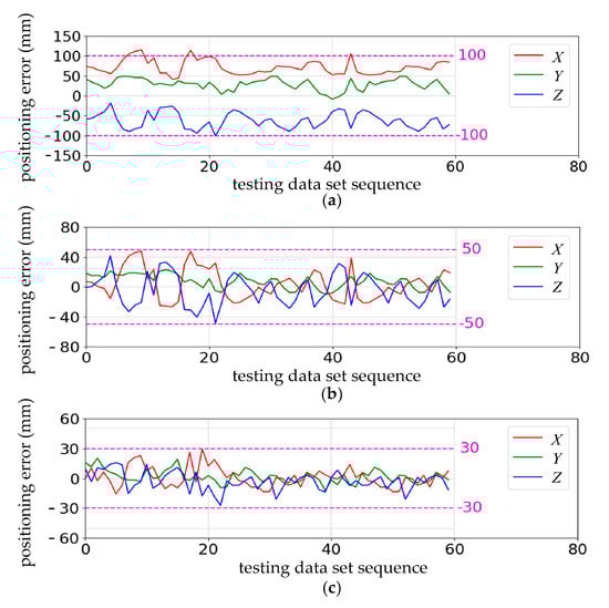
Figure 8.
Positioning error contrast diagram on testing data set: (a) before calibration; (b) after the kinematics model was updated; (c) after the residual error was compensated.
Comparison of back propagation (BP), ELM and RELM
In order to verify the validity of RELM network in positioning error calibration, we compared RELM with the ELM and BP networks. The BP network is a sort of typical forward ANN. Twenty experiments were done and the average results were obtained. As observed from Table 5, RELM had better generalization performance than ELM. The training time of BP is 30 times more than that of RELM. The RMSE of BP and RELM is close. Therefore, RELM is more suitable for the positioning error calibration of an airborne heavy-duty mechanical arm.
Table 5.
Comparison of back propagation (BP), extreme learning machine (ELM) and regularized extreme learning machine (RELM).
5.3. Validation Experiment
In order to verify the performance on site of proposed method, an automatic positioning experiment of the heavy-duty mechanical arm of a roof bolter was carried out. Figure 9 shows the process of an automatic positioning cycle. This process mainly realized the positioning of three bolting positions. Figure 9a,i are the heavy-duty mechanical arm of a roof bolter initial position. Figure 9c,e,g are the three bolting positions, the rest of the Figure 9 show the process of moving to the next bolting position. After the mast end moved to three bolting positions by following the set trajectory, the mast finally returned to its initial position.
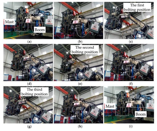
Figure 9.
Automatic positioning process: (a,i) initial position; (c) the first bolting position; (e) the second bolting position; (g) the third bolting position; (b,d,f) the process of moving to the next bolting position; (h) the process of returning to the initial position.
The RMSE, MAE and MAXE of the experiment are listed in Table 6. It can be seen that the MAXEs were reduced to 34.35 mm in the x, y and z directions. The results further show that the proposed calibration method can meet the positioning accuracy requirements of a 50 mm × 50 mm mesh support used in coal mine.
Table 6.
The positioning error evaluations of validation experiment.
In the experiment, the mast end was commanded to follow a “III” shape trajectory. The result is shown as the three-dimensional graph in Figure 10d. Figure 10a–c represent the mast end motion curve in the y, z and x directions, respectively. In Figure 10, the red curve represents the track before calibration. The purple curve represents the track after the kinematics model are identified using ELGA. The green curve represents the track after ELGA-RELM calibration. The blue curve represents the actual mast end position. A total of 100 positions of the trajectory were collected in the experiment. It can be seen that the purple, green and blue tracks are close, and green track was almost coincident with the blue track in Figure 10, which proved that the errors after calibration were significantly reduced with the proposed calibration method in this paper.
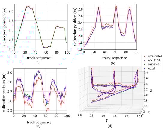
Figure 10.
The “III” shape trajectory:(a) the motion curve in the y direction; (b) the motion curve in the z direction; (c) the motion curve in the x direction; (d) three-dimensional graph of the trajectory. In (a)–(c) The horizontal axis represents the track sequence number obtained according to the routing order.
6. Conclusions
In this paper, a novel calibration method based on error-limited genetic algorithm (ELGA) and regularized extreme learning machine (RELM) was proposed to improve the positioning accuracy of an airborne heavy-duty mechanical arm. The novel calibration method has many advantages, such as obtaining geometric error sources, less training time, good generalization ability, and good error calibration effect.
The heavy-duty mechanical arm of a roof bolter was studied in this work to prove the proposed positioning calibration method. We first used the sensors on the equipment, combining with the forward kinematics model, to calculate the nominal mast end position. Then, we used a laser tracker to measure the actual mast end position. Based on the calculated and the measured positions, a root mean square error equation was established. The geometric parameters of the error equation were identified and optimized using the ELGA. Finally, the kinematics model was updated.
Based on the updated kinematics mode, further residual error compensate was carried out using a RELM network. After error compensation with RELM, the RMSEs, MAEs and MAXEs on testing data set were reduced by more than 78.23%, 81.35%, and 58.72% respectively. The maximum absolute errors (MAXEs) in the x, y and z directions were reduced to less than 29.54 mm. It indicates that the method proposed in this paper can meet the support accuracy requirements of the 50 mm × 50 mm mesh for a roof bolter in coal mine. It was further proved in the validation experiment.
Author Contributions
Y.J. carried out the main research tasks, wrote the manuscript and analyzed the data; Z.W. and X.Z. contributed the analysis method; Y.J. and W.W. designed and carried out the numerical experiments; W.W. designed the structure of the heavy-duty mechanical arm of a roof bolter. All authors have read and agreed to the published version of the manuscript.
Funding
This research was funded by the National Development and Reform Commission of China under grant No. 1371[2018]; the ShanXi Province Science Fund under grant No.201801D121189; the Science and Technology Innovation of TianDi Science and Technology Co., Ltd. of China under grant No. 2018-TD-MS040, and No.2018-TD-MS042; the Key R & D plan of ShanXi Province under grant No. 201903D121076.
Conflicts of Interest
The authors declare no conflict of interest.
Appendix
Transformation matrix , (2 ≤ i ≤ 6) and can be obtained from the position relationship of each coordinate system in Figure 1 [23].
where [a, b, c, d, e, f, g, h, x6, y6, z6] is a vector containing all the kinematics geometric parameters, and are short forms of and , respectively.
References
- Wang, Y.J.; Fang, C.; Jiang, Q.M.; Ahmed, S.N. The automatic drilling system of 6R-2P Mining Drill Jumbos. Adv. Mech. Eng. 2015, 7, 504861. [Google Scholar] [CrossRef]
- Xie, X.H.; Li, Z.Y.; Wang, G. Manipulator calibration based on PSO-RBF neural network error model. AIP Conf. Proc. 2019, 2073, 19–20. [Google Scholar]
- Gao, G.B.; Sun, G.Q.; Na, J.; Guo, Y.; Wu, X. Structural parameter identification for 6 DOF industrial robots. Mech. Syst. Signal. Process. 2018, 113, 145–155. [Google Scholar] [CrossRef]
- Chang, C.G.; Liu, J.G.; Ni, Z.Y.; Qi, R.L. An improved kinematic calibration method for serial manipulators based on POE formula. Robotica 2018, 36, 1244–1262. [Google Scholar] [CrossRef]
- Liu, H.; Zhu, W.D.; Dong, H.Y.; Ke, Y.L. An Improved kinematic model for serial robot calibration based on local POE formula using position measurement. Ind. Robot Int. J. Robot. Res. App. 2018, 45, 573–584. [Google Scholar] [CrossRef]
- He, R.B.; Li, X.W.; Shi, T.L.; Wu, B.; Zhao, Y.J.; Han, F.L.; Yang, S.N.; Huang, S.H.; Yang, S.Z. A kinematic calibration method based on the product of exponentials formula for serial robot using position measurements. Robotica 2015, 33, 1295–1313. [Google Scholar] [CrossRef]
- He, R.B.; Zhao, Y.J.; Yang, S.N.; Yang, S.Z. Kinematic-parameter identification for serial-robot calibration based on POE formula. IEEE. Trans. Robot. 2010, 26, 411–423. [Google Scholar]
- Li, G.Z.; Zhang, F.H.; Fu, Y.L.; Wang, S.G. Kinematic calibration of serial robot using dual quaternions. Ind. Robot Int. J. Robot. Res. App. 2019, 46, 247–258. [Google Scholar] [CrossRef]
- Chen, X.Y.; Zhang, Q.J.; Sun, Y.L. Non-kinematic calibration of industrial robots using a rigid-flexible coupling error model and a full pose measurement method. Robot. Comput. Integr. Manuf. 2019, 57, 46–58. [Google Scholar] [CrossRef]
- Gong, C.H.; Yuan, J.X.; Ni, J. Nongeometric error identification and compensation for robotic system by inverse calibration. Int. J. Mach. Tool. Manu. 2000, 40, 2119–2137. [Google Scholar] [CrossRef]
- Zhou, J.; Nguyen, H.N.; Kang, H.J. Simultaneous identification of joint compliance and kinematic parameters of industrial robots. Int. J. Precis. Eng. Man. 2014, 15, 2257–2264. [Google Scholar] [CrossRef]
- Zhou, J.; Kang, H.J. A Hybrid Least-squares genetic algorithm–based algorithm for simultaneous identification of geometric and compliance errors in industrial robots. Adv. Mech. Eng. 2015, 7, 1–12. [Google Scholar] [CrossRef]
- Wang, D.L.; Bai, Y.; Zhao, J.Y. Robot manipulator calibration using neural network and a camera-based measurement system. Trans. Meas. Control. 2012, 34, 105–121. [Google Scholar] [CrossRef]
- Jang, J.H.; Kim, S.H.; Kwak, Y.K. Calibration of geometric and non-geometric errors of an industrial robot. Robotica 2001, 19, 311–321. [Google Scholar] [CrossRef]
- Cao, C.T.; Do, V.P.; Lee, B.R. A novel indirect calibration approach for robot positioning error compensation based on neural network and hand-eye vision. Appl. Sci. 2019, 9, 1940. [Google Scholar] [CrossRef]
- Su, H.; Qi, W.; Hu, Y.B.; Sandoval, J.; Zhang, L.B.; Schmirander, Y.; Chen, G.; Aliverti, A.; Knoll, A.; Ferrigno, G.; et al. Towards model-free tool dynamic identification and calibration using multi-layer neural network. Sensors 2019, 19, 3636. [Google Scholar] [CrossRef]
- Nguyen, H.N.; Zhou, J.; Kang, H.J. A calibration method for enhancing robot accuracy through integration of an extended kalman filter algorithm and an artificial neural network. Neurocomputing 2015, 151, 996–1005. [Google Scholar] [CrossRef]
- Wang, Z.R.; Chen, Z.W.; Wang, Y.X.; Mao, C.T.; Hang, Q. A robot calibration method based on joint angle division and an artificial neural network. Math. Probl. Eng. 2019, 2019, 9293484. [Google Scholar] [CrossRef]
- Huang, G.B.; Zhu, Q.Y.; Siew, C.K. Extreme learning machine: Theory and applications. Neurocomputing 2006, 70, 489–501. [Google Scholar] [CrossRef]
- Deng, C.W.; Huang, G.B.; Xu, J.; Tang, J.Q. Extreme learning machines: New trends and applications. Sci. China. Inf. Sci. 2015, 58, 1–16. [Google Scholar] [CrossRef]
- Yuan, P.J.; Chen, D.D.; Wang, T.M.; Cao, S.Q.; Cai, Y.; Xue, L. A compensation method based on extreme learning machine to enhance absolute position accuracy for aviation drilling robot. Adv. Mech. Eng. 2018, 10, 1–11. [Google Scholar] [CrossRef]
- Deng, W.Y.; Zheng, Q.H.; Chen, L. Regularized extreme learning machine. In Proceedings of the 2009 IEEE Symposium on Computational Intelligence and Data Mining, Nashville, TN, USA, 30 March–2 April 2009; Volume 2, pp. 389–395. [Google Scholar]
- Guo, Z.F. Research on Spatial Pose and Collision Detection Technology of Automatic Dual-Arm Bolter. Ph.D. Thesis, China University of Mining and Technology (Beijing) & Shenhua Shendong Coal Group Co., Ltd., Beijing, China, 2017. [Google Scholar]
- Huang, G.B.; Zhou, H.M.; Ding, X.J.; Zhang, R. Extreme learning machine for regression and multiclass classification. IEEE. Trans. Syst. Man. Cybern. Part B Cybern. 2012, 42, 513–529. [Google Scholar] [CrossRef] [PubMed]
- Bartlett, P.L. The sample complexity of pattern classification with neural networks: The size of the weights is more important than the size of the network. IEEE. Trans. Inf. Theory 1998, 44, 525–536. [Google Scholar] [CrossRef]
© 2020 by the authors. Licensee MDPI, Basel, Switzerland. This article is an open access article distributed under the terms and conditions of the Creative Commons Attribution (CC BY) license (http://creativecommons.org/licenses/by/4.0/).