Article

Adaptive Weighted High Frequency Iterative Algorithm for Fractional-Order Total Variation with Nonlocal Regularization for Image Reconstruction

Institute of Fiber-optic Communication and Information Engineering, College of Information Engineering, Zhejiang University of Technology, Hangzhou 310023, China
*
Author to whom correspondence should be addressed.
Electronics 2020, 9(7), 1103; https://doi.org/10.3390/electronics9071103
Submission received: 17 June 2020 / Revised: 30 June 2020 / Accepted: 1 July 2020 / Published: 7 July 2020
(This article belongs to the Special Issue Theory and Applications in Digital Signal Processing)

Abstract

:
We propose an adaptive weighted high frequency iterative algorithm for a fractional-order total variation (FrTV) approach with nonlocal regularization to alleviate image deterioration and to eliminate staircase artifacts, which result from the total variation (TV) method. The high frequency gradients are reweighted in iterations adaptively when we decompose the image into high and low frequency components using the pre-processing technique. The nonlocal regularization is introduced into our method based on nonlocal means (NLM) filtering, which contains prior image structural information to suppress staircase artifacts. An alternating direction multiplier method (ADMM) is used to solve the problem combining reweighted FrTV and nonlocal regularization. Experimental results show that both the peak signal-to-noise ratios (PSNR) and structural similarity index (SSIM) of reconstructed images are higher than those achieved by the other four methods at various sampling ratios less than 25%. At 5% sampling ratios, the gains of PSNR and SSIM are up to 1.63 dB and 0.0114 from ten images compared with reweighted total variation with nuclear norm regularization (RTV-NNR). The improved approach preserves more texture details and has better visual effects, especially at low sampling ratios, at the cost of taking more time.

1. Introduction

Compressed sensing (CS) [1,2] is an emerging framework for data acquisition and reconstruction, which permits us to reconstruct the original sparse or compressible signals from only a small number of linear measurements. CS has been exploited in image processing, such as 3D video [3], medical imaging [4], single-pixel imaging [5]. This is based on the principle that, through optimization, the sparsity of a signal can be recovered from far fewer samples than required by the Nyquist–Shannon sampling theorem when the measurement matrix satisfies the restricted isometry property (RIP) [6]. There is an attractive advantage that CS-based methods decrease data storage and transmission costs significantly for systems requiring large data. The most notable application, the single-pixel imaging system, reconstructed images from only a small amount of data from a single photodetector, with the result that it implements the mixing of image signals with a random mask such as the Hadamard matrix generated by a digital micromirror device (DMD) [7].
More specifically, the CS model reconstructs the image x R n from measurements y and it can be expressed as:
min x Ψ x   s . t .   y = A x
where Ψ is transformation domain, A R M × N represents measurement matrices. The image x can be recovered by an inverse problem:
x ^ = argmin x 1 2 A x y 2 2 + μ Ψ ( x )
where Ψ ( x ) is a sparse prior, μ is the regularization parameter, which can control the trade-off between the regularization and data fidelity. Sparse prior knowledge [8] plays an important role in signal reconstruction. Generally, the current CS algorithms exploit the prior knowledge of original images under some suitable transformation such as DCT [9], wavelets [10], and total variation model [11,12]. The most popular approach is TV owing to the advantages of preserving image edges and reconstruction performance, which can be defined as:
x T V = i = 1 n ( D x x i ) 2 + ( D y x i ) 2
where D x and D y denote horizontal and vertical difference operators, respectively.
TV models sets the same penalty for all gradients, which fails to preserve image details accurately and often leads to undesirable serious staircase artifacts. So many improved solvers have been proposed such as TVAL3 [13], TVNLR [14], RTV-NNR [15]. Li CB et al. proposed TVAL3, introducing an augmented Lagrangian method and an alternating technique with a nonmonotone line search to preserve edges. Zhang et al. [14] used an improved nonlocal regularization constraint operator, reducing reconstruction errors significantly by averaging the weights of TV regularization. Candes [16] proposed a reweighted TV, which penalized the gradients in each iteration adaptively with the weights w i . The model can be expressed as:
x R T V = i = 1 n w i ( D v x i ) 2 + ( D h x i ) 2
where weights w can be defined as:
w i t + 1 = 1 D x i t 2 + ε
Weights w are updated by x in each iteration, setting the different penalty for different regions. The parameter ε is a small positive constant to avoid division by zero. The regions which have large gradients (e.g., texture details) have small penalty and the others have large penalty. This method preserves the image edges effectively.
To improve the quality of reconstructed images, another strategy is nonlocal regularization based on nonlocal means (NLM) filtering. This strategy is effective for preserving image details and sharp edges by exploiting structural information. Dong [17] proposed a nonlocal low-rank regularization method using a smooth surrogate function for the rank as structured sparsity instead of the convex nuclear norm. This method combines nonlocal self-similarity and low rank to eliminate redundant information and artifacts. However, the reconstructed images are over-smoothed owing to the average tendency of different similar patches.
In this paper, we propose an adaptive reweighted fractional-order TV with nonlocal regularization for image reconstruction. This approach improves the TV model and only weights the high frequency gradients by extracting the high frequency components (e.g., texture details) from the images using pre-processing technique [18]. Fractional-order differential operators are introduced into the TV model replacing integer-order differential operators, enhancing high frequency components of images. We adopted the Grünwald–Letnikov (G-L) model using four different directions to handle the fractional-order gradients. Prior knowledges are exploited by introducing the nonlocal regularization constraint as structural information. An efficient augmented Lagrangian is developed to solve the above problem. ADMM is used to decompose this objective function into four sub-problems. We evaluate reconstruction performance by using peak a signal-to-noise (PSNR) and structural similarity index (SSIM) compared with other TV-based CS reconstruction methods.
We decompose the low and high frequency components, analyze the fractional differential model with different directions and give the definitions of nonlocal regularization in Section 2 of this paper. In Section 3, we describe equations of the proposed models. In Section 4, experimental results demonstrate the effectiveness of the proposed models. In Section 5, we give the conclusion.

2. Related Works

2.1. Fractional-Order Differential Model

We introduce a fractional-order differential operator into TV-based algorithm. A fractional-order gradient, regarded as a generalization of the integer-order gradient, is composed of the fractional-order derivative at different directions. Here, we use the Grünwald–Letnikov (G-L) model [19,20] for image reconstruction and this model can be defined as:
D a G t v f ( x ) = lim h 0 1 h v k = 0 [ t a h ] ( 1 ) m × C k v × f ( t k h )
where v is fractional orders of function, t and a are the upper and lower boundaries of independent variables respectively, and h is the differential step-size.
The total variation model of the image X can be viewed as the sum of two-dimensional discrete signal gradients in Equation (3). Fractional-order differential operators are introduced into the TV model, and the new model can be expressed as:
v x F T V = ( D x v x ) 2 + ( D y v x ) 2
where D x v , D y v represent fractional-order gradients in horizontal and vertical directions respectively:
{ D x v x = k = 0 k 1 ( 1 ) k C k v x i k , j D y v x = k = 0 k 1 ( 1 ) k C k v x i , j k
More specifically, we use four different directions to handle fractional-order gradients simply, corresponding to negative x and y axes, positive x and y axes, which the approximate extensive backward difference and the forward difference can be deduced easily. If the higher accuracy is required, more different directions (i.e., eight directions or sixteen directions) can be used with time costs permitting. In Equation (8), the corresponding coefficients C k v are expressed as:
{ C 0 v = 1 C 1 v = v C 2 v = v ( v 1 ) 2 C k v = ( 1 ) k Γ ( v + 1 ) Γ ( k + 1 ) Γ ( v k + 1 )
According to Equation (9), four different expressions can be written as:
D x v = C 0 v x i , j + C 1 v x i 1 , j + C 2 v x i 2 , j + + C k 1 v x i k + 1 , j D y v = C 0 v x i , j + C 1 v x i , j 1 + C 2 v x i , j 2 + + C k 1 v x i , j k + 1 D x + v = C 0 v x i , j C 1 v x i + 1 , j C 2 v x i + 2 , j C k 1 v x i + k 1 , j D y + v = C 0 v x i , j C 1 v x i , j + 1 C 2 v x i , j + 2 C k 1 v x i , j + k 1
The fractional differential model enhances high frequency components more effectively, which preserves image details meanwhile losing some low frequency components.

2.2. Adpative Reweighted Total Variation Model

Natural images can be decomposed into smooth regions (low frequency components) and texture details (high frequency components), such as Lena in Figure 1. There is a fuzzy contour in Figure 1a, and it contains the most of image energy. Sharp edge textures can be seen in Figure 1b, which is crucial for visual effects. Equation (4) sets the different penalty for different gradients to preserve image edges without considering the structural information that results in the false textures and artifacts.
We propose a new adaptive reweighting strategy for total variation model to solve the problem which loses the high frequency parts of the images. Decomposing low and high frequency components is a critical technique for the new strategy. Image x is decomposed into the smooth regions (low frequency) x L and image details (high frequency) x H . We only weight the high frequency components x H in iterations. The new TV model can be defined as:
>x R T V = i x L | D i >x L | + i >x H w i | D i x H |
To extract the low frequency components of images, we can solve the following deconvolution problem:
arg min Z L 1 2 x f L Z L 2 2 + κ d g d Z L 2 2
where f L is a 3 × 3 low pass filter and all coefficients are 1 / 9 , denotes convolution operation. Z L is a low frequency feature map, and g d = [ 1 , 1 ] is the horizontal and vertical gradient operator. κ is a user-defined parameter. The solution of Equation (12) can solved by fast Fourier transform (FFT):
Z L = 1 ( ( f L ) ( x ) ( f L ) ( f L ) + κ d ( g d ) ( g d ) )
where and 1 is FFT and inverse FFT, ‘ ’ denotes complex conjugate, and ‘ ’ denotes component-wise multiplication.
Therefore, the low and high frequency components can be expressed as:
{ x L = f L Z L x H = x x L
We only employ the high frequency components to update the weights:
w i t + 1 = 1 x H t 2 2 + ε

2.3. Nonlocal Regularization Model

For nature images, there are lots of same image patches in different regions and the same patches may be far apart in space domain, that is the nonlocal similarity. The similarity between two patches depends on the similarity of intensity gray levels by measuring Gaussian weighted Euclidean distances. We consider a nonlocal regularization model [21,22] based on nonlocal self-similarity to obtain more appropriate weight coefficients.
Given an image x = { x ( i ) | i Ω } , the estimate value x ^ ( i ) for a pixel i can be defined as:
x ^ ( i ) = j S ( i ) ω i j x ( j )
where S ( i ) is a i-centered search window L s × L s , x ( j ) is the intensity at pixel j. N i and N j denote the center pixel of similarity window d s × d s . The weights w i j depending on the similarity between gray value vectors P ( N i ) and P ( N j ) , can be defined as:
W ( i , j ) = ω i j = 1 Z ( i ) exp ( P ( N i ) P ( N j ) 2 , α 2 / h 2 )
where h is an attenuation factor, altering the decay of the exponential function, and α is a standard deviation for Gaussian kernels. Z ( i ) is a normalizing constant, defined as:
Z ( i ) = j exp ( P ( N i ) P ( N j ) 2 , α 2 / h 2 )
The nonlocal regularization (NR) model is expressed as:
N R ( x ) = x W x 2 2

3. Reweighted Fractional-Order TV Method with Nonlocal Regularization

In this section, we consider two strategies to improve the TV method for solving texture deficiency. First, low frequency and high frequency components of images are decomposed by Equations (13) and (14). Fractional differential operators are introduced into the TV model by using four different directions to handle fractional-order gradients approximately. We defined the FrTV weights by using Equation (15) and only adaptively reweight the high frequency gradients. Second, the nonlocal regularization constraint is employed as structural information to eliminate staircase artifacts.
The proposed method can be expressed as the optimization problem:
arg min x 1 2 A x y 2 2 + λ { | D v x L | + w | D v x H | } + β ( I W ) x 2 2
where λ and β are regularization parameters, w is the high frequency parts weights and W is a regularization matrix. It is difficult to solve directly due to the non-differentiability. To solve this problem efficiently, we add constrained auxiliary variables:
arg min x 1 2 A x y 2 2 + λ { | Z L | + w | Z H | } + β ( I W ) u 2 2 s . t . x = u , D v x L = Z L , D v x H = Z H
The corresponding augmented Lagrangian converting constrained Equation (21) into unconstrained objective functions:
( u , x , Z L , Z H ) = arg min x 1 2 A x y 2 2 + λ { | Z L | + w | Z H | } + β ( I W ) u 2 2 + α 2 u x + a 2 2 + γ 1 2 Z L D v x L + b 2 2 + γ 2 2 Z H D v x H + c 2 2
where a, b, c are the Lagrangian multipliers, α , γ 1 , γ 2 are corresponding meta-parameters. We solve the Equation (22) by solving Equations (23) and (24) iteratively:
( u t + 1 , x t + 1 , Z L t + 1 , Z H t + 1 ) = arg min u , x , Z L , Z H ( u t , x t , Z L t , Z H t )
{ a t + 1 = a t ( x t + 1 u t + 1 ) b t + 1 = b t ( D v x L t + 1 Z L t + 1 ) c t + 1 = c t ( D v x H t + 1 Z H t + 1 )
Alternating direction method of multipliers (ADMM) is drawn into decomposing four sub-problems using a variable splitting technique. We update each parameter iteratively until convergence. Assuming other parameters are fixed, u problem can be expressed as:
u t + 1 = arg min u β ( I W ) u 2 2 + α 2 u x t + a t 2 2
Equation (25) has the closed form solution. Derivative Equation (25) and make derivative zero, we can obtain the solution:
u t + 1 = α [ β ( I W ) T ( I W ) + α I ] 1 ( x t a t )
Fixing u, x, Z H , the sub-problem Z L is equivalent to:
Z L t + 1 = arg min Z L λ | Z L | + γ 1 2 Z L D v x L t + b t 2 2
According to the Shrinkage-like lemma, solving Equation (22) with respect to Z L gives a closed-form solution at the t-th iteration:
Z L = s i g n ( D v x L b ) max ( | D v x L b | λ I γ 1 , 0 )
The sub-problem Z H has the similar expression with the same lemma:
Z H = s i g n ( D v x H c ) max ( | D v x H c | λ w γ 2 , 0 )
According to Equation (14) and fixing the other parameters, the last sub-problem x can be expressed as:
x t + 1 = arg min x 1 2 A x y 2 2 + α 2 u t x + a t 2 2 + γ 2 2 D v x Z L t Z H t + c t 2 2
For Equation (30), taking the derivative and finding zero of the derivatives, we can get the solution:
x t + 1 = ( A T A + α I + γ 2 D v T D v ) 1 ( A T y + α ( u t + a t ) + γ 2 D v T ( Z L + Z H + c ) )
Calculating Equation (31) directly will cost much time, so we find the solution by conjugate gradient method. The complete procedure of the improved method is shown in Algorithm 1.
Algorithm 1 The proposed algorithm
Input: the measurement y, the measurement matrix A
Initialization:
  Initialize image x ^ using standard DCT recovery method
  Set parameters a, b, c, λ , β , α , γ 1 , γ 2
Outer loop: t = 1 ,   2 ,   3 ,   ,   T
  Compute regularization matrix W by Equations (17) and (18)
  Decompose the low frequency components x L and high frequency components x H
  Compute weights w
  Inner loop: τ = 1 ,   2 ,   3 ,   ,   Γ
  Update u using Equation (26)
  Update low frequency gradients Z L and high frequency gradients Z H using Equations (28) and (29)
  Update x using Equation (31)
  End for
  Update the Lagrangian multipliers a, b, c using Equation (24)
End for
Output: the reconstructed image x

4. Experimental Results and Analysis

The improved algorithm is compared with the other CS algorithms by evaluating the reconstructed performance on ten standard natural images with size 256 × 256 , which are from the university of southern California image library. The original images are shown in Figure 2. In general, we quantify the reconstruction quality in terms of PSNR and SSIM. PSNR and SSIM are defined as:
PSNR = 10 lg ( 255 2 MSE ) , MSE = 1 m n i = 0 m 1 j = 0 n 1 I ( i , j ) K ( i , j ) 2
SSIM = ( 2 μ x μ y + C 1 ) ( 2 σ x y + C 2 ) ( μ x 2 + μ y 2 + C 1 ) ( σ x 2 + σ y 2 + C 2 )
where MSE is the mean square errors between original images I ( i , j ) and reconstructed images K ( i , j ) . μ x and μ y are gray mean of original images and reconstructed images, σ x and σ y are variance of original images and reconstructed images, σ x y is covariance. C 1 and C 2 are constant.
In our experiments, a Gaussian random matrix is used as a measurement matrix. We select the most appropriate parameters as follows: L s = 13 , d s = 7 , h = 0.3 , λ = 1 . 8 , β = 0 . 9 , α = γ 1 = γ 2 = 1 , κ = 30 , ε = 0 . 1 empirically. The Lagrangian multipliers a, b, c are initialized to zero matrices. The proposed algorithm is compared with four algorithms, i.e., BCS-TV [23], TVNLR, NLR-CS, RTV-NNR. We obtain the experimental results at various sampling ratios (5%, 10%, 15%, 20%, 25%, 30%). All the experiments are performed on the Lenovo computer with Inter(R) Core (TM) i5-10210U CPU (1.6 GHz) and 16 G memory, running Windows 10 and Matlab 2012a.

4.1. The Influence of Fractional-Order v

The optimization of the parameters plays a vital role in image processing to obtain satisfied reconstructed results within acceptable time. Fractional-order differential operators can enhance high frequency components comparing with integer-order differential model. We analyze the effect of the parameter v on reconstruction performance to get the best quality. The image Barbara is used to evaluate the performance at 30% sampling ratios and several different fractional orders are chosen. The results are shown in Figure 3 and Figure 4. For each v, we obtain the reconstructed images and the residual images. It is obviously that when v < 1 , images reconstructed by the proposed method lost many texture details and the contour can be seen in residual images. When v = 1 , this method computes the integer order gradients and cannot preserve details effectively. When v > 1 , high frequency components are enhanced and reconstructed images have better visual effects. We cannot see the contour in residual images. However, when v is close to 2, PSNR reduce significantly and reconstructed images are fuzzier because texture details are enhanced excessively and become the noise. To obtain the best results, we set v = 1.4 in our experiments.

4.2. Experimental Results

We evaluate the performance of the proposed model by comparing with other four algorithms. The PSNR values by using several algorithms are listed in Table 1. It is obviously that, for each image, BCS-TV has the worst reconstruction performance. NLR-CS, RTV-NNR and our proposed method are much better than other two methods. The proposed algorithm achieves significant performance improvements outperforming the four other algorithms and the gains are up to 7.54 dB, 7.15 dB, 3.41 dB and 1.63 dB respectively in Table 1. In the low sampling ratios, the proposed algorithm recovers more image information than others and gets the best visibility.
We arbitrary choose four images (Lena, House, Boats and Chart2) and plot the PSNR curves as shown in Figure 5. At low sampling ratios, our algorithm has achieved the higher PSNR and improvements. When sampling ratios increase, the performance of RTV-NRR is closed to the proposed algorithm. The reason for this trend is that the magnitude of high frequency components is enhanced effectively by our proposed algorithm, while the magnitude of low frequency components is reduced, which fortunately has little effect on the visibility of the images.
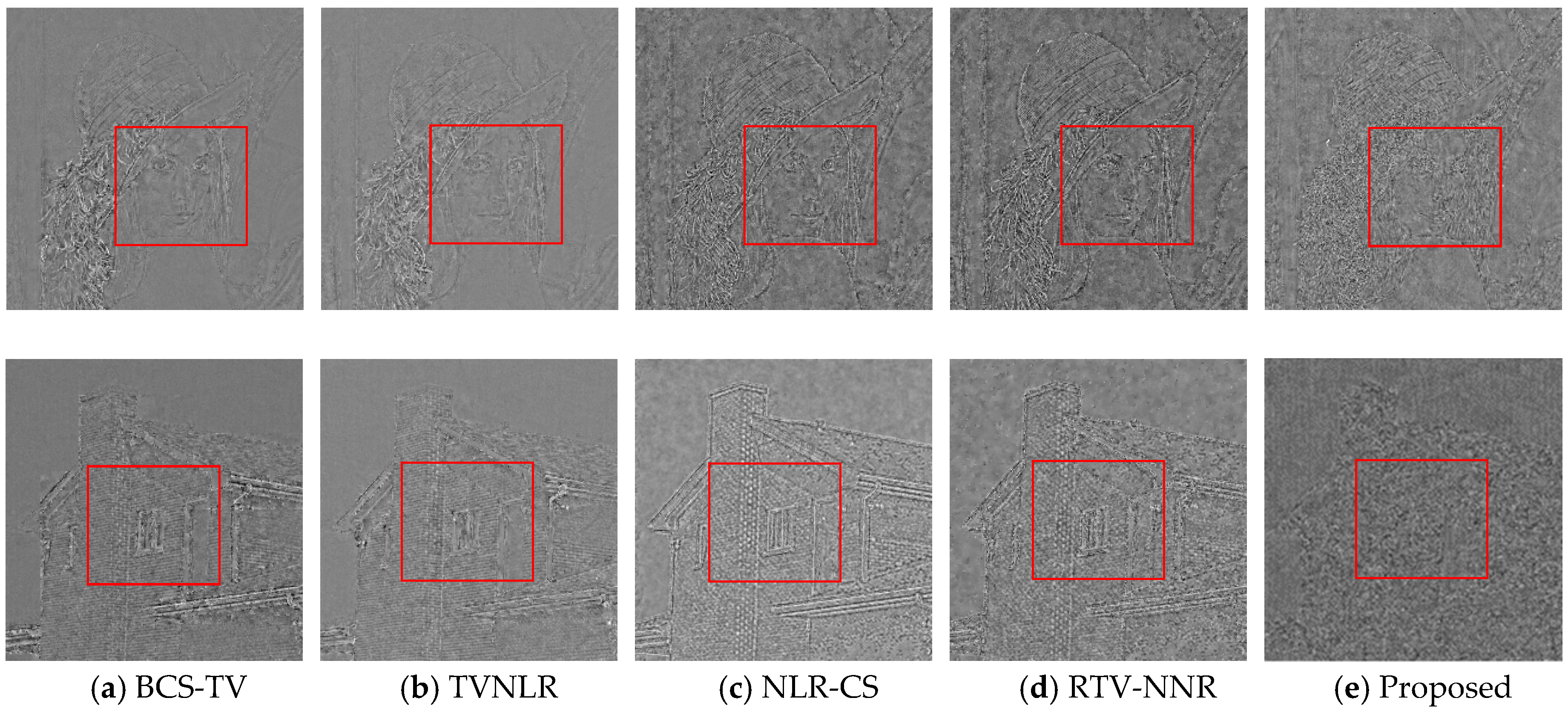
Intuitively, the visual results of the two images are shown in Figure 6 and the residual images (difference between original images and estimated images) are shown in Figure 7. Selecting portions of reconstructed images in red boxes and enlarging them, we compare them at 5% sampling ratios to appear significant differences. The quality of images reconstructed by BCS-TV and TVNLR are much worse than from the other three algorithms. Many block artifacts can be seen in Figure 6a,b. From Figure 7a,b, the smooth regions are preserved well but the texture details are lost a lot, therefore BCS-TV and TVNLR have bad visual effects. Images reconstructed by NLR-CS are better and have better visual effects. But this algorithm suffers from over-smoothed effects owing to the average tendency of different similar patches. Our proposed algorithm has the best visibility compared with other algorithms in Figure 6. This method preserves image texture details and eliminates staircase artifacts by using the fractional-order differential method and nonlocal regularization. We can hardly see the intact contour in residual images in Figure 7e. Experimental results demonstrate that our proposed method enhances high frequency components (image details) significantly.
Moreover, we acquire SSIM for the sampling ratios of 5% in Table 2. Table 2 shows that BCS-TV and TVNLR are much worse than others and the SSIM of the proposed algorithm are better than the other algorithms for every image. Compared with the second-best method RTV-NNR, our proposed algorithm outperforms by up to 0.0114.
To demonstrate that our proposed algorithm is better for enhancing high frequency components, we decompose the original images and reconstructed images into smooth regions and texture details by using Equations (13) and (14). The texture details of reconstructed images are shown in Figure 8.
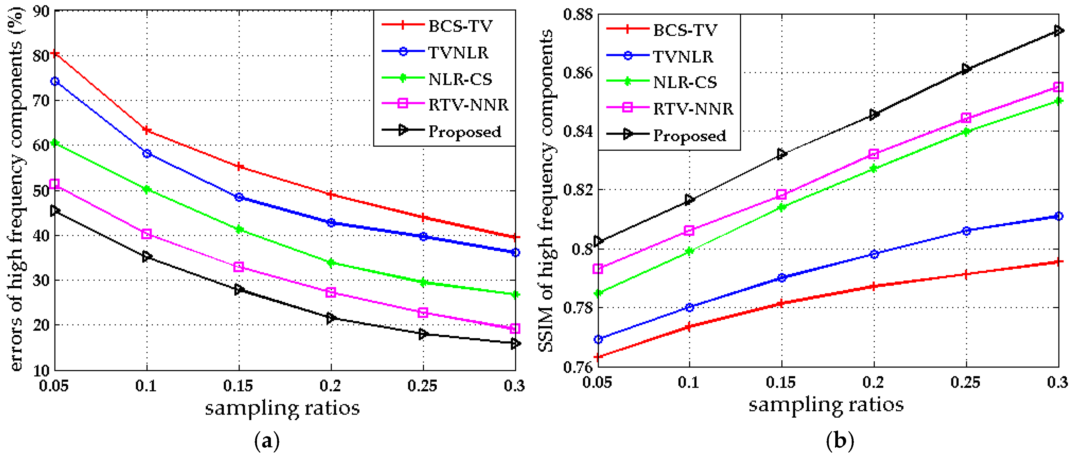
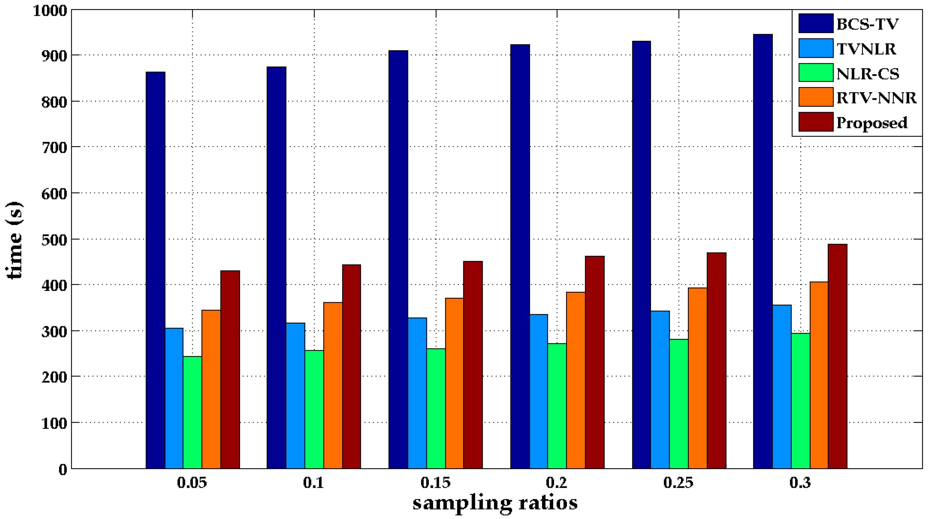
It is clear that our proposed algorithm preserves the most textures in Figure 8 and we can see the complete edge contour. The other four algorithms lost many details, resulting in the terrible visibility in Figure 8. Furthermore, we compare the average relative errors and SSIM of texture details in Figure 9. For every image and sampling ratio, our algorithm has the smallest relative errors and the best SSIM of high frequency components. These results demonstrate that our proposed algorithm enhances the texture details significantly. Compared with other methods, our algorithm lost some low frequency components, but fortunately it has little effect on the visibility of images. We also compare the average reconstruction time at different sampling ratios in Figure 10 and it is shown that our algorithm costs a little more time than TVNLR, NLR-CS and RTV-NNR, but less than BCS-TV, which we will improve in the future.

5. Discussion and Conclusions

We propose a reweighted fractional-order total variation (TV) algorithm with the nonlocal regularization model in order to eliminate staircase artifacts and preserve texture details. We decomposed the images into high and low frequency components and only reweighted the high frequency gradients. The nonlocal regularization model contains prior structural information to suppress staircase artifacts and recover texture details. It is crucial for choosing the appropriate parameters which tends to affect the reconstruction performance and we make trade-offs between all parameters and the reconstruction time. The experiment results demonstrate that the proposed method has the better PSNR and SSIM than the other four methods when the sampling ratio is lower than 25%. The PSNR gains are up to 7.54, 7.15, 3.41 and 1.63 dB from ten images, compared with BCS-TV, TVNLR, NLR-CS and RTV-NNR, respectively. Texture details are preserved, and staircase artifacts are eliminated effectively. Our proposed algorithm enhances the high frequency components at the cost of losing some low frequency components, which has almost no effect for visibility. However, this method has a slightly longer duration than the TVNLR, NLR-CS and RTV-NNR methods. In the further research, we will apply this approach to a single-pixel imaging system for calculating the image of an actual object, owing to its excellent reconstruction quality at low sampling ratios.

Author Contributions

Concept and structure of this paper, H.C.; resources, Y.Q. and H.R.; supervision, L.C.; writing—original draft, H.C.; writing—review and editing, Y.Q., Y.H. and H.Z. All authors have read and agreed to the published version of the manuscript.

Funding

This work was supported by the National Natural Science Foundation of China (NSFC) (61675184 and 61405178); Natural Science Foundation of Zhejiang Province (LY18F010023).

Conflicts of Interest

The authors declare no conflict of interest.

References

  1. Donoho, D.L. Compressed sensing. IEEE Trans. Inf. Theory 2006, 52, 1289–1306. [Google Scholar] [CrossRef]
  2. Candès, E.J.; Wakin, M.B.; Wakin, M.B. An introduction to compressive sampling. IEEE Signal Process. Mag. 2008, 25, 21–30. [Google Scholar] [CrossRef]
  3. Edgar, M.P.; Gibson, G.M.; Bowman, R.W.; Sun, B.; Radwell, N.; Mitchell, K.J.; Welsh, S.; Padgett, M.J. Simultaneous real-time visible and infrared video with single-pixel detectors. Sci. Rep. 2015, 5, 10669. [Google Scholar] [CrossRef] [PubMed]
  4. Ragab, M.; Omer, O.A.; Abdel-Nasser, M. Compressive sensing MRI reconstruction using empirical wavelet transform and grey wolf optimizer. Neural Comput. Appl. 2020, 32, 2705–2724. [Google Scholar] [CrossRef]
  5. Kanno, H.; Mikami, H.; Goda, K. High-speed single-pixel imaging by frequency-time-division multiplexing. Opt. Lett. 2020, 45, 2339–2342. [Google Scholar] [CrossRef]
  6. Candès, E.J.; Tao, T. Near-Optimal signal recovery from random projections: Universal encoding strategies? IEEE Trans. Inf. Theory 2006, 52, 5406–5425. [Google Scholar] [CrossRef] [Green Version]
  7. Edgar, M.P.; Gibson, G.M.; Padgett, M.J. Principles and prospects for single-pixel imaging. Nat. Photon. 2019, 13, 13–20. [Google Scholar] [CrossRef]
  8. Candès, E.; Romberg, J. Sparsity and incoherence in compressive sampling. Inverse Probl. 2007, 23, 969–985. [Google Scholar] [CrossRef] [Green Version]
  9. He, L.; Chen, H.; Carin, L. Tree-structured compressive sensing with variational bayesian analysis. IEEE Signal Process. Lett. 2010, 17, 233–236. [Google Scholar]
  10. He, L.; Carin, L. Exploiting Structure in Wavelet-Based Bayesian Compressive Sensing. IEEE Trans. Signal Process. 2009, 57, 3488–3497. [Google Scholar]
  11. Di Serafino, D.; Landi, G.; Viola, M. ACQUIRE: An inexact iteratively reweighted norm approach for TV-based Poisson image restoration. Appl. Math. Comput. 2020, 364, 124678. [Google Scholar] [CrossRef]
  12. Yang, J.-H.; Zhao, X.-L.; Ma, T.-H. Remote sensing images destriping using unidirectional hybrid total variation and nonconvex low-rank regularization. J. Comput. Appl. Math. 2020, 363, 124–144. [Google Scholar] [CrossRef]
  13. Li, C.; Yin, W.; Jiang, H.; Zhang, Y. An efficient augmented Lagrangian method with applications to total variation minimization. Comput. Optim. Appl. 2013, 56, 507–530. [Google Scholar] [CrossRef] [Green Version]
  14. Zhang, J.; Liu, S.; Xiong, R.; Ma, S.; Zhao, D. Improved total variation based image compressive sensing recovery by nonlocal regularization. IEEE Int. Symp. Circuits Syst. 2013, 2836–2839. [Google Scholar] [CrossRef]
  15. Zhang, M.; Desrosiers, C.; Zhang, C. Effective compressive sensing via reweighted total variation and weighted nuclear norm regularization. IEEE Int. Conf. Acoust. Speech Signal Process. 2017, 1802–1806. [Google Scholar] [CrossRef]
  16. Candes, E.J.; Wakin, M.B.; Boyd, S.P. Enhancing sparsity by reweigh ted l1 minimization. J. Fourier Anal. Appl. 2008, 14, 877–905. [Google Scholar] [CrossRef]
  17. Dong, W.; Shi, G.; Li, X.; Ma, Y.; Huang, F. Compressive Sensing via Nonlocal Low-Rank Regularization. IEEE Trans. Image Process. 2014, 23, 3618–3632. [Google Scholar] [CrossRef]
  18. Gu, S.; Zuo, W.; Xie, Q.; Meng, D.; Feng, X.; Zhang, L. Convolutional Sparse Coding for Image Super-Resolution. In Proceedings of the 2015 IEEE International Conference on Computer Vision, Santiago, Chile, 7–13 December 2015; pp. 1823–1831. [Google Scholar]
  19. Yang, X.; Zhang, J.; Liu, Y.; Zheng, X.; Liu, K. Super-resolution image reconstruction using fractional-order total variation and adaptive regularization parameters. Vis. Comput. 2019, 35, 1755–1768. [Google Scholar] [CrossRef]
  20. Pu, Y.-F.; Zhou, J.-L.; Yuan, X. Fractional differential mask: A fractional differential-based approach for multiscale texture enhancement. IEEE Trans. Image Process. 2010, 19, 491–511. [Google Scholar]
  21. Wang, W.; Li, F.; Ng, M.K. Structural similarity-based nonlocal variational models for image restoration. IEEE Trans. Image Process. 2019, 28, 4260–4272. [Google Scholar] [CrossRef]
  22. Jidesh, P.; Kayyar, S.H. Non-local total variation regularization models for image restoration. Comput. Electr. Eng. 2018, 67, 114–133. [Google Scholar] [CrossRef]
  23. Mun, S.; Fowler, J.E. Block compressed sensing of images using directional transforms. In Proceedings of the IEEE International Conference on Image Processing, Cairo, Egypt, 7–10 November 2009; pp. 3021–3024. [Google Scholar]
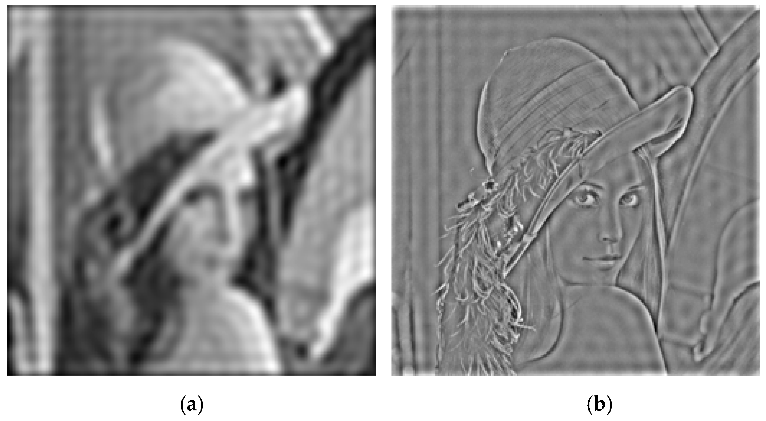
Figure 1. De-high and De-low frequency images of Lena: (a) low frequency components; (b) high frequency components.
Electronics 09 01103 g001
Figure 2. The original images.
Electronics 09 01103 g002
Figure 3. Reconstructed images (Barbara) and the residual images with various fractional order v, the sampling ratios is equal 30%.
Electronics 09 01103 g003aElectronics 09 01103 g003b
Figure 4. PSNR for Barbara at different sampling ratios with different v.
Electronics 09 01103 g004
Figure 5. The PSNR curves of four images: (a) Lena, (b) House, (c) Boats, (d) Chart2.
Electronics 09 01103 g005
Figure 6. Reconstructed images by five methods for a sampling ratio of 5%.
Electronics 09 01103 g006
Figure 7. The residual errors obtained by five methods.
Electronics 09 01103 g007
Figure 8. The texture details of reconstructed images obtained by five methods.
Electronics 09 01103 g008
Figure 9. The average relative errors and SSIM of high frequency components with different ratios: (a) average relative errors of high frequency components, (b) average SSIM of high frequency components.
Electronics 09 01103 g009
Figure 10. Average reconstruction time of five algorithms with different ratios.
Electronics 09 01103 g010
Table 1. Peak signal-to-noise ratios (PSNR) comparisons of five algorithms (unit: dB).
ImageMethodSampling Ratios
0.050.10.150.20.250.3
LenaBCS-TV23.3425.7128.0829.6130.9431.82
TVNLR24.4226.4728.6230.3331.3132.22
NLR-CS26.6828.7030.4632.0233.5834.67
RTV-NNR27.8230.1131.8133.3434.7736.00
Proposed29.6431.3432.7333.9734.9235.85
BarbaraBCS-TV20.1822.7524.6126.1227.5528.95
TVNLR21.2623.0124.7226.6828.3329.69
NLR-CS24.3126.0427.6929.2230.6731.99
RTV-NNR26.0927.8829.5031.1232.7234.15
Proposed27.7229.4230.8632.0133.1834.20
CameramanBCS-TV20.4323.2925.4727.8229.9631.14
TVNLR21.2623.8925.9028.0830.1931.64
NLR-CS24.1226.2928.0529.8731.6033.07
RTV-NNR25.8327.7729.4231.0832.7034.21
Proposed27.3028.9230.4631.7332.7533.84
MonarchBCS-TV19.9422.3424.9226.8028.4630.00
TVNLR20.8323.2725.9827.5829.1631.02
NLR-CS23.9126.2928.1029.7831.3532.81
RTV-NNR25.3627.4629.3131.1933.0434.66
Proposed26.6228.3430.0631.5933.0134.47
ParrotsBCS-TV26.6428.8330.5931.8332.9434.01
TVNLR27.3029.5431.2632.7934.3035.66
NLR-CS29.6631.6433.4635.0336.6338.11
RTV-NNR30.3532.3234.1535.7437.3338.85
Proposed31.1432.9834.5736.0237.4138.63
ClockBCS-TV24.7527.5229.3031.0432.4432.78
TVNLR25.4928.3530.2931.9832.5633.67
NLR-CS27.8029.7631.5533.1734.6835.90
RTV-NNR29.0131.1332.8434.3435.7636.92
Proposed30.4832.2333.8935.2136.3437.10
HouseBCS-TV24.1227.5129.5031.2332.4333.36
TVNLR26.9729.8231.5233.1734.3235.24
NLR-CS28.7730.9132.6834.0335.2636.40
RTV-NNR29.3331.3233.1234.7535.8436.63
Proposed30.6032.2933.7035.1536.2936.94
BoatsBCS-TV22.2624.2926.4427.9828.9830.22
TVNLR22.8824.9527.0828.7229.9031.03
NLR-CS25.0526.9428.7530.2831.6632.84
RTV-NNR26.5228.3329.9931.4232.9634.04
Proposed28.1129.7131.1332.3933.3634.17
Chart1BCS-TV15.9719.3322.4626.8430.7033.43
TVNLR16.0421.4825.6929.7233.8436.82
NLR-CS21.1225.3128.9332.4635.6638.35
RTV-NNR22.7126.5530.0433.3936.3739.07
Proposed23.1927.2030.3333.2536.0438.44
Chart2BCS-TV16.4820.8123.9126.2528.0729.99
TVNLR17.7421.7325.4528.0429.7930.69
NLR-CS20.4224.0827.5330.4132.9535.22
RTV-NNR22.1025.6528.9031.7534.1436.23
Proposed23.6726.7829.9232.4834.5436.39
Table 2. The values of the structural similarity index (SSIM) for the different images (ratio: 0.05).
ImageBCS-TVTVNLRNLR-CSRTV-NNRProposed
Lena0.81220.81780.84920.85020.8616
Barbara0.80830.81270.83940.85690.8671
Cameraman0.79740.80340.82800.83630.8390
Monarch0.76320.76920.78480.79310.7992
Parrots0.85870.86320.87530.88320.8926
Clock0.86130.86800.88140.89470.8982
House0.87030.87750.89370.90610.9082
Boats0.80890.81970.83160.84300.8538
Chart10.62850.63200.65770.67830.6850
Chart20.65930.66270.68040.69220.7008