Article

Improved Dominance Soft Set Based Decision Rules with Pruning for Leukemia Image Classification

1
Department of Information Technology, Sona College of Technology (Autonomous), Salem, Tamil Nadu 636005, India
2
Department of Computer Science, Periyar University, Salem, Tamil Nadu 636 011, India
3
Robotics and Internet-of-Things Lab (RIOTU), Prince Sultan University, Riyadh 11586, Saudi Arabia
4
Faculty of Computers and Artificial Intelligence, Benha University, Benha 13511, Egypt
5
Faculty of Engineering, Cairo University, Giza 12613, Egypt
*
Author to whom correspondence should be addressed.
Electronics 2020, 9(5), 794; https://doi.org/10.3390/electronics9050794
Submission received: 24 February 2020 / Revised: 12 April 2020 / Accepted: 1 May 2020 / Published: 12 May 2020
(This article belongs to the Special Issue Machine Learning Applied to Medical Image Analysis)

Abstract

:
Acute lymphoblastic leukemia is a well-known type of pediatric cancer that affects the blood and bone marrow. If left untreated, it ends in fatal conditions due to its proliferation into the circulation system and other indispensable organs. All over the world, leukemia primarily attacks youngsters and grown-ups. The early diagnosis of leukemia is essential for the recovery of patients, particularly in the case of children. Computational tools for medical image analysis, therefore, have significant use and become the focus of research in medical image processing. The particle swarm optimization algorithm (PSO) is employed to segment the nucleus in the leukemia image. The texture, shape, and color features are extracted from the nucleus. In this article, an improved dominance soft set-based decision rules with pruning (IDSSDRP) algorithm is proposed to predict the blast and non-blast cells of leukemia. This approach proceeds with three distinct phases: (i) improved dominance soft set-based attribute reduction using AND operation in multi-soft set theory, (ii) generation of decision rules using dominance soft set, and (iii) rule pruning. The efficiency of the proposed system is compared with other benchmark classification algorithms. The research outcomes demonstrate that the derived rules efficiently classify cancer and non-cancer cells. Classification metrics are applied along with receiver operating characteristic (ROC) curve analysis to evaluate the efficiency of the proposed framework.

1. Introduction

During the last few decades, digital image analysis has been enriched with significant advancements and new techniques. A large volume of medical image digital data has been captured and recorded by way of regular clinical observation, research, and analysis. In the field of medical image analysis, various kinds of image processing and analysis techniques have been developed and applied to extract clinical data from the captured images. Despite these advancements in science and technology, in oncology studies, medical practitioners experience uncertainties when classifying malignant features. This constraint has prompted many researchers to design frameworks to analyze the image and to diagnose the disease accurately so that better treatment could be given to the patient at the right time. Leukemia is a collective term applied to a group of malignant diseases with significant myeloid or lymphoid impacts. Manual evaluation of the picture of microscopic leukemia is less reliable and time-consuming, making it impossible for the hematologist to correctly interpret the features of the leukemia cells. Recent researchers have used various statistical and image recognition methods to classify leukemia cells. Two broad types of leukemia are recognized, acute and chronic, depending upon the degree of development of the disease. Acute lymphoblastic leukemia (ALL) is the most prevalent group of cancer in adolescents.
The National Cancer Institute of the United States foresees that in the year 2019, there will be around 60,300 new instances of leukemia are identified and out of which 24,370 people will meet fatality [1]. In India, leukemia is found to be the ninth leading cause among youngsters of age under 14 years [2]. In the case of boys, the highest age-adjusted incidence rate (AAIR) and the lowest AAIR are reported as 101.4 and 8.4 in Delhi and Meghalaya, respectively. Concerning girls, the highest AAIR of leukemia is recorded in Delhi as 62.3, and the lowest AAIR is Cachar District, Assam as 6.3 [3]. Early detection and complete remission of leukemia are the most challenging tasks for the Oncologists. Globally, several research institutions are striving towards finding effective treatment of leukemia [4]. The correct and timely diagnosis of leukemia helps a lot in implementing the right treatment to cure leukemia. The present research focuses on the application of rough set theory and an extension of soft set theory for diagnosing ALL from blood microscopic images.
Particle swarm optimization (PSO) is a popular evolutionary computation method introduced by Kennedy and Eberhart in 1995. The inspiration for this concept came from observing the social behavior of bird flocking [5]. It is a powerful population-based optimization technique that has been applied successfully to a wide variety of search and optimization techniques, including some image processing problems such as image segmentation, feature selection, and classification [6,7,8,9,10]. In this paper, we describe an image process by which a leukemia nucleus is segmented in the image applying the PSO algorithm, and subsequently, and we present how relevant representative features are extracted from the segmented nucleus. During this process, different kinds of features, namely, shape, color, and texture features, are extracted. In texture features, grey level co-occurrence matrix (GLCM) is computed for the dimensions 0°, 45°, 90°, and 135°.
In image processing, a large number of features can be extracted, and it leads to the following issues. (1) Complete feature sets decrease the prediction accuracy. (2) They also reduce the processing speed or computational time. This is where feature selection comes into the picture. Feature selection (FS) is the procedure of choosing a common subset of features that is most correlated to the decision classes [11]. Molodtsov [12] designed a kind of soft set theory. It is an innovative mathematical tool to deal with ambiguity and imprecision in the leukemia images and is widely used for medical image processing. Its application in the decision-making process is much contemplated. Maji et al. discussed the application of soft set theory in decision making [13]. Isa et al. proposed an extension of soft set theory involving dominance relation. It is used to deal with uncertainty occurring in the process of multiple criteria-based decision making. In this research, improved dominance soft set-based decision rules are derived to classify the blast and non-blast cell images.

1.1. Research Motivation

Medical imaging has improved the comprehension of the auxiliary and useful design of human life structures and is broadly utilized for the discovery, mediation, and administration of clinical issues. The inspiration for our recent research comes from the potential of dominance soft set theory and its application in the medical field. The overarching of our research is the design of computational algorithms for extracting relevant features from a segmented nucleus and reducing its dimensionality. Our method analyzes digital images of leukemia cells, and the derived rules are utilized to classify the blast and non-blast cells. This approach allows us to interpret the visual information of the cellular elements in a similar way to the one that we use our senses to identify objects. The proposed solution for cell morphology analysis follows a methodology that uses soft computing and data mining techniques. This methodology includes segmentation, feature extraction, feature selection, classification, and diagnosis of acute leukemia. In the existing approach, the decision rules are generated based on the dominance-based soft approximation. To enhance the performance of the proposed approach, AND operation in multi-soft set theory is employed in the dominance-based soft approximation. This leads to computing the dependency of the reduct set and decision rules are generated. The derived rules are then simplified by using a rule pruning algorithm [14] which reduces the classification processing time. From the experimental results, it is deduced that the overall classification accuracy of the proposed IDSSDRP is 98.08%, 97.12%, 99.04%, 97.60%, and 95.67% for GLCM_0, GLCM_45, GLCM_90, GLCM_135, and shape and colour datasets respectively. The ROC curve of the IDSSDRP algorithm appears in the top left border of the ROC graph which becomes more significant. This means that the proposed approach correctly differentiates the blast and non-blast cells when compared to the existing traditional approaches.

1.2. Research Contribution

The research contributions of this work are enumerated below:
  • A new algorithm is applied to segment the leukemia nucleus based on Particle Swarm Optimization (PSO), which is a popular search optimization algorithm.
  • The Haralick texture-based GLCM is employed to extract features in four directions, and shape and color based features from the segmented image.
  • Improved dominance soft set-based decision rules with pruning algorithm (IDSSDRP) is applied to classify the leukemia cancerous image. This is carried out in three phases:
    • In the first phase, an improved dominance soft set-based reduction technique using AND operation in multi-soft set is applied to find the reduct set.
    • In the second phase, the dominance soft set-based approach is applied to generate decision rules. Receiver operating characteristic (ROC) curve analysis is used to evaluate the efficiency of the proposed decision rules.
    • In the third phase, the rule pruning method is employed to simplify the rules to minimize the processing time for predicting the diseases (tumor image).
  • Different classification algorithms are evaluated using appropriate classification measures.
The rest of the paper is organized as follows. Section 2 presents the literature survey of related works on leukemia image analysis and soft set theory. Section 3 explains the methods and materials. Section 4 discusses the proposed method of decision rules making and pruning algorithm with numerical example. Detailed empirical results of the research paper are discussed in Section 5. Finally, Section 6 presents the conclusion and indicates the scope of further research.

2. Related Work

Applications of soft set theory and its extensions are discussed as follows: In [15], dominance-based rough fuzzy approximations (DFRSA) of an upward or downward cumulated fuzzy set were explained. Attributes reduction was performed using rough set theory based on the discernibility matrix and the heuristic strategy. Fuzzy dominance relation was then used to extract the decision rules. A case study in bankruptcy risk analysis was employed to verify the performance of the DFRSA method. In [16], the authors established soft-dominance relation based on soft set theory in the area of multi-criteria decision analysis.
Many researchers have worked in the field of soft set theory and its extension. In [17], the researchers discussed how various hybrid soft set models could be utilized in the field of decision making. Karaaslan [18] introduced two possible neutrosophic soft sets, namely AND-product and OR-product, to apply in decision-making problems. The arithmetical illustration displays the applications of the neutrosophic soft decision-making method, also called the PNS-decision making method. In [19], the bijective soft set was utilized to generate decision rules. Various medical datasets were analyzed, and the empirical results showed that the bijective soft set-based decision rules effectively classified the diseases. Z-soft fuzzy rough sets-based decision making was proposed by Zhan Jianming et al. [20]. In this approach, some other types of soft set models were also investigated. The mathematical results showed that the proposed method reduced the computational time when compared to other hybrid soft set models. In [21], the association between rough sets, soft sets, and hemirings was examined. The concept of soft, rough hemirings was applied to solve multi-criteria group decision-making problems. Some theoretical concepts of C-soft sets, CC-soft sets, and BC-soft sets lower and upper MSR-hemirings (k-ideals and h-ideals) were also discussed.
The study of blood microscopic images is the most challenging task for automatic detection of tumors from blood microscopic images. Currently, many researchers analyze the leukemia images to detect the blast cells using various machine learning and soft computing techniques. In [22], the author(s) developed an automated technique for white blood cell recognition and categorization. This approach is necessary to analyze each cell component in detail. Different features, namely shape-based, color-based, and texture-based features, are extracted using a new approach for background pixel removal. This process works very well and allows for the early diagnosis of suspicious cells. In [23], the researchers employed an ensemble classifier to predict the ALL in blood microscopic images. It is observed that an ensemble of classifiers leads to higher accuracy in comparison with the existing classifiers, namely Naive Byes, KNN, MLP, RBNF, and SVM.
In [24], the authors described a histogram-based soft covering rough K-means clustering (HSCRKM) algorithm for leukemia nucleus image segmentation. This approach incorporates the benefits of a soft covering rough set and rough k-means clustering. The histogram method is utilized to find the number of clusters to avoid random initialization. Machine learning algorithms were applied to categorize the healthy and leukemia cells. The proposed approach is compared with an existing clustering algorithm, and the efficiency is evaluated based on the prediction metrics. The results indicate that the HSCRKM method efficiently segments the nucleus, and it is also inferred that logistic regression and neural networks perform better than other classification algorithms.
In [25], the authors have developed a computer-aided system to detect acute lymphoblastic leukemia cells. In this approach, discrete orthonormal S-transform has been utilized to extract texture features and linear discriminant analysis is employed to reduce the dimension of the feature set. Adaboost algorithm with random forest (ADBRF) classification algorithm has been proposed to distinguish the blast and non-blast cells. The simulation results based on the five runs of K-fold cross-validation indicate that the proposed method yields superior accuracy as compared to existing schemes.
In [26], the author(s) have designed a graphical user interface (GUI) technique to differentiate acute lymphoblastic leukemia nucleus from healthy lymphocytes in an image. In this approach, three kinds of hybrid metaheuristic algorithm, namely supervised tolerance rough set PSO based quick reduct (STRSPSO-QR), supervised tolerance rough set PSO based relative reduct (STRSPSO-RR), and supervised tolerance rough set firefly based quick reduct (STRSFF-QR), have been applied to eliminate the redundant features. The selected features were then fed into the classification process and the generated rules were optimized using the Jaya algorithm. The experimental results showed that, after improving the Jaya algorithm, the accuracy of the classification was improved.
In [27], the authors have presented an automatic leukocyte cell segmentation process using a machine learning approach and image processing technique. The features were extracted using four-moment statistical features and artificial neural networks (ANNs). It was found that the proposed method for blasts cell segmentation provides better accuracy under different conditions.
In [28], the authors developed a decision support system for Acute Leukaemia classification based on digital microscopic images. In this approach, K-means clustering is used to segment the leukemia cells and the features are extracted. The developed system was classified as leukemia cells according to their morphological features. A total of 757 images were collected from two datasets labeled with three different categories, such as blast, myelocyte, and segmented cells. The experimental results show that the proposed approach achieved promising results.

3. Methods and Materials

The system architecture of tumor detection in acute lymphoblastic leukemia using improve dominance soft set-based decision rule generation with pruning is presented in Figure 1. This architecture contains several processing steps such as input image acquisition, preprocessing, nucleus segmentation, feature extraction, decision rules generation with pruning, and prediction.

3.1. Input Image

The Acute Lymphoblastic Leukemia Image Database, i.e., ALL-IDB2 openly available dataset, was used for this experiment. These data belong to Fabio Scotti Department of Informatics, University of Milan, Italy and were downloaded from the webpage www.dti.unimi.it/fscotti/all/ [29,30,31,32]. It is a collection of normal and blast cell images showing a cropped area of interest. In this dataset, all the image files are named with the symbolization ImXXX_Y.jpg where XXX is a progressive 3-digit integer, and Y is a Boolean digit. The healthy individual, i.e., non-blast cell, is indicated as 0, and blast cell is indicated as 1. In this data set, which is used for experimental analysis, there are 368 images, of which 175 are benign and 193 are malignant.

3.2. Preprocessing

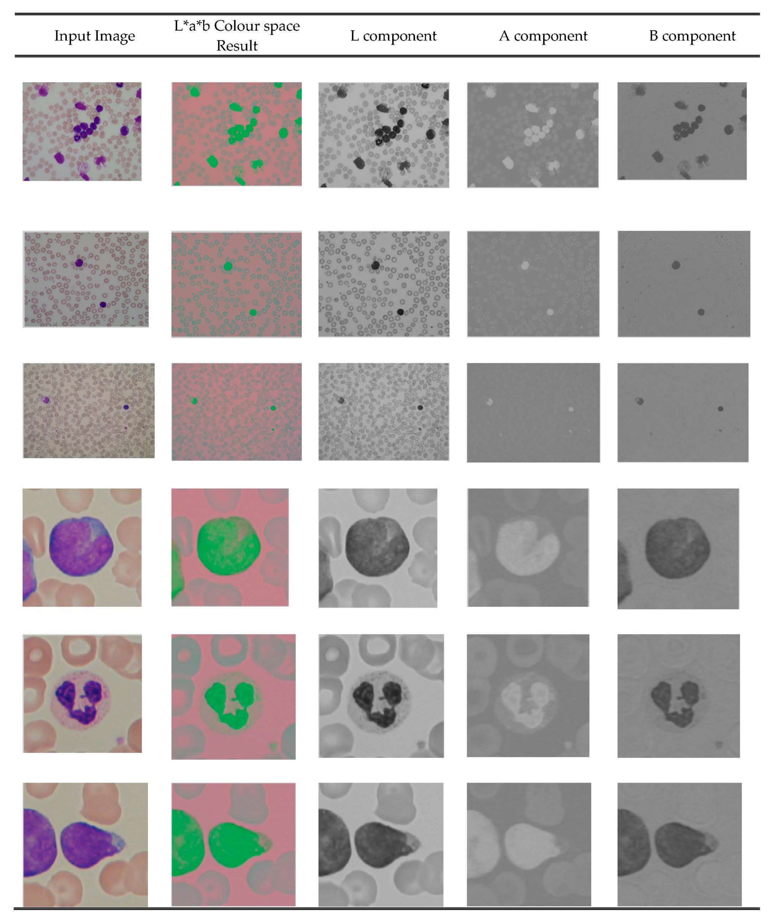
The digital microscope images are RGB color images. The entire ALL Images are generated from digital microscopes and usually in RGB color space, which is difficult to segment. Therefore, the RGB image is converted into a LAB color image. The L*a*b* space consists of a luminosity layer L* and chromaticity layers a* and b*. Here, the color information is represented in two components, i.e., a* and b*. Due to the low color dimension, L*a*b* color space is mostly employed in color-based clustering [33,34]. The sample outputs of LAB color conversion are shown in Figure 2.

3.3. Segmentation

Segmentation is a process used to simplify the representation of an image into a more meaningful image. It facilitates the analysis of images [35]. Segmentation is an important phase in many image processing tasks such as medical image analysis, object identification, tumour detection, satellite imagery, etc. A great variety of segmentation methods has been proposed in the past decades. In this research, the particle swarm optimization (PSO) algorithm, which is a widely used segmentation method, was applied to segment the leukemia nucleus [5].
PSO is initialized with a population of particles. Each image is treated as a particle in an S-dimensional space. The ith particle is represented as X i =   x i 1 , x i 2 , . ,   x iS . The best previous position p best of any particle is   P i =   p i 1 , p i 2 , . ,   p iS . The index of the global best particle is represented by g best . The velocity for each particle is   V i =   v i 1 , v i 2 , . ,   v iS . In each iteration update the particle velocity and positions using the Equations (1) and (2). The pseudo code for PSO algorithm-based segmentation is presented in Algorithm 1.
v id = w × v id + c 1 × rand ( ) × p id x id + c 2 × rand ( ) × p gd x id
x id = x id + v id
Algorithm 1 Pseudo Code for PSO algorithm
I n p u t :   Each   image   is   considered   as   a   particle
O u t p u t :   Segmented   image
For   each   particle
Initialize particle
End
Do
For   each   particle
Calculate   Data   fitness   value
If   the   fitness _ value   is   better   than   pBest
Set   pBest   =   currentfitnessvalue
If   pBest   is   better   than   gBest
Set   gBest   =   pBest
End  
For   each   particle
Calculate   particle _ Velocity
Use   gBest   and   Velocity   to   update   the   particle
End
While maximum   iterations   or   minimum   error   criteria   is   met
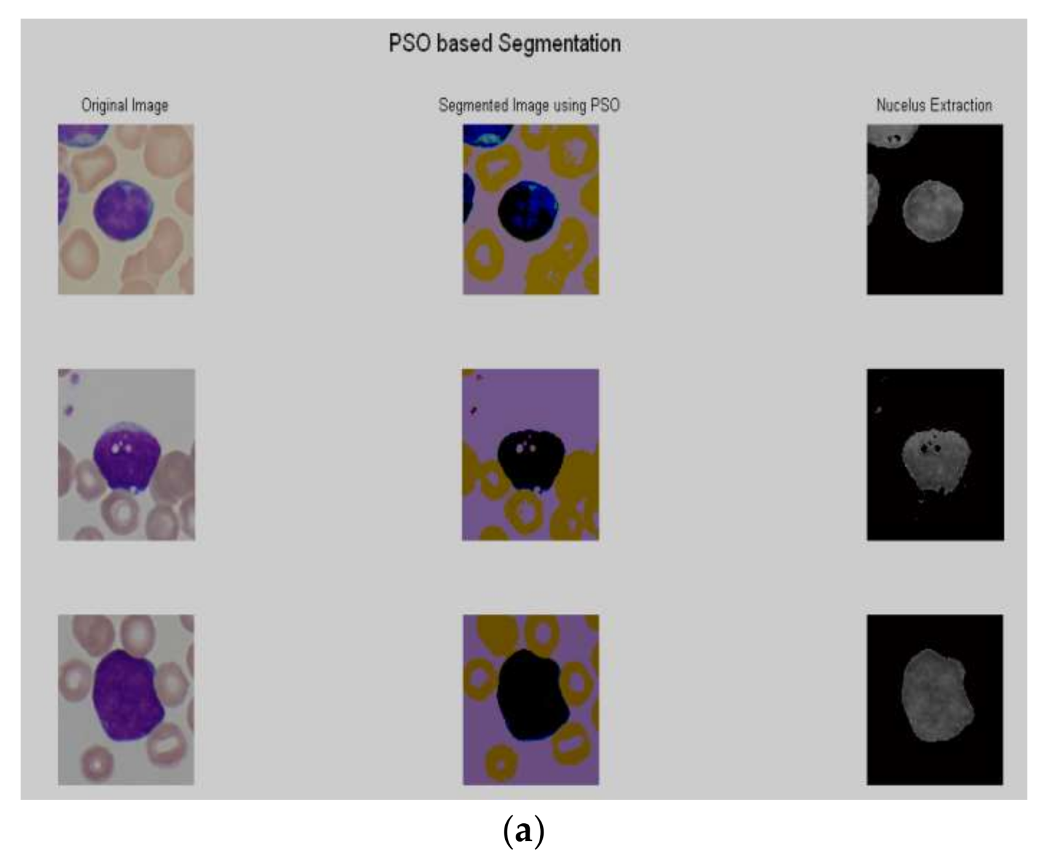
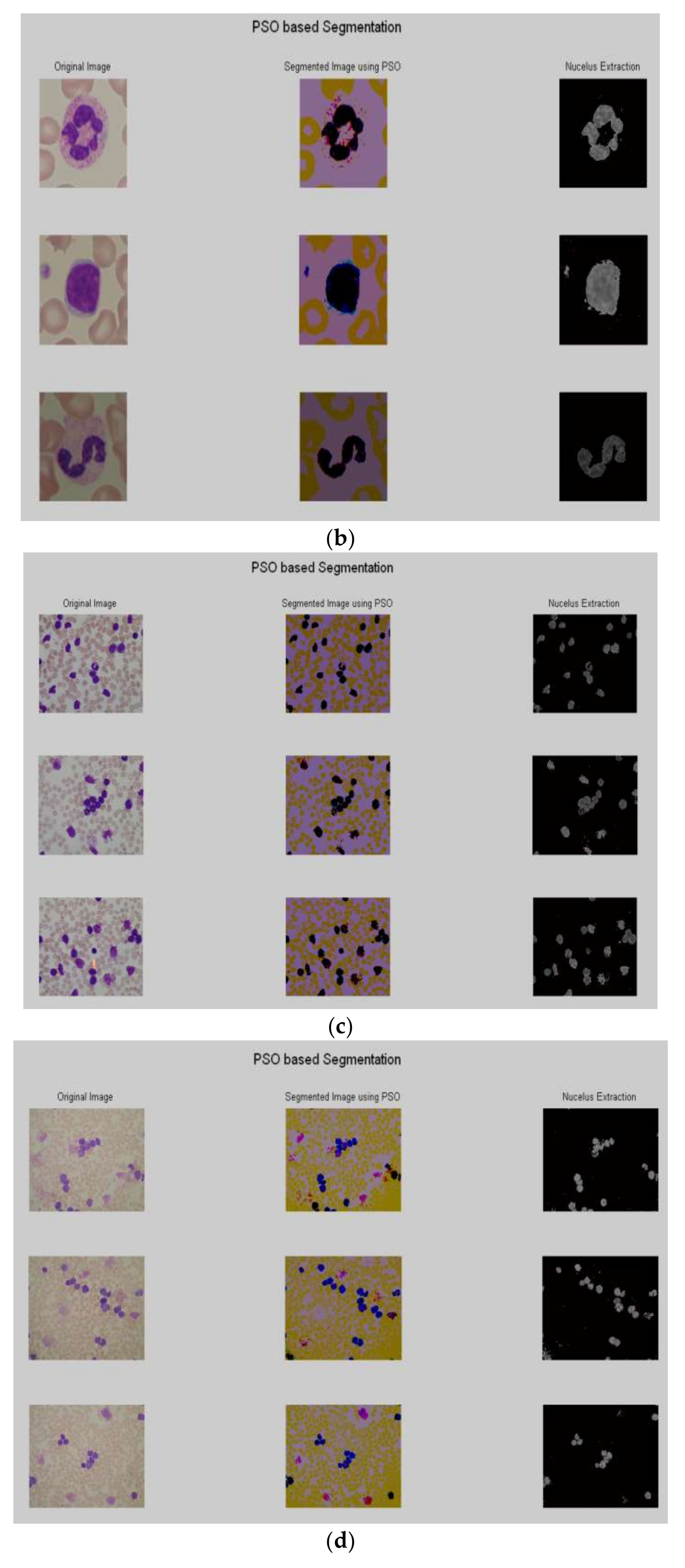
After the preprocessing, PSO based segmentation algorithm was utilized to segment the nucleus. The results of some sample images are shown in Figure 3a–d.

3.4. Feature Extraction

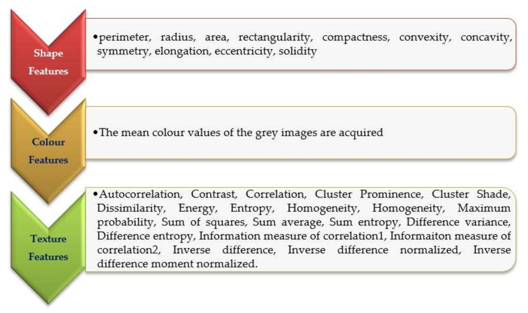
In medical image processing, the process of detection and description of global or local properties of objects present in images is called feature extraction. In the present research, different categories of features were extracted, namely shape-based, color-based, and texture-based features [36,37,38,39]. The leukemia image consists of a massive nucleus of irregular shape and size. The shape is a fundamental feature that describes the physical characteristics of an image. It can be corrupted by noise, random distortion, and obstruction. This leads to image recognition in a more complex process. Colour-based features represent the colour components of an image. Leukemia images are in RGB colour format so that it is a discriminative feature of blood and bone marrow cells [11]. The texture feature describes the organization of the basic elements of an image. Hence, it is not desirable to distinguish the images based on colour-based features alone. Many methods are available to describe the texture features and one of the commonly used measures is the gray-level co-occurrence matrix (GLCM). In this research, GLCM was computed for dimensions 0°, 45°, 90° and 135°. In texture-based features, gray level co-occurrence matrix (GLCM) was computed for the dimensions 00, 450, 900, and 1350. For each segmented image, a total of 110 features were extracted, which consisted of 11 shaped-based features, 88 texture-based features (i.e., each dimension 22 features), and 11 color-based features [40,41,42]. A detailed delineation of the extracted features is presented in Figure 4.

3.5. Dominance Based Soft Set Theory

Dominance-based soft set approach (DSSA) is an extension of soft set theory which is utilized for decision-making analysis [16]. The lower approximation, upper approximation and boundaries of Cl t and Cl t are defined as follows t = 1 , , n
P _ Cl t = x U : D p x Cl t
P ¯ Cl t = x U : D p + x Cl t
P _ Cl t = x U : D p x Cl t
P ¯ Cl t = x U : D p + x Cl t
Bn p Cl t = P ¯ Cl t P _ Cl t
The quality of approximation of the classification by a set of soft set can be defined as [16]:
γ P Cl = U t T Bn P Cl t t T Bn P Cl t U
where γ P Cl   is a degree of consistency of the objects from U , P is the set of criterion soft set, and Cl   is considered as classification. Every minimal subset P C such that γ P Cl = γ C Cl is called a reduct set of Cl   RED Cl .

3.6. Dominance Soft Set Based Decision Rules

Definition 1:
D decision rules
If f x , q 1 r q 1 and f x , q 2 r q 2 and …. f x , qp r qp then x Cl t , where P = q 1 ,   q 2 ,   ,   qp C , r q 1 , r q 2 , . , r qp V q 1 × V q 2 × × V qp and t T . These rules are reinforced by entities from the P soft lower approximation of the upward unions of classes Cl t [16].
Definition 2:
D decision rules
If f x , q 1 r q 1 and f x , q 2 r q 2 and …. f x , qp r qp then x Cl t , where P = q 1 ,   q 2 ,   ,   qp C , r q 1 , r q 2 , . , r qp V q 1 × V q 2 × × V qp and t T . These rules are reinforced by entities from the P soft lower approximation of the downward unions of classes Cl t [16].

4. The Proposed Method: Improved Dominance Soft Set Based Decision Rules with Rule Pruning (IDSSDRP)

In this research, the improved dominance soft set-based decision rules with rule pruning algorithm are proposed to make decision rules to efficiently classify the acute lymphoblastic leukemia images. The proposed system contains three different phases, namely, improved dominance soft set-based attribute reduction (IDSSA) using AND operation in soft set theory, decision rules (DR) making, and rule pruning (PR). In phase 1, improved dominance soft set-based attribute reduction algorithm presented in Algorithm 2 was utilized to select the critical feature which is related to the decision class. The selected features were fed into phase 2 and generated the decision rules based on the Psoft lower, upper, and boundary region values. Finally, in phase 3, the rule pruning algorithm was used to simplify the rules, which reduce the processing time. The detailed description of each phase is defined as follows:
Algorithm 2 Improved dominance soft set-based attributes reduction using AND operation
Phase 1: (Improved Dominance Soft Set based Attributes Reduction using AND operation)
IDSSA C , D
C ,   the   set   of   all   conditional   attributes
D ,   the   decision   attribute
A ,   Attributes   in   multivalued   information   system
1   S    
2   do
3   Construct the Multi-valued information Table (F, S)   C = F ,   S   where S A
U = F , a 1 × a 2 × a 3 × a i   i = no . of   attributes   in   C
4   T   S
5   P C
6   Calculate   Dependency , γ P Cl   using   Equation   9
7   Find   Max γ P C
8     if   γ S P C γ C C
9       T   S P
10       S   T
11   until   γ P Cl =   γ C Cl
12   return   S
In phase 1, the prominent features based on the improved dominance soft set-based attribute reduction using AND operations in multi-soft set are reduced. The conditional features are denoted as c 1 ,   c 2 ,   c 3 .   c n and the decision feature is denoted as D. The IDSSA algorithm begins with an empty set. Then, multi-valued information table (F, S) is constructed [43]. For each conditional feature, P soft   boundaries of Cl t and Cl t   are computed. The dependency value for each feature is calculated using AND operations [44] and the maximum dependency value is obtained. If the conditional feature dependency value γ P Cl is greater than or equal to the dependency value of decision feature, then the reduced feature set S where   P C is retained. Otherwise, a combination of the minimal feature set is taken and the dependency value is calculated. This process is continued until the stopping condition is met.
In phase 2, the decision rule based on the dominance relations is generated as described in Algorithm 3. Here, U is the universal set of features and S = S 1 ,   S 2 ,   S 3 ,   .   S n   is the selected attributes or features. For each selected attribute, the lower approximation of upward and downward unions for the classes of Cl t and Cl t   are computed. The decision rules are derived from the P soft   approximation based on definitions 1 and 2.
Algorithm 3 Decision Rules Generation
Phase 2: (Decision Rules—DR Generation)
DR U , S
U ,   Universal   set
S ,   Selected   attributes
1 Compute   lower   for   the   selected   attributes   S   for   both   the   classes   based   on   Equations   ( 3 )   and   ( 4 ) .  
f U , S Cl 1   P   _ Cl 1
f U , S Cl 2   P   _ Cl 2
2 D decision   rules   derived   from   the   P soft   lower   approximation   of   the   upward   unions   of   classes   Cl 1
3 D decision   rules   derived   from   P soft   lower   approximation   of   the   downward   unions   of   classes   Cl 2
In phase 3, the derived rules are pruned based on the rule pruning method as described in Algorithm 4. Initially, the algorithm begins with an empty set and each rule   R i is assigned to R u . The conditional feature in R u   is eliminated one by one. In each step, it is verified that if the rule R u is inconsistent with any other rules in R i ,   then dropped conditional feature is restored. The resulting rules are stored in   P r . Before the rule R u is added to P r , it is verified for rule redundancy. If rule R u is logically included in any rule in P r , i.e., R u P r then R u is discarded. This process is continued until the last rule is verified. Finally, the pruned rules are accumulated in P r .
Algorithm 4 Decision Rule Pruning
Phase 3: (Rule Pruning—RP)
RP Derived Rules
R ,   Set   of   derived   rules
P r ,   Pruned   rules
1   P r  
2   m =   no .   of   rules   in   R
3   For   i = 1   to   m 1
  R u =   R i
n = R u
4       for   j = 1   to   n 1
Eliminate   the   j th   conditional   feature   C j in   rule   R u
if   R i   inconsistent   with   any   rule   R m   then
Return   the   dropped   feature   C j
end   if
end   for
5       if   R u P r   then
Eliminate   rule   R u
else
  P r   R u P r
end   if
End   for
6   Return   P r

4.1. Case Study

4.1.1. Phase-1 (Attribute Reduction)

The sample dataset of job application acceptance is presented in Table 1. Let a 1 ,   a 2 ,   a 3 ,   a 4   be denoted as the condition attributes and d be denoted as decision attribute.
Reconstruct Table 1 into multi-value information table with respect to each criterion of soft set as presented in Table 2.
F , A = F , a 1 = MBA = 1 , 2 , 7 ,   M . Sc = 3 , 8 ,   MCA = 4 , 5 , 6 F , a 2 = Medium = 1 , 5 ,   Low = 2 , 3 , 8 ,   High = 4 , 6 , 7 F , a 3 = Known = 1 , 2 , 3 , 4 , 5 , 6 ,   Unknown = 7 , 8 F , a 4 = Excellent = 1 , 6 , 8 ,   Normal = 2 , 4 , 5 ,   Good = 3 , 7 F , d = Accept = 1 , 4 , 6 , 7 ,   Reject = 2 , 3 , 5 , 8 U F , a1 AND F , a2 AND F , a3 AND F , a4 = F , a 1 , a 2 , a 3 , a 4 γ d Cl = 1 ;
Compute the P soft   lower approximation and the P soft   upper approximation and the P soft   boundaries of
Cl 1 and   Cl 2 . For the attribute a2,
P _ Cl 1 = 4 , 6 , 7 , P ¯ Cl 1 = 1 , 4 , 5 , 6 , 7 ,   Bn p Cl 1 = 1 , 5 P _ Cl 2 = 2 , 3 , 8 , P ¯ Cl 2 = 1 , 2 , 3 , 5 , 8 , ,   Bn p Cl 2 = 1 , 5
Similarly, the approximation values for all the remaining attributes are computed. Compute dependency value of each attribute as:
  γ a 1 Cl = 0.25 ;   γ a 2 Cl = 1 ;   γ a 3 Cl = 1 ;   γ a 4 Cl = 1 ;
Find the maximum dependency and the condition   γ a 2 Cl   γ d Cl is checked.
Take the combination of attribute a 2 using AND operations in multi-soft set,
F , a 1 × a 2 , F , a 2 × a 3 ,   F , a 2 × a 4   γ a 1 , a 2 Cl = 1 ;   γ a 1 , a 2 Cl = =   γ d Cl RED Cl = a 1 , a 2

4.1.2. Phase-2 (Decision Rules Generation)

The decision rules are derived from RED Cl = a 1 , a 2 .
Compute the P soft   lower approximation   Cl 1 and Cl 2 for the attributes, a 1   and   a 2 .
P _ Cl 1 = 1 , 4 , 6 , 7 P _ Cl 2 = 2 , 3 , 5 , 8
D decision rules are derived from the P soft   lower approximation of the upward unions of classes Cl 1 .
  • Rule 1: if   f c , a 1 MBA   and   f c , a 2 High   then   c Cl 1
  • Rule 2: if   f c , a 1 MBA   and   f c , a 2 Medium   then   c Cl 1
  • Rule 3: if   f c , a 1 MCA   and   f c , a 2 High   then   c Cl 1
  D   decision rules are derived from the P soft –lower approximation of the downward unions of classes   Cl 2 .
  • Rule 4: if   f c , a 1 MBA   and   f c , a 2 Low   then   c Cl 2
  • Rule 5: if   f c , a 1 M . Sc   and   f c , a 2 Low   then   c Cl 2
  • Rule 6: if   f c , a 1 MCA   and   f c , a 2 Medium   then   c Cl 2

4.1.3. Phase-3 (Decision Rule Pruning)

P_Rule = {}
The derived decision rules are {R1, R2, R3… R6} incorporated one by one in D_Rules.
Applying Algorithm 4, each rule is checked for decision consistency with other rules. All the rules are processed and the pruned rules P_Rule are given as follows:
  • Rule 1: if   f c , a 1 MBA   then   c Cl 1
  • Rule 2: if   f c , a 2 High   then   c Cl 1
  • Rule 3: if   f c , a 2 Low   then   c Cl 2
The rule pruning method eliminates a total of three rules one for upward unions of classes and two for downward unions of classes.

5. Results and Discussions

5.1. Performance Analysis of Attribute Reduction Algorithm

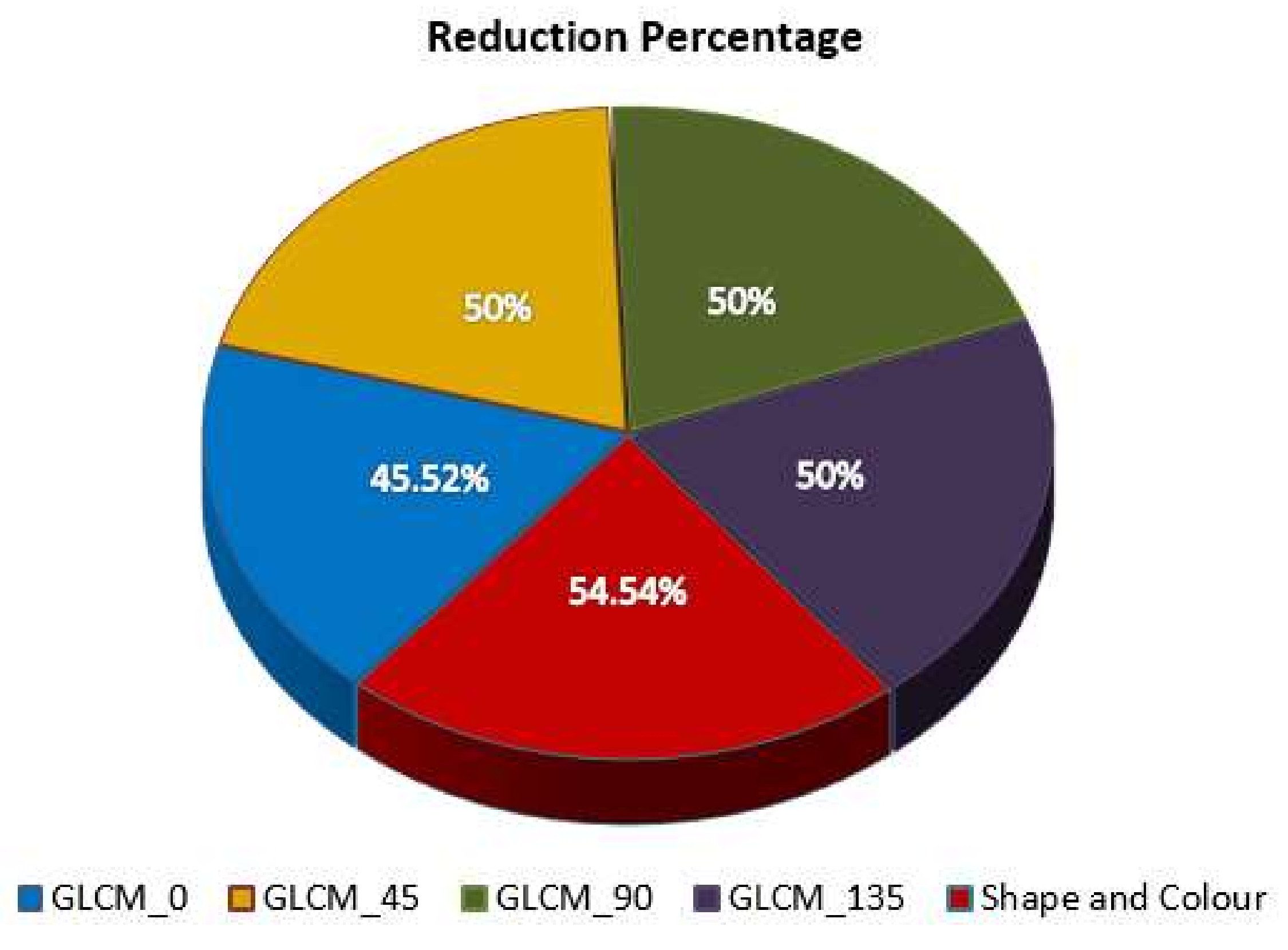
In this research, improved dominance soft set-based attribute reduction (IDSSA) using AND operation in multi-soft set theory was employed to choose the most relevant features. Five different feature datasets, i.e., GLCM_0, GLCM_45, GLCM_90, GLCM_135, and shape-based features were considered. Each feature set contained twenty-two features. On average, the performance of the IDSSA algorithm decreases 50 percent of the features. A detailed description of datasets and the number of features extracted and selected are presented in Table 3.
The reduction percentage for each dataset is presented in a pie chart (Figure 5). From this chart, it can be noted that the modified dominance soft set-based feature selection algorithm eliminates almost 50% of features in all the datasets. With respect to GLCM_0, it is believed that the reduction percentage (45%) is the minimum reduction percentage when compared to all other datasets.

5.2. Evaluation of Proposed IDSSDRP Algorithm

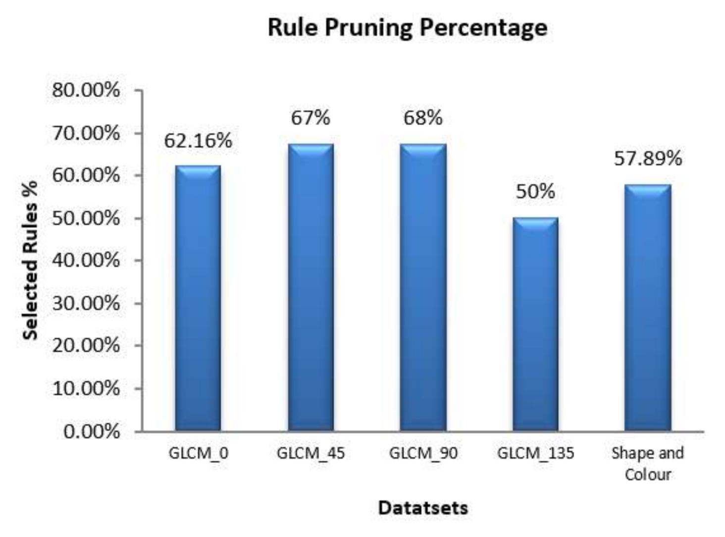
The selected features are then fed into the dominance soft set-based decision rule algorithm. In this algorithm, the lower p-soft and the boundary p-soft approximations are taken as desired rules. In this experiment, five different datasets namely, GLCM-00, GLCM-450, GLCM-900, GLCM-1350, and shape-colour were used to generate the decision rules. For each dataset, 80% of samples were subjected to training and the remaining 20% of samples are used for testing. The decision rule generation algorithm was employed to generate the required rules to predict the tumor image. Finally, the rule pruning algorithm was applied to simplify the obtained rules. The efficiency of the proposed rule pruning algorithm is given in Figure 6.
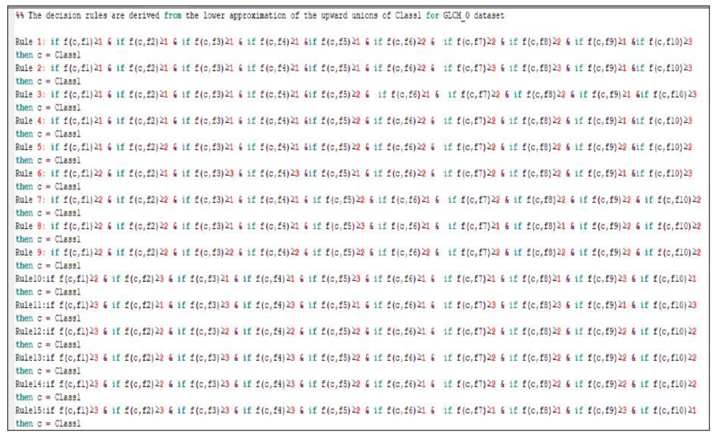
The decision rules are derived from the Psoft lower approximation of the upward and downward unions of class 1 and class 2 for the GLCM_0 dataset as shown in Appendix A. The pruned rules after applying the proposed rule pruning algorithm for the GLCM_0 dataset are shown in Appendix B. The number of rules generated for class 1 is three and that of class 2 is one.
Prediction algorithms that learn from the training set give rise to a more accurate system. This system is utilized to predict new objects. In machine learning, the classifier is evaluated by a confusion matrix. A confusion matrix shows the number of correct and incorrect predictions made by the classification model compared to the actual outcomes (target value) in the data. Table 4 shows the values of entries in the confusion matrix for various classifiers.
The four performance measures have the advantage of being independent of class costs and conceived probabilities. A classifier aims to minimize false positive and negative rates, or conversely to maximize true negative and positive rates. The performance of the proposed algorithm i.e., improved dominance soft set-based decision rule generation with pruning algorithm is compared with other well-known classification algorithms namely, decision tree [45], J48 [46], JRip [47], LMT [48] and random forest [49]. Various classification assessment metrics are used to evaluate the performance of the proposed IDSSDRP algorithm. The detailed interpretation for each metric is presented in Table 5 [50,51,52,53,54,55,56].
Table 6 shows the classification results of the GLCM-0 dataset. Various classification metrics are employed for each classifier with the proposed algorithm. It is noted that the proposed IDSSDRP algorithm performs well when compared to existing classification algorithms.
The error and the balance error rates are very small for the proposed algorithm which indicates that the algorithm classifies the blast and non-blast cell ALL images more accurately.
Table 7 shows the performance of the decision-making algorithms for the GLCM-45 dataset. The proposed IDSSDRP algorithm achieves 97% of overall accuracy and the error rate is 3%. For Youden’s index, the proposed decision-making algorithm achieves the highest score, i.e., 2.5 times better than the average score of existing algorithms.
The efficiency of the proposed algorithm with respect to the GLCM_90 dataset is presented in Table 8. The experimental results for all the five feature extracted datasets are analyzed and it is believed that concerning the GLCM_90 dataset, the highest overall classification accuracy, i.e., 99%, is achieved. The error rate is 0.01, i.e., 1%. It is also noted that the entire classification algorithms have produced prediction accuracy above 80%.
The empirical results of the IDSSDRP algorithm and existing classification algorithms for the dataset GLCM_135 appear in Table 9. It is noted that the classifiers’ decision tree and J48 produced equal values for all the metrics. Furthermore, proposed decision rules almost correctly classified the blast and non-blast ALL images.
Table 10 shows the experimental results of different classification approaches for shape and colour dataset. From the interpretation of results, it is believed that the proposed algorithm achieved 95% of prediction accuracy, which is the minimum accuracy value when compared to the results of other algorithms.
Figure 7 exhibits the performance of decision tree, J48, JRip, random forest, and the proposed DSSRMP for each dataset based on prediction accuracy. It is found that the proposed algorithm gives higher prediction accuracy value. With respect to the GLCM_90 dataset, the highest predication accuracy value, i.e., 99% is achieved. On the contrary, the lowest prediction accuracy value, i.e., 77% is produced by the random forest (RF) classifier concerning the GLCM_135 dataset. It is pointed out that the classifier’s decision trees and J48 achieved a prediction accuracy of about 80%.
The error rate is calculated as the number of all incorrect predictions divided by the total number of inputs. The best error rate is 0.0, however, the worst is 1.0. Figure 8 shows the classification error rate values for various classifiers and the proposed decision-making algorithm with respect to all feature extracted datasets. The proposed IDSSDRP algorithm gives the best error rate values, i.e., less than 0.05. In this graph, it is also noted that the random forest algorithm gives rise to an error rate of 0.23 (relatively higher value) with reference to the GLCM_135 dataset.
Figure 9 illustrates the performance of the proposed and existing algorithms with respect to each dataset, in terms of precision, recall, and F1-measure. Precision, recall, and F1-measure to analyze the performance of the classification algorithms. Precision is defined by how many selected items are relevant whereas recall is defined by how many relevant items are selected. The harmonic means of these two metrics are denoted as F1-measure. From Figure 9, it is observed that the proposed algorithm is compatible and works very well in producing the highest precision, recall, and F1 measure value for the feature extracted datasets.
Table 11 compares the various classification approaches with our proposed IDSSDRP in terms of accuracy, sensitivity, and specificity. In the existing approach [23], SVM classifier gives 91.43% of accuracy, 73.13% of sensitivity, and 98.7% of specificity. From the experimental results, it is revealed that the classification accuracy of the proposed IDSSDRP is 98.08%, 97.12%, 99.04%, 97.60%, and 95.67% for GLCM_0, GLCM_45, GLCM_90, GLCM_135, and shape and colour datasets respectively. It is also noted that, the proposed approach gives more accuracy than SVM classifier.

5.3. Graphical Performance Assessment for IDSSDRP

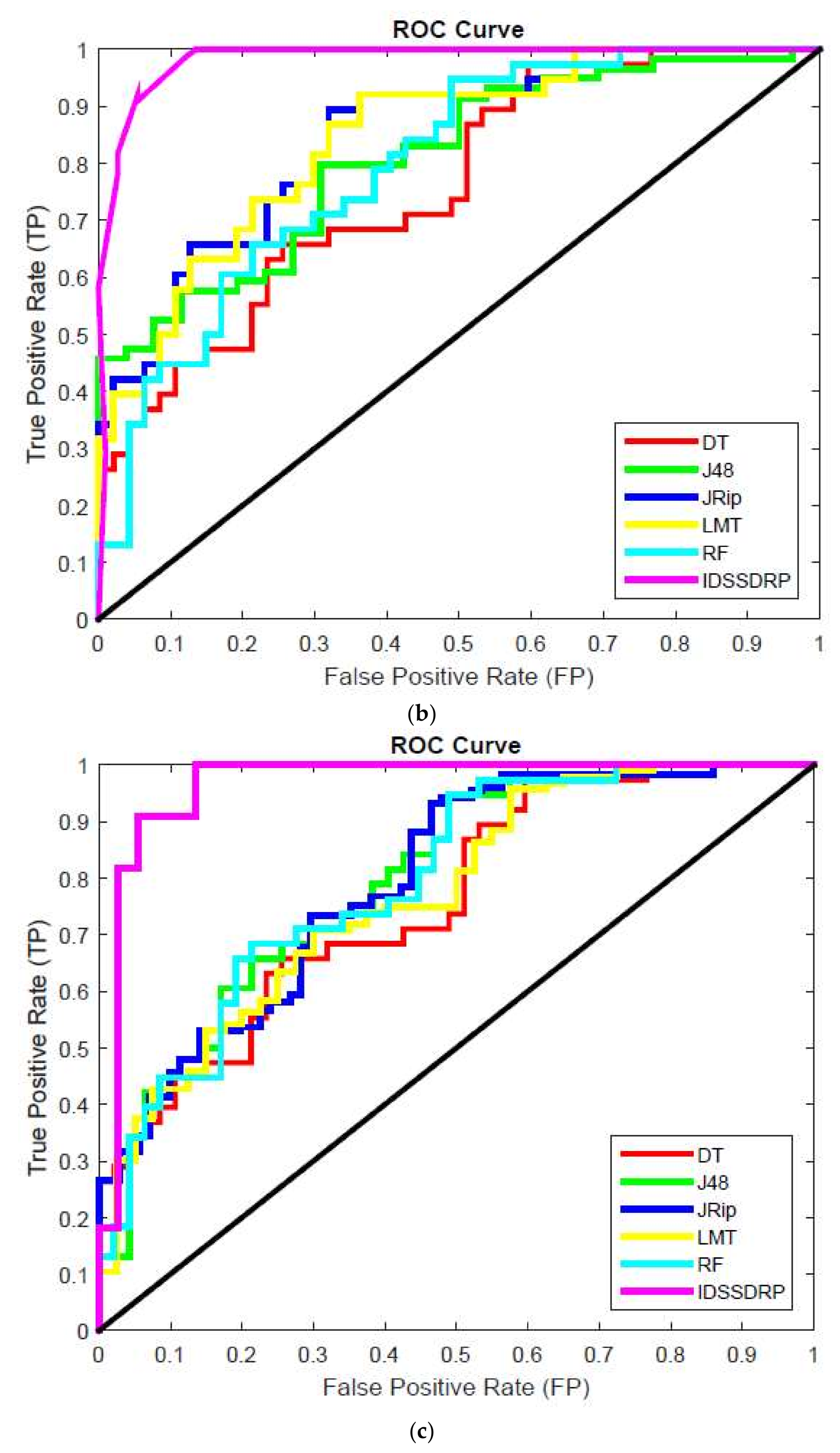
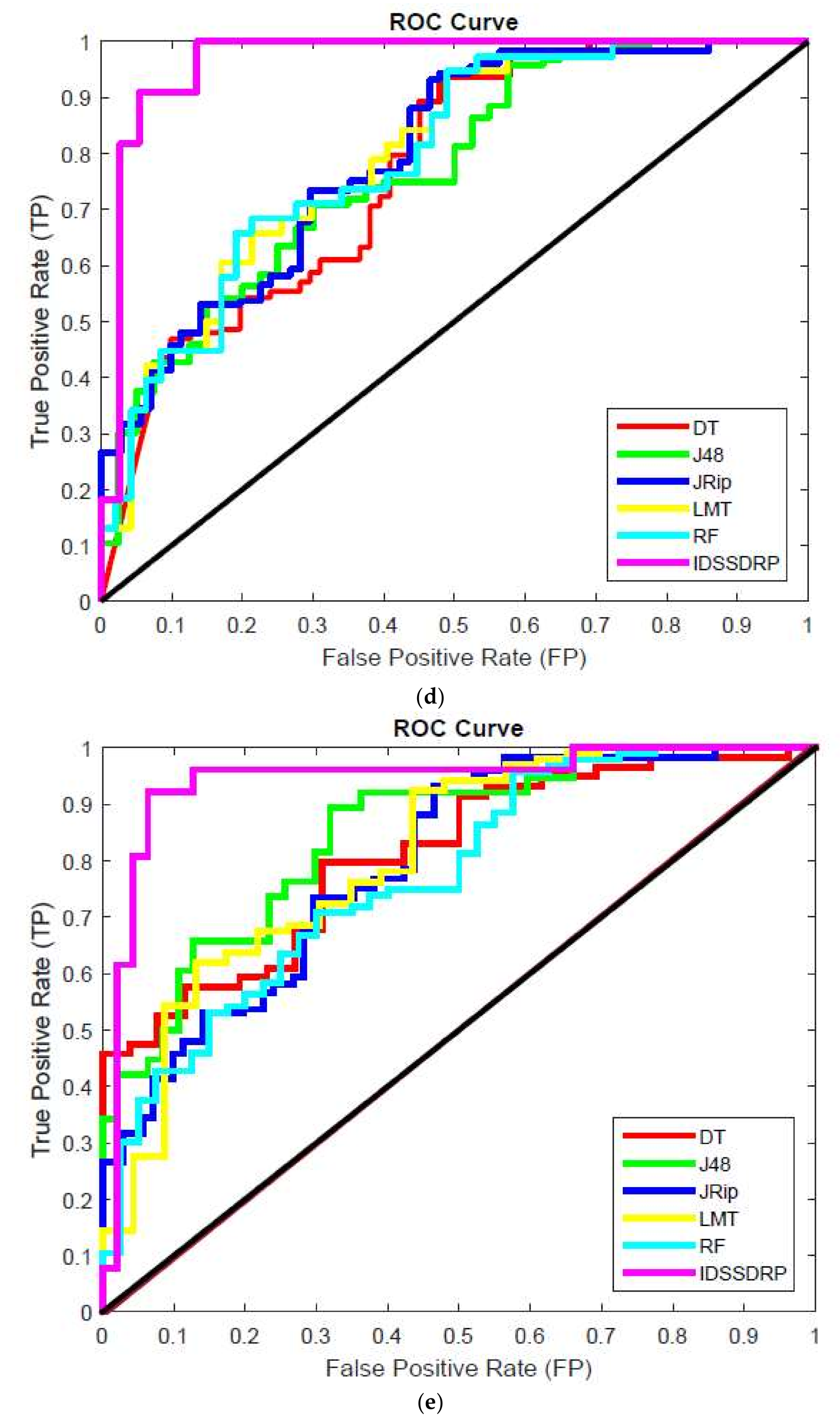
The receiver operating characteristic (ROC) curve is a chart plotting the various cut values of true positive rate towards the false positive rate. It is very important to investigate the performance of the various classifiers. ROC graphs are widely used in the field of decision rules making, machine learning, data analytics, and data mining analysis [57]. In this work, ROC curves for better superiority of soft set-based decision-making can be conducted. The decision-making rules for algorithms appear in the top left corner of the ROC space, which means that the model forecasts the class precisely. The diagonal line denotes the strategy of randomly predicting a class. Any classifier that appears at the bottom right of the ROC graph performs worse than random predictions. The data on the far-left side of the ROC graph is now getting more important.
Figure 10a–e shows the ROC curve analysis of the proposed IDSSDRP and the existing decision-making algorithms. The ROC curve evaluates the graphical performance of the proposed improved dominance soft set-based decision rules making with the pruning algorithm (IDSSDRP). With respect to all the datasets, i.e., GLCM_0, GLCM_45, GLCM_90, GLCM_13, and shape and color, the proposed decision-making algorithm performed much better than the other existing classification algorithms. The curve of the IDSSDRP algorithm appears in the top left border of the ROC graph. This means that the proposed approach correctly diagnosis the blast and non-blast cells.

6. Conclusions and Future Scope

In this paper, a novel improved dominance soft set-based decision rules generation with pruning algorithm (IDSSDRP) is proposed to predict the acute lymphoblastic leukemia images. The proposed method contains the following advantages. (1) Features are reduced using dominance soft set with AND operation in multi-soft set theory. This improves the classification accuracy and reduces the memory space. (2) Generated decision rules are utilized to predict the blast and non-blast cells. (3) The rule pruning algorithm simplifies the generated decision rules which helps to increase the computational speed. The empirical results show that the proposed IDSSDRP algorithm effectively predicts the tumor cells in ALL leukemia images. The ROC curve analysis precisely displays the proposed system’s performance in the accurate diagnosis of the disease.
In the future, we are preparing to create a hybrid method by combining the advantages of certain evolutionary algorithms, such as firefly optimization, gray wolf optimization, mouth flame, Lloyd’s algorithm, Huffman algorithm, etc., and set theory extensions.

Author Contributions

Conceptualization, G.J., H.H.I., A.T.A.; Data curation, N.A.K., K.M.F.; Formal analysis, G.J., H.H.I., A.T.A., A.K., N.A.K., K.M.F.; Supervision, H.H.I., A.T.A.; Funding acquisition, A.T.A., A.K.; Methodology, G.J., H.H.I., A.T.A.; Resources, N.A.K., K.M.F., A.K.; Software, H.H.I., G.J.; Investigation, A.T.A., A.K., N.A.K., K.M.F.; Validation, A.K., N.A.K., K.M.F.; Visualization, G.J., A.K., N.A.K., K.M.F.; Writing—original draft, G.J., H.H.I., A.T.A.; Writing—review & editing, G.J., H.H.I., A.T.A., A.K., N.A.K., K.M.F. All authors have read and agreed to the published version of the manuscript.

Funding

This research is funded by Prince Sultan University, Riyadh, Saudi Arabia.

Acknowledgments

The authors would like to thank Prince Sultan University, Riyadh, Saudi Arabia for supporting and funding this work. Special acknowledgment to Robotics and Internet-of-Things Lab (RIOTU) at Prince Sultan University, Riyadh, SA. Also, the authors wish to acknowledge the editor and anonymous reviewers for their insightful comments, which have improved the quality of this publication

Conflicts of Interest

The authors declare no conflict of interest.

Appendix A

Figure A1. Derived rules using IDSSDRP algorithm.
Electronics 09 00794 g0a1aElectronics 09 00794 g0a1b

Appendix B

Figure A2. Pruned rules.
Electronics 09 00794 g0a2

References

  1. National Cancer Institute (NCI): Division of Cancer Control and Population Sciences (DCCPS), Surveillance Research Program (SRP). Available online: https://seer.cancer.gov/statfacts/html/leuks.html (accessed on 11 April 2020).
  2. Arora, R.S.; Arora, B. Acute leukemia in children: A review of the current Indian data. South Asian J. Cancer 2016, 5, 155–160. [Google Scholar] [CrossRef]
  3. NCRP Annual Reports. Available online: http://www.ncrpindia.org (accessed on 11 April 2020).
  4. Mohapatra, S.; Patra, D.; Satpathy, S. An ensemble classifier system for early diagnosis of acute lymphoblastic leukemia in blood microscopic images. Neural Comput. Appl. 2014, 24, 1887–1904. [Google Scholar] [CrossRef]
  5. Kennedy, J.; Eberhart, R. Particle swarm optimization (PSO). In Proceedings of the IEEE International Conference on Neural Networks, Perth, Australia, 27 November–1 December 1995; pp. 1942–1948. [Google Scholar] [CrossRef]
  6. Zhang, Y.; Huang, D.; Ji, M.; Xie, F. Image segmentation using PSO and PCM with Mahalanobis distance. Expert Syst. Appl. 2011, 38, 9036–9040. [Google Scholar] [CrossRef]
  7. Benaichouche, A.N.; Oulhadj, H.; Siarry, P. Improved spatial fuzzy c-means clustering for image segmentation using PSO initialization, Mahalanobis distance and post-segmentation correction. Digit. Signal Process. 2013, 23, 1390–1400. [Google Scholar] [CrossRef]
  8. Chander, A.; Chatterjee, A.; Siarry, P. A new social and momentum component adaptive PSO algorithm for image segmentation. Expert Syst. Appl. 2011, 38, 4998–5004. [Google Scholar] [CrossRef]
  9. Omran, M.G.; Engelbrecht, A.P.; Salman, A. Image classification using particle swarm optimization. Recent Adv. Simulated Evol. Learn. 2004, 347–365. [Google Scholar] [CrossRef]
  10. Inbarani, H.H.; Azar, A.T.; Jothi, G. Supervised hybrid feature selection based on PSO and rough sets for medical diagnosis. Comput. Methods Programs Biomed. 2014, 113, 175–185. [Google Scholar] [CrossRef]
  11. Wahhab, H.T.A. Classification of Acute Leukemia Using Image Processing and Machine Learning: Techniques. Ph.D. Thesis, University of Malaya, Kuala Lumpur, Malaysia, 2015. [Google Scholar]
  12. Molodtsov, D. Soft set theory—First results. Comput. Math. Appl. 1999, 37, 19–31. [Google Scholar] [CrossRef] [Green Version]
  13. Maji, P.K.; Roy, A.R.; Biswas, R. An application of soft sets in a decision-making problem. Comput. Math. Appl. 2002, 44, 1077–1083. [Google Scholar] [CrossRef] [Green Version]
  14. Hassanien, A.E.; Ali, J.M. Rough set approach for generation of classification rules of breast cancer data. Informatica 2004, 15, 23–38. [Google Scholar] [CrossRef]
  15. Du, W.S.; Hu, B.Q. Dominance-based rough fuzzy set approach and its application to rule induction. Eur. J. Oper. Res. 2017, 261, 690–703. [Google Scholar] [CrossRef]
  16. Isa, A.M.; Rose, A.N.M.; Deris, M.M. Dominance-based soft set approach in decision-making analysis. In Lecture Notes in Computer Science, Proceedings of the Advanced Data Mining and Applications, Beijing, China, 17–19 December 2011; Tang, J., King, I., Chen, L., Wang, J., Eds.; Springer: Berlin/Heidelberg, Germany, 2011; Volume 7120, p. 7120. [Google Scholar]
  17. Ma, X.; Liu, Q.; Zhan, J. A survey of decision-making methods based on certain hybrid soft set models. Artif. Intell. Rev. 2017, 47, 507–530. [Google Scholar] [CrossRef] [Green Version]
  18. Karaaslan, F. Possibility neutrosophic soft sets and PNS-decision making method. App. Soft Comp. 2017, 54, 403–414. [Google Scholar] [CrossRef] [Green Version]
  19. Kumar, S.U.; Inbarani, H.H.; Kumar, S.S. Bijective soft set based classification of medical data. In Proceedings of the 2013 International Conference on Pattern Recognition, Informatics and Mobile Engineering, Salem, India, 21–22 February 2013; pp. 517–552. [Google Scholar] [CrossRef]
  20. Zhan, J.; Ali, M.I.; Mehmood, N. On a novel uncertain soft set model: Z-soft fuzzy rough set model and corresponding decision making methods. Appl. Soft Comput. 2017, 56, 446–457. [Google Scholar] [CrossRef]
  21. Zhan, J.; Liu, Q.; Herawan, T. A novel soft rough set: Soft rough hemirings and corresponding multicriteria group decision making. Appl. Soft Comput. 2017, 54, 393–402. [Google Scholar] [CrossRef]
  22. Putzu, L.; Caocci, G.; Di Ruberto, C. Leucocyte classification for leukaemia detection using image processing techniques. Artif. Intell. Med. 2014, 62, 179–191. [Google Scholar] [CrossRef] [Green Version]
  23. Jothi, G.; Inbarani, H.H.; Azar, A.T.; Almustafa, K.M. Feature Reduction based on Modified Dominance Soft Set. In Proceedings of the 5th International Conference on Fuzzy Systems and Data Mining (FSDM2019), Kitakyushu City, Japan, 19–21 October 2019; pp. 261–272. [Google Scholar]
  24. Inbarani, H.H.; Azar, A.T.; Jothi, G. Leukemia image segmentation using a hybrid histogram-based soft covering rough k-means clustering algorithm. Electronics 2020, 9, 188. [Google Scholar] [CrossRef] [Green Version]
  25. Mishra, S.; Majhi, B.; Sa, P.K. Texture feature-based classification on microscopic blood smear for acute lymphoblastic leukemia detection. Biomed. Signal Process. Control 2019, 47, 303–311. [Google Scholar] [CrossRef]
  26. Jothi, G.; Inbarani, H.H.; Azar, A.T.; Devi, K.R. Rough set theory with Jaya optimization for acute lymphoblastic leukemia classification. Neural Comput. Appl. 2019, 31, 5175–5194. [Google Scholar] [CrossRef]
  27. Al-jaboriy, S.S.; Sjarif, N.N.A.; Chuprat, S.; Abduallah, W.M. Acute lymphoblastic leukemia segmentation using local pixel information. Pattern Recognit. Lett. 2019, 125, 85–90. [Google Scholar] [CrossRef]
  28. Negm, A.S.; Hassan, O.A.; Kandil, A.H. A decision support system for acute leukaemia classification based on digital microscopic images. Alex. Eng. J. 2018, 57, 2319–2332. [Google Scholar] [CrossRef]
  29. Labati, R.D.; Piuri, V.; Scotti, F. All-IDB: The acute lymphoblastic leukemia image database for image processing. In Proceedings of the 18th IEEE International Conference on Image Processing, Brussels, Belgium, 11–14 September 2011; pp. 2045–2048. [Google Scholar]
  30. Scotti, F. Robust segmentation and measurements techniques of white cells in blood microscope images. In Proceedings of the IEEE Instrumentation and Measurement Technology Conference Proceedings, Sorrento, Italy, 24–27 April 2006; pp. 43–48. [Google Scholar]
  31. Scotti, F. Automatic morphological analysis for acute leukemia identification in peripheral blood microscope images. In Proceedings of the IEEE International Conference on Computational Intelligence for Measurement Systems and Applications, Messian, Italy, 20–22 July 2005; pp. 96–101. [Google Scholar]
  32. Piuri, V.; Scotti, F. Morphological classification of blood leucocytes by microscope images. In Proceedings of the IEEE International Conference on Computational Intelligence for Measurement Systems and Applications, Boston, MA, USA, 14–16 July 2004; pp. 103–108. [Google Scholar]
  33. Prabu, G.; Inbarani, H.H. PSO for acute lymphoblastic leukemia classification in blood microscopic images. Indian J. Eng. 2015, 12, 146–151. [Google Scholar]
  34. Jati, A.; Singh, G.; Mukherjee, R.; Ghosh, M.; Konar, A.; Chakraborty, C.; Nagar, A.K. Automatic leukocyte nucleus segmentation by intuitionistic fuzzy divergence based thresholding. Micron 2014, 58, 55–65. [Google Scholar] [CrossRef] [PubMed]
  35. El-Baz, A.; Jiang, X.; Suri, J.S. Biomedical Image Segmentation: Advances and Trends; CRC Press: Boca Raton, FL, USA, 2016. [Google Scholar]
  36. Haralick, R.M.; Shanmugam, K. Textural features for image classification. IEEE Trans. Syst. Man Cybern. 1973, 6, 610–621. [Google Scholar] [CrossRef] [Green Version]
  37. Soh, L.K.; Tsatsoulis, C. Texture analysis of SAR sea ice imagery using gray level co-occurrence matrices. IEEE Trans. Geosci. Remote Sens. 1999, 37, 780–795. [Google Scholar] [CrossRef] [Green Version]
  38. Clausi, D.A. An analysis of co-occurrence texture statistics as a function of grey level quantization. Can. J. Remote Sens. 2002, 28, 45–62. [Google Scholar] [CrossRef]
  39. Jothi, G.; Inbarani, H.H. Hybrid tolerance rough set–firefly based supervised feature selection for MRI brain tumor image classification. Appl. Soft Comput. 2016, 46, 639–651. [Google Scholar]
  40. Alsalem, M.A.; Zaidan, A.A.; Zaidan, B.B.; Hashim, M.; Madhloom, H.T.; Azeez, N.D.; Alsyisuf, S. A review of the automated detection and classification of acute leukaemia: Coherent taxonomy, datasets, validation and performance measurements, motivation, open challenges and recommendations. Comput. Methods Prog. Biomed. 2018, 158, 93–112. [Google Scholar] [CrossRef]
  41. Jothi, G.; Inbarani, H.H.; Azar, A.T. Hybrid tolerance rough set: PSO based supervised feature selection for digital mammogram images. Int. J. Fuzzy Syst. Appl. 2013, 3, 15–30. [Google Scholar] [CrossRef] [Green Version]
  42. Jothi, G.; Inbarani, H.H. Soft set based feature selection approach for lung cancer. Int. J. Sci. Eng. Res. 2012, 3, 1–7. [Google Scholar]
  43. Herawan, T.; Deris, M.M. On multi-soft sets construction in information systems. In Emerging Intelligent Computing Technology and Applications. With Aspects of Artificial Intelligence, Lecture Notes in Computer Science, ICIC 2009, Ulsan, South Korea, 16–19 September 2009; Huang, D.S., Jo, K.H., Lee, H.H., Kang, H.J., Bevilacqua, V., Eds.; Springer: Berlin/Heidelberg, Germany, 2009; Volume 5755. [Google Scholar]
  44. Herawan, T.; Rose, A.N.M.; Mat Deris, M. Soft set theoretic approach for dimensionality reduction. In Database Theory and Application. DTA 2009, Communications in Computer and Information Science; Slezak, D., Kim, T., Zhang, Y., Ma, J., Chung, K., Eds.; Springer: Berlin/Heidelberg, Germany, 2009; Volume 64. [Google Scholar]
  45. Mitchell, T.M. Machine Learning; McGraw Hill: Burr Ridge, IL, USA, 1997; Volume 45, pp. 870–877. [Google Scholar]
  46. Quinlan, J.R. C4. 5: Programs for Machine Learning, Morgan Kaufmann Series in Machine Learning; Elsevier: Amsterdam, The Netherlands, 1993. [Google Scholar]
  47. Cohen, W.W. Fast effective rule induction. In Proceedings of the Twelfth International Conference on Machine Learning, Tahoe City, CA, USA, 9–12 July 1995; pp. 115–123. [Google Scholar]
  48. Landwehr, N.; Hall, M.; Frank, E. Logistic model trees. Mach. Learn. 2005, 59, 161–205. [Google Scholar] [CrossRef] [Green Version]
  49. Liaw, A.; Wiener, M. Classification and regression by random. For. R News 2002, 2, 18–22. [Google Scholar]
  50. Bekkar, M.; Djemaa, H.K.; Alitouche, T.A. Evaluation measures for models assessment over imbalanced data sets. J. Inf. Eng. Appl. 2013, 3, 27–38. [Google Scholar]
  51. Sokolova, M.; Lapalme, G. A systematic analysis of performance measures for classification tasks. Inf. Process. Manag. 2009, 45, 427–437. [Google Scholar] [CrossRef]
  52. Demšar, J. Statistical comparisons of classifiers over multiple data sets. J. Mach. Learn. Res. 2006, 7, 1–30. [Google Scholar]
  53. Ganesan, J.; Inbarani, H.H.; Azar, A.T.; Polat, K. Tolerance rough set firefly-based quick reduct. Neural Comp. Appl. 2017, 28, 2995–3008. [Google Scholar] [CrossRef]
  54. Sayed, G.I.; Hassanien, A.E.; Azar, A.T. Feature selection via a novel chaotic crow search algorithm. Neural Comp. Appl. 2019, 31, 171–188. [Google Scholar] [CrossRef]
  55. Inbarani, H.H.; Kumar, S.U.; Azar, A.T.; Hassanien, A.E. Hybrid rough-bijective soft set classification system. Neural Comp. Appl. 2018, 29, 67–78. [Google Scholar] [CrossRef]
  56. Kumar, S.S.; Inbarani, H.H.; Azar, A.T.; Polat, K. Covering-based rough set classification system. Neural Comp. Appl. 2017, 28, 2879–2888. [Google Scholar] [CrossRef]
  57. Fawcett, T. An introduction to ROC analysis. Pattern Recognit. Lett. 2006, 27, 861–887. [Google Scholar] [CrossRef]
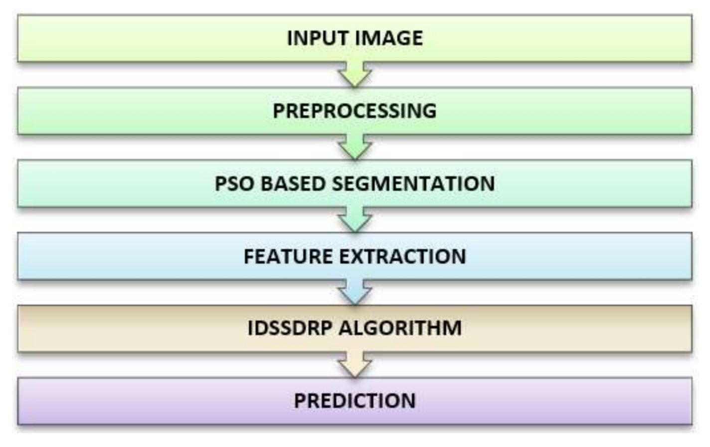
Figure 1. Proposed system architecture.
Electronics 09 00794 g001
Figure 2. L*A*B colour conversion outputs.
Electronics 09 00794 g002
Figure 3. Segmentation results using PSO. as (a) Im114_1, Im070_1 and Im073_1; (b) Im192_0, Im259_0 and Im248_0; (c) Im001_1, Im002_1 and Im018_1; (d) Im056_1, Im057_1 and Im060_1.
Electronics 09 00794 g003aElectronics 09 00794 g003b
Figure 4. Extracted features.
Electronics 09 00794 g004
Figure 5. Reduction percentage for various IDSSDRP.
Electronics 09 00794 g005
Figure 6. Performance of rule pruning algorithm.
Electronics 09 00794 g006
Figure 7. Comparison of overall prediction accuracies.
Electronics 09 00794 g007
Figure 8. Prediction error rate.
Electronics 09 00794 g008
Figure 9. Evaluation of various prediction metrics.
Electronics 09 00794 g009aElectronics 09 00794 g009b
Figure 10. ROC curve analysis. as (a) IDSSDRP method - GLCM_0; (b) IDSSDRP method - GLCM_45; (c) IDSSDRP method - GLCM_90; (d) IDSSDRP method - GLCM_135; (e) IDSSDRP method - Shape and Colour.
Electronics 09 00794 g010aElectronics 09 00794 g010bElectronics 09 00794 g010c
Table 1. Sample dataset.
Candidatea1
(Degree)
a2
(Work_Experience)
a3
(German_Lang)
a4
(Personality)
d
Decision_Class
1MBAMediumKnownExcellentAccept
2MBALowKnownNormalReject
3M.ScLowKnownGoodReject
4MCAHighKnownNormalAccept
5MCAMediumKnownNormalReject
6MCAHighKnownExcellentAccept
7MBAHighUnknownGoodAccept
8M.ScLowUnknownExcellentReject
Table 2. Multi-value information system.
a1a2a3a4d
MBAM.ScMCAMediumLowHighKnownUnknownExcellentNormalGoodAcceptReject
1001001010010
1000101001001
0100101000101
0010011001010
0011001001001
0010011010010
1000010100110
0100100110001
Table 3. Acquired Reducts using IDSSA.
DatasetNo. of Features ExtractedIDSSA
GLCM_02210
GLCM_452211
GLCM_902211
GLCM_1352211
Shape and Colour2212
Table 4. Confusion Matrix.
DescriptionResults Obtained for Confusion Matrix
Actual Output-Predicted OutputDTJ48JRipLMTRFProposed
Healthy Image (HI)Unhealthy Image (UI)HIUIHIUIHIUIHIUIHIUIHIUI
Healthy ImageCorrectly Predicted as Healthy Image (TP)Incorrectly Predicted as Unhealthy Image (FN)119561225311461122531066816213
Unhealthy ImageIncorrectly Predicted as Healthy Image (FP)Correctly Predicted as Unhealthy Image (TN)1318014179141791417921913190
Table 5. Detailed interpretations for various classification measures.
MetricsExplanationEquation
Sensitivity
(or Recall)
(in %)
It is employed to measure the True positive rates TP / TP   +   FN
Specificity
(in %)
Measure the true negative rates TN / TN   +   FP
Accuracy
(in %)
Calculate the probability of the true value of the class attributes. TP + TN / TP + TN + FP + FN
Precision
(in %)
Degree of exactness TP / TP   +   FP
F1 scoreThe harmonic mean of precision and recall 2 × Precision   ×   Recall / Precision   +   Recall
Error Rate
(=1 − accuracy)
An approximation of misclassification probability. FP + FN / TP + TN + FP + FN
Matthews Correlation
Coefficient (MCC)
The association between the actual and predicted class TP   ×   TN FP   ×   FN TP   + FP × TP   +   FN × TN   +   FP × TN   +   FN
LiftThe proportion among the outcomes obtained with and without the Model TP / TP + FP / TP + FN / TP + TN + FP + FN
G-meanThe product of the prediction accuracies for both classes precison   × recall
Youden’s indexThe arithmetic mean among sensitivity and specificity sensitivity   +   specificity     1
Balanced Classification Rate (BCR)The mean of sensitivity and specificity. ½ sensitivity   +   specificity
Balanced Error Rate (BER)or The mean of the errors in each class. It also named as Half Total Error Rate (HTER) 1     BCR
Note: TN-True Positive; TP-True Negative; FP- False Positive; FN-False Negative.
Table 6. GLCM_0 dataset.
Prediction MetricsDecision TreeJ48JRipLMTRandom ForestProposed
Accuracy 79.8179.8178.3778.8578.3798.08
Sensitivity 94.5294.5297.2693.8493.8498.63
Specificity 45.1645.1633.8743.5541.9496.77
Precision 80.2380.2377.6079.6579.1998.63
Error Rate0.200.200.220.210.220.02
MCC0.480.480.440.450.440.95
F1 measure86.7986.7986.3286.1685.8998.63
G-mean87.0887.0886.8786.4586.2098.63
Lift value1.141.141.111.131.131.41
Youden’s index0.400.400.310.370.360.95
BCR 69.8469.8465.5768.6967.8997.70
BER0.300.300.340.310.320.02
Table 7. GLCM_45 dataset.
Prediction MetricsDecision TreeJ48JRipLMTRandom ForestProposed
Accuracy77.8878.8579.3379.8178.8597.12
Sensitivity92.4797.2692.4792.4793.1597.26
Specificity43.5535.4848.3950.0045.1696.77
Precision79.4178.0280.8481.3380.0098.61
Error Rate0.220.210.210.200.210.03
MCC0.430.450.470.480.450.93
F1 measure85.4486.5986.2686.5486.0897.93
G-mean85.6987.1186.4686.7286.3397.93
Lift value1.131.111.151.161.141.40
Youden’s index0.360.330.410.420.380.94
BCR68.0166.3770.4371.2369.1697.02
BER0.320.340.300.290.310.03
Table 8. GLCM_90 dataset.
Prediction MetricsDecision TreeJ48JRipLMTRandom ForestProposed
Accuracy81.2581.2581.2582.2182.2199.04
Sensitivity96.5896.5896.5897.2697.2699.32
Specificity45.1645.1645.1646.7746.7798.39
Precision80.5780.5780.5781.1481.1499.32
Error Rate0.190.190.190.180.180.01
MCC0.520.520.520.550.550.98
F1 measure87.8587.8587.8588.4788.4799.32
G-mean88.2188.2188.2188.8488.8499.32
Lift value1.151.151.151.161.161.41
Youden’s index0.420.420.420.440.440.98
BCR70.8770.8770.8772.0272.0298.85
BER0.290.290.290.280.280.01
Table 9. GLCM_135 dataset.
Prediction MetricsDecision TreeJ48JRipLMTRandom ForestProposed
Accuracy79.8179.8179.8178.8576.9297.60
Sensitivity94.5294.5292.4791.1089.0498.63
Specificity45.1645.1650.0050.0048.3995.16
Precision80.2380.2381.3381.1080.2597.96
Error Rate0.200.200.200.210.230.02
MCC0.480.480.480.460.410.94
F1 measure86.7986.7986.5485.8184.4298.29
G-mean87.0887.0886.7285.9584.5398.29
Lift value1.141.141.161.161.141.40
Youden’s index0.400.400.420.410.370.94
BCR69.8469.8471.2370.5568.7196.90
BER0.300.300.290.290.310.03
Table 10. Shape and Colour dataset.
Prediction MetricsDecision TreeJ48JRipLMTRandom ForestProposed
Accuracy81.2581.7379.8181.7380.2995.67
Sensitivity96.5895.8992.4795.2192.4797.26
Specificity45.1648.3950.0050.0051.6191.94
Precision80.5781.4081.3381.7681.8296.60
Error Rate0.190.180.200.180.200.04
MCC0.520.540.480.540.500.90
F1 measure87.8588.0586.5487.9786.8296.93
G-mean88.2188.3586.7288.2386.9896.93
Lift value1.151.161.161.161.171.38
Youden’s index0.420.440.420.450.440.89
BCR70.8772.1471.2372.6072.0494.60
BER0.290.280.290.270.280.05
Table 11. Comparison of various classification algorithms performance.
Classification AlgorithmsAccuracySensitivitySpecificity
Existing Approach
NB80.9569.4988.4
KNN78.5779.5978.43
MLP78.5785.975.53
RBFN79.0564.1281.05
SVM91.4375.1398.7
GLCM_0 Dataset
Decision Tree79.8194.5245.16
J4879.8194.5245.16
JRip78.3797.2633.87
LMT78.8593.8443.55
Random Forest78.3793.8441.94
Proposed IDSSDRP98.0898.6396.77
GLCM_45 Dataset
Decision Tree77.8892.4743.55
J4878.8597.2635.48
JRip79.3392.4748.39
LMT79.8192.4750
Random Forest78.8593.1545.16
Proposed IDSSDRP97.1297.2696.77
GLCM_90 Dataset
Decision Tree81.2596.5845.16
J4881.2596.5845.16
JRip81.2596.5845.16
LMT82.2197.2646.77
Random Forest82.2197.2646.77
Proposed IDSSDRP99.0499.3298.39
GLCM_135 Dataset
Decision Tree79.8194.5245.16
J4879.8194.5245.16
JRip79.8192.4750
LMT78.8591.150
Random Forest76.9289.0448.39
Proposed IDSSDRP97.698.6395.16
Shape and Colour
Decision Tree81.2596.5845.16
J4881.7395.8948.39
JRip79.8192.4750
LMT81.7395.2150
Random Forest80.2992.4751.61
Proposed IDSSDRP95.6797.2691.94