Metamodelling Techniques for the Optimal Design of Low-Noise Amplifiers

Abstract

In this article we deal with the optimal sizing of low-noise amplifiers (LNAs) using newly proposed metamodeling techniques. The main objective is to construct metamodels of main performances of the LNAs (namely, the third intercept point (IIP3), the scattering parameters (S_ij), and the noise figure (NF)) and use them inside an optimization kernel for maximizing the circuits’ performances. The kriging surrogate modelling technique is used for constructing these models. The particle swarm optimization (PSO) technique is considered as the optimization metaheuristic. Two CMOS amplifiers are considered: a UMTS LNA and a multistandard LNA. Obtained results show that, at the considered working frequencies, the first LNA exhibits at 2.14 GHz a noise figure of 1.30 dB, an S₂₁ of 16.01 dB, an S₁₁ of −12.60 dB, and an IIP3 of 8.30 dBm. At 2 GHz, the second LNA has a noise figure of 1.24 dB, an S₂₁ of 17.16 dB, an S₁₁ of −13.74 dB, and an IIP3 of 4.30 dBm. Comparisons between results obtained using the constructed models and those of the simulation are presented to show the perfect agreement between them.

1. Introduction

The optimal design of analogue circuits has long been, and continues to be, a tedious and complicated task that depends significantly on the designer’s experience. It is indeed a subject of great interest to designers, engineers, researchers, etc. This is mainly due to the lack of dedicated design automation tools. Moreover, and as is well known, for radio frequency applications such a task is greatly complicated by the fact that additional parasitics/performances/constraints have to be taken into consideration in the design process (the most constraining being arguably the third intercept point).

In this work we are interested in the optimal design of low-noise amplifiers (LNAs).

The literature offers a plethora of research works that have dealt with the design of such amplifiers. Different approaches have been considered, mainly:

• The use of the conventional equation-based techniques, see for instance [1,2,3];
• The in-loop based approaches, see [4,5,6].

The majority of these works deal with the optimization of the scattering parameters that are introduced within an optimization kernel as performances and/or constraints. Only a few papers have considered the maximization of the third intercept point (IIP3) due to its high complexity [4,5,7,8]. Actually, IIP3 is generally considered as a circuit performance that is computed a posteriori, see for instance [4,8,9,10,11]. In [11], the authors have dealt with a symbolic approach for obtaining an approximation of the IIP3 expression. In [8] a graphical technique is used. It depicts the intercept point based on measurements of the fundamental and third-order intermodulation distortion amplitude for an input power sweep. Automating this measurement takes long computation times. The authors in [4] use another method: when the IIP3 is related to the direct current (DC) power consumption, the IIP3 is calculated in the region where the DC power consumption is below 60 dB (this region guarantees a linear relationship between the input and the output powers).

Recently, a new modelling technique has been proposed. It is known as ‘metamodelling’ or ‘surrogate modelling’. It has been shown and proven that such a technique can faithfully model complicated ‘non-linear’ phenomena using a relatively reduced input database [12,13,14,15,16,17]. It has overcome limitations and errors of the conventional modelling techniques [12]. Moreover, these metamodelling approaches offer additional very interesting features, namely the estimation of the error at the interpolation points. Different variants are available in the specialized literature:

• The polynomial regression model [13];
• The artificial neural network model [14];
• The kriging model [15];
• The radial basis function model [16];
• The support vector machine model and the support vector regression model [17].

Nowadays, metamodelling is used in many engineering domains: aeronautics [18], mechanics [19], electronics [20,21,22,23,24], telecommunication [25], and management science [26], to name a few.

The authors have already focused on the use of such techniques and have shown the efficiency of these modelling approaches for the design of some analogue circuits, see [20,21,22].

In this work we are interested in the design of high-performance low-noise amplifiers. The main objective is to model these circuits’ performances (namely IIP3, scattering parameters (S_ij), and noise figure (NF)) using the kriging technique. The constructed metamodels are then used within a particle swarm optimization (PSO)-based optimization kernel to generate the optimal values of the circuits’ parameters.

The rest of the paper is organized as follows. In Section 2, we provide an overview on the metamodelling techniques. In Section 3, we present the considered amplifiers and we deal with the construction and the validation of these circuits’ performance models. In Section 4, we consider the optimization approach, highlight the performances reached, and give comparisons with the simulation results. In Section 5, we conclude the work and underline some perspectives.

2. Overview of Surrogate Models

Surrogate modelling is a kind of an interpolation technique that, in contrast with the conventional approaches that focus on the linear regression term, deals with the error term by considering the correlation between the instances. It has rapidly become a popular method to solve the computation time problems related to constraint and performance evaluations [20,21,22,23,24,25,26,27,28,29,30,31]. Actually, it offers a very interesting advantage since, in many engineering applications, particularly in analogue circuit design, such evaluations/measures can be very time consuming, mainly when using an in-loop technique. For example, in [32] the sizing of integrated inductors is considered, and it is shown that, due to the electromagnetic simulations, it takes around two weeks to generate the Pareto front of three performances (Inductance/Area/Quality factor) of a square integrated inductor.

This new technique is capable of approximating very complex non-linear functions by a simple and an accurate model. A large number of works have used this method for modelling complex performances of analogue circuits, for example, in [30] the kriging model was used within a multi-objective robust optimization of electromagnetic devices. In [21], the authors have used the kriging modelling technique for the accurate approximation of several performances of a couple of circuits. In [22] the kriging model was combined with the PSO for optimizing the sizing of a current conveyor and a unity gain voltage amplifier. In [33], the response surface methodology is used within the multi-objective optimization in the aim to implement an accurate solution for the optimization of RF-MEMS switches. In [34], the authors used the support vector machine for standby statistical leakage estimation of CMOS circuits using sampling based methods, which your aim is to replace SPICE simulation with your proposed surrogate models.

In metamodelling, the interpolation function can be simplified and expressed as follows [27,32,35]:

$$Y(x)={\displaystyle \sum _{j=1}^N{\beta }_j}{f}_j(x)+Z(x)$$

(1)

where N is the number of sample points. fj(x) represents the j^th regression function model, β_j is the corresponding weighting coefficient, and Z(x) is a stochastic process. The latter has a mean value equal to zero, and the covariance between two sampling points x_i and x_j is expressed as [27,30,35]:

$$C\mathrm{ov}(Z(x_i),Z(x_j))={\sigma }^{2}R(R(\theta ,x_i,x_j))i,j=1........,N$$

(2)

where σ² is the variance coefficient of Z(x). R(θ,xi,xj) is the correlation function.

The most renowned correlation functions are:

• The spline correlation function:

$$R(\theta ,x_i,x_j)={\displaystyle {\prod }_{k=1}^N\max (0.1-{\theta }_k}{\left|x_i-x_j\right|}_k))$$

(3)

• The exponential correlation function:

$$R(\theta ,x_i,x_j)={\displaystyle {\prod }_{k=1}^N{e}^{-}{{}^{{\theta }_k}}^{({\left|x_i-x_j\right|}_k)}}$$

(4)

• The Gaussian correlation:

$$R(\theta ,x_i,x_j)={\displaystyle {\prod }_{k=1}^N{e}^{-}{{}^{{\theta }_k}}^{{({\left|x_i-x_j\right|}_k)}^2}}$$

(5)

where |.|_k is the distance between x_i and x_j in direction k. θ_k is the k^th element of the correlation parameters [27,30,35].

The best linear prediction of Y(x*) is defined as follows [27]:

$$\widehat{Y}(x^{*})={\beta }^{*}(\theta )+r(x^{*},\theta )R{(\theta )}^{-1}(Y-f{\beta }^{*}(\theta ))$$

(6)

where x* is the new sample, β* is the estimator of β, and Y is the (N*1) vector of the samples’ values, f is a unit vector (N*1), R is the correlation vector between x* and the N samples. The maximum probability estimation of β is defined as follows:

$${\beta }^{*}(\theta )={(f^{T}R{(\theta )}^{-1}f)}^{-1}(f^{T}R{(\theta )}^{-1}Y)$$

(7)

The accuracy of the prediction is expressed by the MSE predictor [26] (MSE stands for mean square error):

$$\widehat{s}(x^{*})={\widehat{\sigma }}^2(\theta )(1-r{R}^{-1}{r}^T+\frac{{(1-f^T{R}^{-1}{r}^T)}^2}{f^T{R}^{-1}f})$$

(8)

where

$${\widehat{\sigma }}^2=\frac{{(Y-f{\beta }^{*})}^T{R}^{-1}(Y-f{\beta }^{*})}{n}$$

(9)

It is to be mentioned that, when compared to the other modelling techniques, the kriging approach offers several advantages, such as the simplicity of its implementation, its accuracy, and the fact that it is able to provide an estimation of the model’s error [32,36]. The kriging technique using a Gaussian correlation function is adopted in this work.

3. On the Modelling of Low-Noise Amplifiers’ (LNAs) Performances

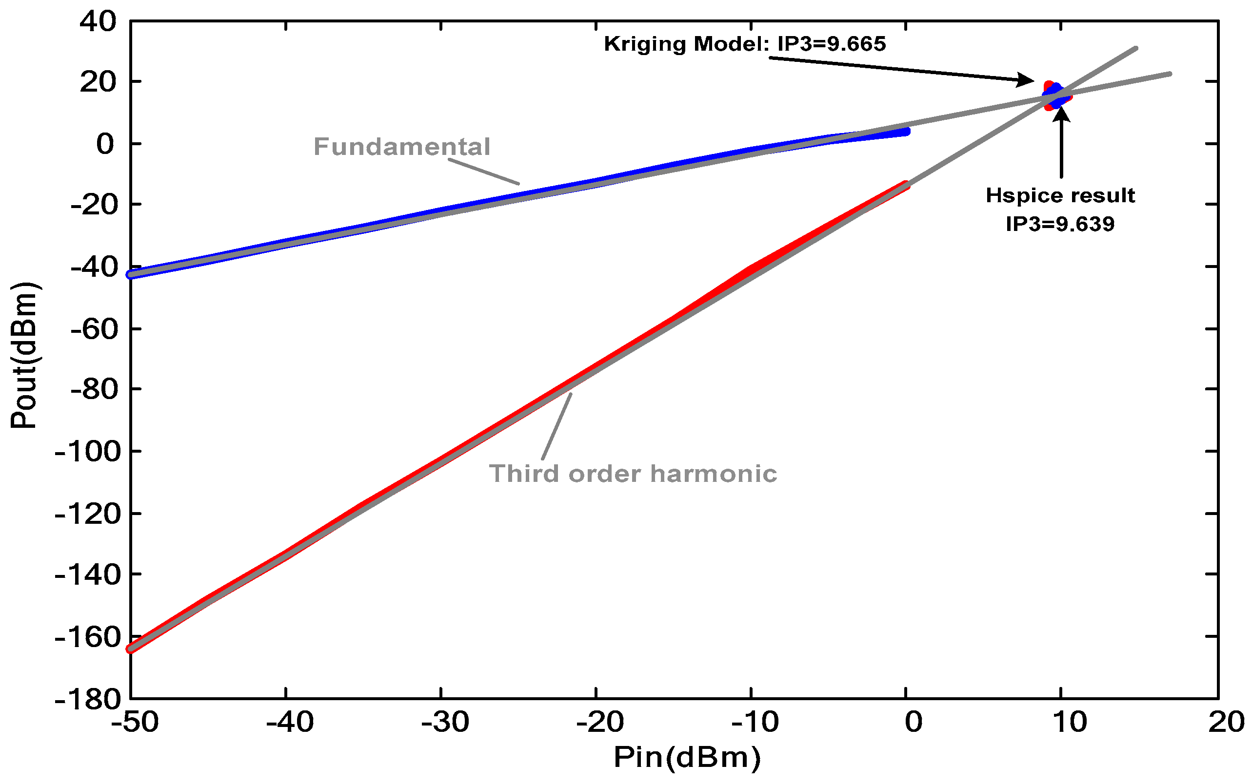
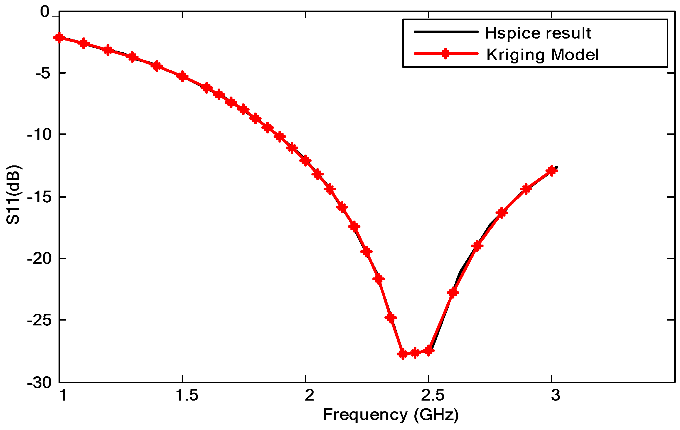
Radio frequency (RF) systems and circuits are key elements in various application domains such as mobile wireless communication, wireless local area network applications, mobile cellular, etc. [9,37].

In RF receivers, LNAs are arguably the most important circuits because their performances can considerably alter those of the rest of the system [2,38,39,40].

An LNA is characterized by several performances, principally its gain, its input and output matching (which can be evaluated via the scattering parameters S₂₁, S₁₁ and S₂₂), its noise figure (NF), and its third-order intercept point (IIP3).

As introduced above, two LNAs are considered in this work.

In the following, we present these circuits, deal with constructing models of the aforementioned performances, and present a comparison with Hspice [41] results for models’ validation purposes.

3.1. An UMTS LNA

Figure 1 presents a CMOS LNA, which topology was developed for UMTS applications, see [1,42]. R₁, R₂ and M₃ form the bias circuitry. M₂ forms the isolation stage between the input and the output of the circuit. L_L, R_L, and C_L form the circuit’s output impedance [1].

The kriging modelling technique is used for constructing models of the scattering parameters (S₂₁, S₁₁, S₂₂), the noise figure, and the third-order intercept point. Below, the models’ results are presented and compared with the Hspice simulation.

The adopted modelling approach encompasses four steps:

(1)

Design of Experiments: It consists of establishing a database that serves as an input for the kriging technique. This database is composed of the geometric variables of the considered circuits. The Latin hypercube sampling technique (LHS) is used for this purpose [43]; 1400 valid points were considered: 1200 samples for constructing the model and 200 test samples for checking/validating the model.

Table 1. Parameters’ ranges.

Components	Variation Ranges
W1, W2	[400 µm, 700 µm]
LL, L1	[0.1 nH, 1 nH]
L2	[5 nH, 10 nH]
CL, Cs	[5 pF, 10 pF]

gives details corresponding to the handled input variables, viz. MOS transistors channel widths and passive components values.

(2)

Performance Evaluation: Hspice simulator was used to evaluate the samples, check the constraints, and establish both databases. (.MEAS instruction within HSpice-RF was used to measure S_ij and NF values within the considered frequency range (it is to be mentioned that 30 models have constructed for each working frequency, in the range of 1 GHz to 3 GHz)).

(3)

Kriging associated to the Gaussian correlation function is used to construct the model.

(4)

Model Construction: It consists of applying the Gaussian correlation functions-based kriging technique to construct a model for each performance (S₁₁, S₂₂, S₂₁, NF and IIP3), using the established databases.

(5)

Model Validation: Both the root mean square error (RMSE) and the maximum absolute error (MAE) were considered to evaluate the accuracy of the constructed models. Corresponding equations are given by (10) and (11), where y_i and Y_i are the measured and the estimated performance values, respectively [44].

$$RMSE=\sqrt{\frac{1}{N}{\displaystyle \sum _{i=1}^N(y_i}-Y_i{)}^2}$$

(10)

$$MAE=\max \left|y_i-Y_i\right|$$

(11)

It is important to mention that one model has been generated for each working frequency (in the range of 1 GHz to 3 GHz). 30 models were constructed.

Table 2. Root mean square error (RMSE) for scattering parameters (S_ij) and noise figure (NF) of the UMTS LNA.

Frequency	S11	S22	S21	NF
1 GHz	0.0012 × 10−11	0.0001 × 10−11	0.0578 × 10−12	0.0386 × 10−13
1.5 GHz	0.0188 × 10−11	0.0037 × 10−11	0.0579 × 10−12	0.0208 × 10−13
2.14 GHz	0.6182 × 10−11	0.2809 × 10−11	0.1410 × 10−12	0.0369 × 10−13
2.5 GHz	0.1942 × 10−11	0.0514 × 10−11	0.1691 × 10−12	0.0652 × 10−13
3 GHz	0.0497 × 10−11	0.0046 × 10−11	0.0875 × 10−12	0.1328 × 10−13

and

Table 3. Maximum absolute error (MAE) for S_ij and NF of the UMTS LNA.

Frequency	S11	S22	S21	NF
1 GHz	0.0003 × 10−10	0.0003 × 10−11	0.1683 × 10−12	0.0822 × 10−13
1.5 GHz	0.0062 × 10−10	0.0133 × 10−11	0.1616 × 10−12	0.0488 × 10−13
2.14 GHz	0.3052 × 10−10	0.7127 × 10−11	0.3908 × 10−12	0.1066 × 10−13
2.5 GHz	0.0729 × 10−10	0.1689 × 10−11	0.5791 × 10−12	0.1910 × 10−13
3 GHz	0.0181 × 10−10	0.0156 × 10−11	0.3066 × 10−12	0.3730 × 10−13

give the errors’ values between the constructed models and Hspice results for five working frequencies. Figure 2, Figure 3, Figure 4, Figure 5 and Figure 6 depict the corresponding models and simulation results.

Regarding the third-order intercept point, one model was generated for each working input power (in the range of −50 dBm to 0 dBm). 10 models were constructed.

Table 4. RMSE and MAE error for third intercept point (IIP3) of the UMTS LNA.

Input Power	RMSE	MAE
−50 dBm	5.4793 × 10−13	3.1646 × 10−12
−40 dBm	4.1372 × 10−13	1.4415 × 10−12
−30 dBm	4.1928 × 10−13	1.4451 × 10−12
−20 dBm	3.9675 × 10−13	1.3305 × 10−12
−10 dBm	3.7601 × 10−13	1.3900 × 10−12

shows RMSE and MAE error values for the IIP3 in input powers.

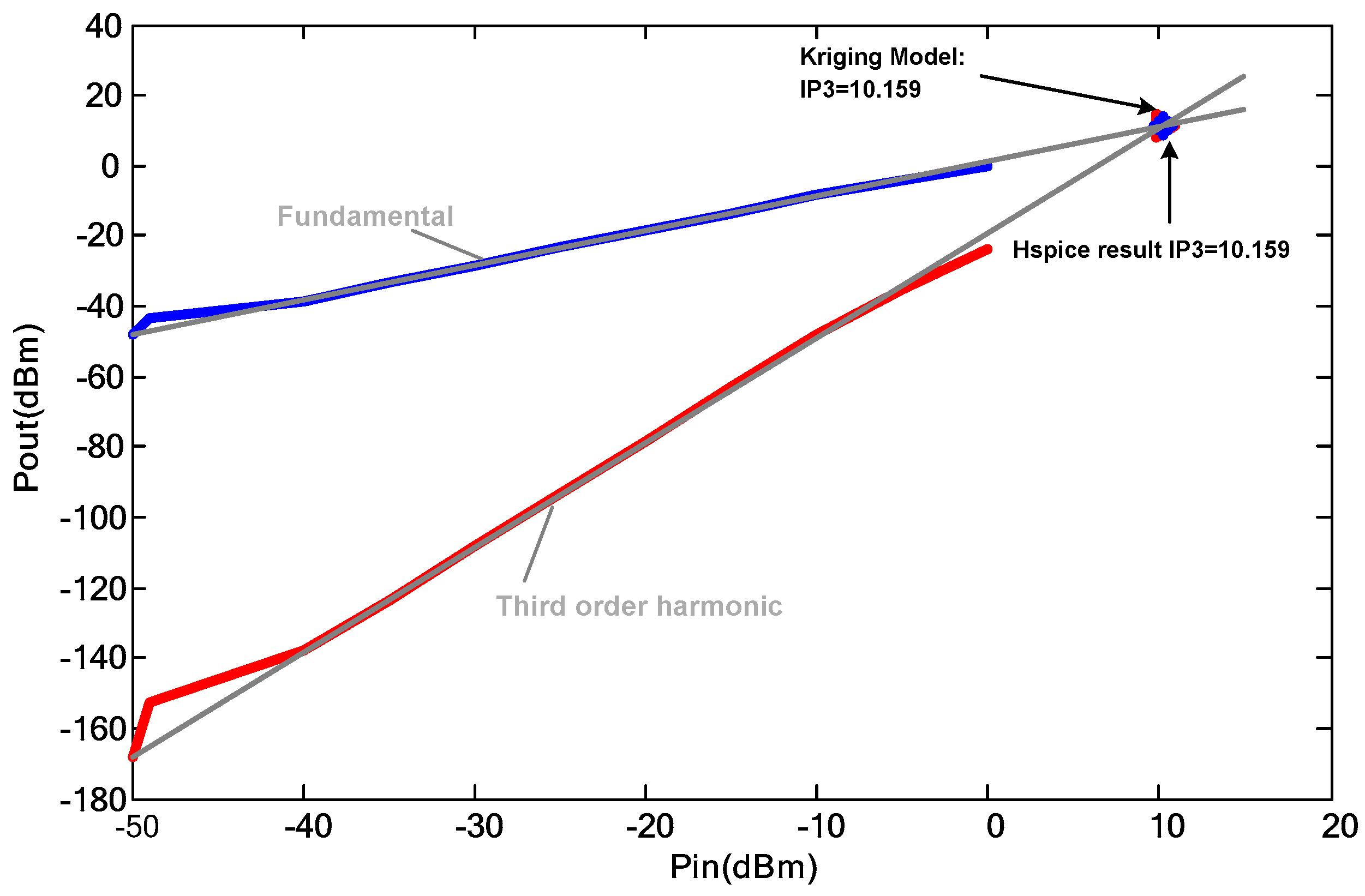
3.2. A Multistandard CMOS LNA

Figure 7 presents the CMOS transistor level schematic of a LNA for multistandard applications in the frequency range 1.5–2.5 GHz [1]. The proposed LNA design encompasses a cascade architecture for reducing the Miller effect and uses the reverse isolation. M₃, R₂, and R₁ form the biasing circuitry of the input transistor. L₂, C₁, and C₂ allow the input matching [1]. We refer the reader to [40] for further details regarding the LNA topologies and characteristics.

Constructed models of different performances of the multistandard-LNA are generated using the same approach adopted for the first application example. The database is composed of 10 input variables. Ranges of the geometric variables were set as indicated in

Table 5. Parameters’ ranges.

Components	Variation Ranges
W1, W2	[100 µm, 1000 µm]
LL	[0.5 nH, 0.9 nH]
L1	[0.01 nH, 0.9 nH]
L2	[1 nH, 10 nH]
CL, Cs	[1 pF, 10 pF]
C1, C2	[0.1 fF, 20 fF]
RL	[0.1 Ohm, 10 Ohm]

.

The kriging model was constructed using the Gaussian correlation function. 30 models were established.

Table 6. RMSE for S_ij and NF of the multistandard-LNA.

Frequency	S11	S22	S21	NF
1 GHz	0.0385 × 10−12	0.0244 × 10−12	0.0526 × 10−11	0.1767 × 10−13
1.5 GHz	0.3384 × 10−12	0.1694 × 10−12	0.0132 × 10−11	0.0953 × 10−13
2 GHz	0.7082 × 10−12	0.5271 ×10−12	0.0364 × 10−11	0.0881 × 10−13
2.5 GHz	0.8602 × 10−12	0.7183 × 10−12	0.1135 × 10−11	0.1729 × 10−13
3 GHz	0.7436 × 10−12	0.4882 × 10−12	0.0617 × 10−11	0.3702 × 10−13

and

Table 7. MAE for S_ij and NF of the multistandard-LNA.

Frequency	S11	S22	S21	NF
1 GHz	0.0184 ×10−11	0.0081 × 10−11	0.1692 × 10−11	0.0995 × 10−12
1.5 GHz	0.1908 × 10−11	0.0740 × 10−11	0.0448 × 10−11	0.0535 × 10−12
2.14 GHz	0.2519 × 10−11	0.1986 × 10−11	0.1430 × 10−11	0.0264 × 10−12
2.5 GHz	0.6047 × 10−11	0.3219 × 10−11	0.3684 × 10−11	0.0728 × 10−12
3 GHz	0.3300 × 10−11	0.2938 × 10−11	0.1963 × 10−11	0.1559 × 10−12

show the obtained error values for RMSE and MAE, respectively.

Table 8. RMSE and MAE for IIP3 of the multistandard-LNA.

Input Power	RMSE Error	MAE Error
−50 dBm	2.8713 × 10−12	6.9952 × 10−12
−40 dBm	3.6393 × 10−12	7.6232 × 10−12
−30 dBm	3.9481 × 10−12	10.7478 × 10−12
−20 dBm	1.4343 × 10−12	4.5812 × 10−12
−10 dBm	1.8178 × 10−12	5.8903 × 10−12

shows RMSE and MAE for IIP3 in input powers.

Figure 8, Figure 9, Figure 10, Figure 11 and Figure 12 show comparisons between simulation and model results.

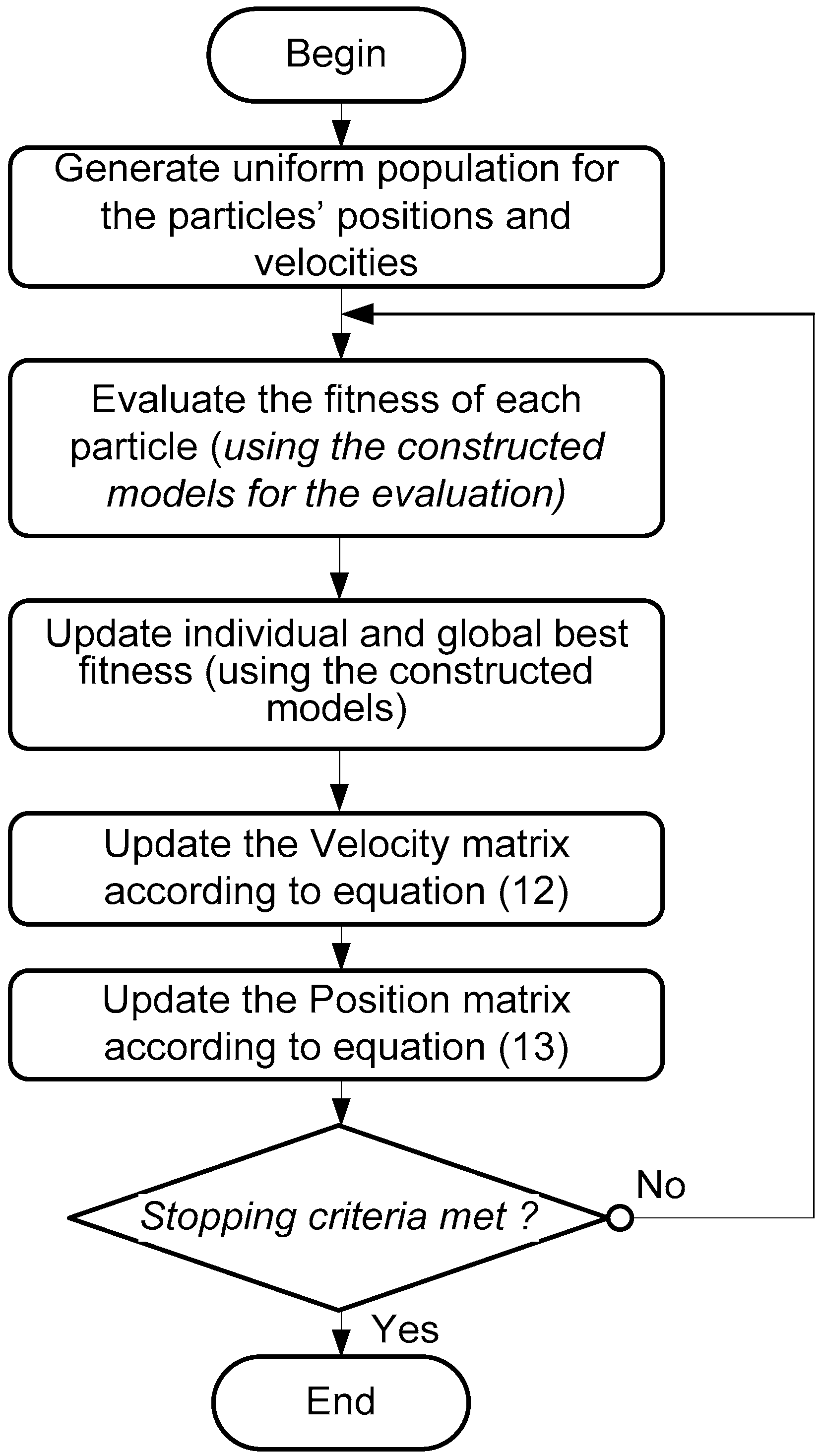
4. The Optimization Kernel

As introduced in Section 1, the constructed and validated metamodels of the LNAs’ performances are used within an optimization kernel for the optimal sizing of these circuits.

Figure 13 depicts the flowchart of the corresponding approach where the particle swarm optimization (PSO) metaheuristic is used as the optimization engine.

We briefly recall that PSO is a swarm intelligence technique. It has already been used in a plethora of applications in electronics engineering. It is a simple, robust and rapid metaheuristic. It mimics the behaviour of animals within swarms, namely fishes and birds [2,45,46,47]. Its mechanism works on updating each particle’s velocity and position at each iteration, according to the following equations:

$${ v \to }_i(t+1)=|\begin{array}{l}\omega { v \to }_i\left(t\right)\\ {+c}_{1}rand(0,1)(\overrightarrow{x_{Pbesti}}\left(t\right)-\overrightarrow{x_i}\left(t\right))\\ {+c}_{2}rand(0,1)(\overrightarrow{x_{Pbesti}}\left(t\right)-\overrightarrow{x_i}\left(t\right))\end{array}$$

(12)

$${\overrightarrow{x}}_i(t+1)={\overrightarrow{x}}_i(t)+{\overrightarrow{v}}_i(t)$$

(13)

where x_Pbest is the best position of particle i, x_Gbest is the global best position, w is the inertia weight of the particle. c₁ and c₂ are the constriction parameters.

In the following we provide optimization results for both circuits presented in the previous section. The considered working frequencies are 2.14 GHz and 2 GHz for the UMTS LNA and the multistandard LNA, respectively (AMS 0.35 μm CMOS technology (Level 49 model) is used.)

The optimization task consists of maximizing the third-order intercept point while imposing threshold constraints on the noise figure and on the S_ij parameters: NF < 4 dB, S₂₁ > 16 dB, S₁₁ < −10 dB and S₂₂ < −10 dB.

Regarding the PSO routine, the following parameters have been considered: 100 generations, 200 particles. The inertia weight is equal to 1, and both constriction parameters are equal to 2.

Table 9. Optimal parameters for the UMTS LNA.

W1 (µm)	W2 (µm)	LL (nH)	L2 (nH)	L1 (nH)	Cs (pF)	CL (pF)
482.30	620.61	0.948	7.432	0.244	8.648	5.187

and

Table 10. Optimal parameters’ values for the multistandard-LNA.

W1 (µm)	W2 (µm)	LL (nH)	L2 (nH)	L1 (nH)	Cs (pF)	C1 (fF)	C2 (fF)	RL (Ohm)	CL (pF)
574.57	494.82	0.859	7.910	0.303	2.903	9.865	2.074	0.346	6.731

give the optimal values obtained for the circuits’ components. Obtained performances are summarized in

Table 11. Optimal performances for the UMTS LNA with Pin = −50 dBm.

Performances	Specification	Kriging model-PSO	Hspice Simulation
S21(dB)	>16	16.013	16.093
S11(dB)	<−10	−12.600	−12.770
NF(dB)	<4	1.300	1.307
IIP3(dBm)	To be maximized	8.300	8.306

and

Table 12. Optimal performances of the multistandard-LNA with Pin = −50 dBm.

Performances	Specification	Kriging model-PSO	Hspice Simulation
S21(dB)	>16	17.165	17.164
S11(dB)	<−10	−13.735	−13.737
NF(dB)	<4	1.246	1.246
IIP3(dBm)	To be maximized	4.307	4.307

.

Regarding computation time, it is to be mentioned that for each constraint, namely, the scattering parameters and the noise figure, about 1 h 18 min was needed to evaluate the 1200 LHS samples and prepare the input database, and around 2 s for constructing the kriging model. The kriging-based PSO optimization routine took 44 s to maximize IIP3, which input database required 2 h 15 min to be prepared. For the sake of comparison, an inloop PSO-based optimization routine was considered to maximise the same performance under the same conditions, and it took 11 h 3 min 4 s to converge. (An Intel core I3-1.8 GHz-4Go RAM-64 bits PC was used).

5. Conclusions

An efficient approach to maximizing the IIP3 of low-noise amplifiers was presented. It consists of the use of surrogate models to construct models of circuits’ performances. This allows us to alleviate the burden related to the very long computation time when using the conventional in-loop optimization sizing processes where the simulator is used as the performance (and constraint) evaluator. The kriging metamodelling technique was used to construct accurate models of the IIP3, the noise figure and the scattering parameters. These models were used within a PSO-based optimization kernel for the optimal sizing of the LNAs. Comparisons with Hspice results were provided to show the perfect agreement between the simulated results and the expected ones.

The main objective of the paper is to present a fast way to evaluate LNA performances, particularly IIP3. The proposed approach can be extended to use complex models of integrated inductors such as those proposed in [32], and also sensitivity and yield analysis.

References

1. Garbaya, A.; Kotti, M.; Fakhfakh, M.; Siarry, P. The Backtracking Search for the Optimal Design of Low-Noise Amplifiers, In Computational Intelligence in Analog and Mixed-Signal. (AMS) and Radio-Frequency (RF) Circuit Design; Fakhfakh, M., Tlelo-Cuautle, E., Siarry, P., Eds.; Springer: Basel, Switzerland, 2015; pp. 391–412. [Google Scholar]
2. Kotti, M.; Sallem, A.; Bougharriou, M.; Fakhfakh, M.; Loulou, M. Optimizing CMOS LNA circuits through multi-objective meta-heuristics. In Proceedings of the International Workshop on Symbolic and Numerical Methods, Modeling and Applications to Circuit Design, Gammarth, Tunisia, 4–6 October 2010. [Google Scholar]
3. Neoh, S.C.; Marzuki, A.; Morad, N.; Lim, C.P.; Aziz, Z.A. An Interactive evolutionary algorithm for MMIC low noise amplifier design. ICIC Express Lett. 2009, 3, 15–19. [Google Scholar]
4. González-Echevarría, R.; Roca, E.; Castro-López, R.; Fernández, F.V.; Sieiro, J.; López-Villegas, J.M.; Vidal, N. An automated design methodology of RF circuits by using Pareto-optimal fronts of EM simulated inductors. IEEE Trans. Comput. Aided Des. Integr. Circuits Syst. 2016, 36, 15–26. [Google Scholar] [CrossRef] [Green Version]
5. Passos, F.; González-Echevarria, R.; Roca, E.; Castro-López, R.; Fernández, F.V. A two-step surrogate modeling strategy for single-objective and multi-objective optimization of radiofrequency circuits, methodologies and application. Soft Comput. 2019, 23, 4911–4925. [Google Scholar] [CrossRef] [Green Version]
6. Li, Y.; Yu, S.M.; Li, Y.L. A simulation-based hybrid optimization technique for low noise amplifier design automation. In Proceedings of the International Conference on Computational Science, Beijing, China, 27–30 May 2007. [Google Scholar]
7. Yadav, N.; Pandey, A.; Nath, V. Design of CMOS low noise amplifier for 1.57 GHz. In Proceedings of the International Conference on Microelectronics, Computing and Communications, Durgapur, India, 23–25 January 2016. [Google Scholar]
8. Lee, T.H. The Design of CMOS Radio-Frequency Integrated Circuits; Cambridge University Press: Cambridge, UK, 2003. [Google Scholar]
9. Misran, M.H.; MeorSaid, M.A.; Othman, M.A.; Ismail, M.M.; Sulaiman, H.A.; Cheng, K.G. Design of low noise amplifier using feedback and balanced technique for WLAN application. Procedia Eng. 2013, 53, 323–331. [Google Scholar] [CrossRef] [Green Version]
10. Arshad, S.; Ramzan, R.; Zafar, F.; Ul-Wahab, Q. Highly linear inductively degenerated 0.13 μm CMOS LNA using FDC technique. In Proceedings of the Asia Pacific Conference on Circuits and Systems, Ishigaki, Japan, 17–20 November 2014. [Google Scholar]
11. Tulunay, G.; Balkir, S. A synthesis tool for CMOS RF low noise amplifiers. IEEE Trans. Comput. Aided Des. Integr. Circuits Syst. 2008, 27, 977–982. [Google Scholar] [CrossRef]
12. Koziel, S.; Leifsson, L. Surrogate-Based Modeling and Optimization; Springer: New York, NY, USA, 2013. [Google Scholar]
13. Box, G.E.P.; Wilson, K.B. On the experimental attainment of optimum conditions. J. R. Stat. Soc. 1951, 13, 1–45. [Google Scholar] [CrossRef]
14. Yelten, M.B.; Franzon, P.D.; Steer, M.B. Comparison of modeling techniques in circuit variability analysis. Int. J. Numer. Modell. Electr. Net. Devices Fields 2012, 25, 288–302. [Google Scholar] [CrossRef]
15. Krige, D.G. A statistical approach to some basic mine valuation problems on the Witwatersrand. J. Chem. Metall. Min. Soc. South Afr. 1953, 52, 119–139. [Google Scholar]
16. Hardy, R.L. Multiquadratic equations of topography and other irregular surfaces. J. Geophys. Res. 1971, 76, 1905–1915. [Google Scholar] [CrossRef]
17. Zhou, Q.; Shao, X.; Jiang, P.; Zhou, H.; Shu, L. An adaptive global variable fidelity metamodeling strategy using a support vector regression based scaling function. Simul. Model. Pract. Theory 2015, 59, 18–35. [Google Scholar] [CrossRef]
18. Liao, Y.; Liu, L.; Long, T. Multi-objective aerodynamic and stealthy performance optimization for airfoil using kriging surrogate model. In Proceedings of the International Conference on Communication Software and Networks, Xi’an, China, 27–29 May 2011. [Google Scholar]
19. Wang, G.G.; Shan, S. Review of metamodeling techniques in support of engineering design optimization. J. Mech. Des. 2006, 129, 370–380. [Google Scholar] [CrossRef]
20. Garbaya, A.; Kotti, M.; Fakhfakh, M. Radial basis function surrogate modeling for the accurate design of analog circuits. In Analog Circuits: Fundamentals, Synthesis and Performance; Tlelo-Cuautle, E., Fakhfakh, M., De La Fraga, L.G., Eds.; Nova: New York, NY, USA, 2017; pp. 269–286. [Google Scholar]
21. Garbaya, A.; Kotti, M.; Fakhfakh, M.; Tlelo-Cuautle, E. On the accurate modeling of analog circuits via the kriging metamodeling technique. In Proceedings of the International Conference on Synthesis, Modeling, Analysis and Simulation Methods and Applications to Circuit Design, Giardini Naxos, Italy, 12–15 June 2017. [Google Scholar]
22. Garbaya, A.; Kotti, M.; Drira, N.; Fakhfakh, M.; Tlelo-Cuautle, E.; Siarry, P. An RBF-PSO technique for the rapid optimization of (CMOS) analog circuits. In Proceedings of the International Conference on Modern Circuits and Systems Technologies, Thessaloniki, Greece, 7–9 May 2018. [Google Scholar]
23. Edali, M.; Yucel, G. Exploring the behavior space of agent-based simulation models using random forest metamodels and sequential sampling. Simul. Model. Pract. Theory 2019, 92, 62–81. [Google Scholar] [CrossRef]
24. Akso, E.; Soysal, İ.B.; Yelten, M.B. Surrogate modeling and variability analysis of on-chip spiral inductors. Int. J. Numer. Modell. Electr. Net. Devices Fields 2017, 31, e2313. [Google Scholar] [CrossRef]
25. Margareta, D.H.; Manimegalai, B. Modeling and optimization of EBG structure using response surface methodology for antenna applications. Int. J. Electron. Commun. 2018, 89, 34–41. [Google Scholar] [CrossRef]
26. Zhang, J.; Ma, Y.; Yang, T.; Liu, L. Estimation of the Pareto front in stochastic simulation through stochastic Kriging. Simulation Modelling Practice and Theory 2017, 79, 69–86. [Google Scholar] [CrossRef]
27. Lourenço, J.M.; Lebensztajn, L. Surrogate modeling and two level infill criteria applied to electromagnetic device optimization. IEEE Trans. Magn. 2015, 51, 34–42. [Google Scholar] [CrossRef]
28. Zhao, D.; Xue, D. A multi-surrogate approximation method for metamodeling. Eng. Comput. 2011, 27, 139–153. [Google Scholar] [CrossRef]
29. Fouladinejad, N.; Abdul Jalil, M.K.; Mohd Taib, J. Reduction of computational cost in driving simulation subsystems using approximation techniques. In Proceedings of the international Conference on Industrial Automation, Information and Communications Technology, Bali, Indonesia, 28–30 August 2014. [Google Scholar]
30. Xia, B.; Ren, Z.; Koh, C.S. Utilizing kriging surrogate models for multi-objective robust optimization of electromagnetic devices. IEEE Trans. Magn. 2014, 50, 693–696. [Google Scholar] [CrossRef]
31. Dong, J.; Li, Q.; Deng, L. Fast multi-objective optimization of multi-parameter antenna structures based on improved MOEA/D with surrogate-assisted model. Int. J. Electron. Commun. 2017, 72, 192–199. [Google Scholar] [CrossRef] [Green Version]
32. Kotti, M.; González-Echevarría, R.; Fernández, F.V.; Roca, E.; Sieiro, J.; Castro-López, R.; Fakhfakh, M.; López-Villegas, J.M. Generation of surrogate models of Pareto-optimal performance trade-offs of planar inductors. Analog Integr. Circuits Signal Process. 2014, 78, 87–97. [Google Scholar] [CrossRef]
33. Younis, S.; Saleem, M.M.; Zubair, M.; Zaidia, S.M.T. Multiphysics design optimization of RF-MEMS switch using response surface methodology. Microelectron. J. 2018, 71, 47–60. [Google Scholar] [CrossRef]
34. Garg, L. Variability aware transistor stack based regression surrogate models for accurate and efficient statistical leakage estimation. Microelectron. J. 2017, 69, 1–19. [Google Scholar] [CrossRef]
35. Rodat, D.; Guibert, F.; Dominguez, N.; Calmon, P. Introduction of physical knowledge in kriging-based metamodelling approaches applied to Non-Destructive Testing simulations. Simul. Model. Pract. Theory 2018, 87, 35–47. [Google Scholar] [CrossRef]
36. Barton, R.R.; Meckesheimer, M. Metamodel-Based Simulation Optimization. Handb. Oper. Res. Manag. Sci. 2006, 13, 535–574. [Google Scholar]
37. Shankar, S.U.; Dhas, M.D.K. Design and performance measure of 5.4 GHZ CMOS low noise amplifier using current reuse technique in 0.18 μm Technology. Procedia Comput. Sci. 2015, 47, 135–143. [Google Scholar] [CrossRef] [Green Version]
38. Wang, H.; Li, G.S.; Liu, P.G. Characterization of third-order nonlinearity in low noise amplifier. In Proceedings of the Electrical Design of Advanced Packaging and Systems Symposium, Hanzhou, China, 12–14 December 2011. [Google Scholar]
39. Galal, A.I.A.; Pokharel, R.K.; Kanaya, H.; Yoshida, K. 3-7 GHz low power wide-band common gate low noise amplifier in 0.18 µm CMOS process. In Proceedings of the Asia-Pacific Microwave Conference, Yokohama, Japan, 7–10 December 2010. [Google Scholar]
40. Razavi, B. RF Microelectronics; Prentice Hall: Upper Saddle River, NJ, USA, 2012. [Google Scholar]
41. Synopsys, Hspice. Available online: http://www.synopsys.com (accessed on 20 April 2020).
42. Boughariou, M.; Fakhfakh, M.; Loulou, M. Design and optimization of LNAs through the scattering parameters. In Proceedings of the IEEE Mediterranean Electro-Technical Conference, Valletta, Malta, 26–28 April 2010. [Google Scholar]
43. Forrester, A.I.J.; Sobester, A.; Keane, A. Engineering Design via Surrogate Modelling; A Practical Guide; Wiley: Pondicherry, India, 2008. [Google Scholar]
44. Gelder, L.V.; Das, P.; Janssen, H.; Roels, S. Comparative study of metamodelling techniques in building energy simulation: Guidelines for practitioners. Simul. Model. Pract. Theory 2014, 49, 245–257. [Google Scholar] [CrossRef]
45. Sallem, A.; Benhala, B.; Kotti, M.; Fakhfakh, M.; Ahaitouf, A.; Loulou, M. Application of swarm intelligence techniques to the design of analog circuits: Evaluation and comparison. Analog Integr. Circuits Signal Process. 2013, 75, 499–516. [Google Scholar] [CrossRef]
46. Siarry, P.; Michalewicz, Z. Advances in Metaheuristics for Hard Optimization; Springer: Berlin, Germany, 2007. [Google Scholar]
47. Clerc, M. Particle Swarm Optimization; International Scientific and Technical Encyclopaedia: London, UK, 2006. [Google Scholar]
Figure 1. An UMTS CMOS low-noise amplifier (LNA).
Electronics 09 00787 g001
Figure 2. S11: Hspice simulations vs. the kriging model (the UMTS LNA).
Electronics 09 00787 g002
Figure 3. S22: Hspice simulations vs. the kriging model (the UMTS LNA).
Electronics 09 00787 g003
Figure 4. S21: Hspice simulations vs. the kriging model (the UMTS LNA).
Electronics 09 00787 g004
Figure 5. NF: Hspice simulations vs. the kriging model (the UMTS LNA).
Electronics 09 00787 g005
Figure 6. IIP3: Hspice simulations vs. the kriging model (the UMTS LNA).
Electronics 09 00787 g006
Figure 7. A multistandard CMOS LNA.
Electronics 09 00787 g007
Figure 8. S11: Hspice simulations vs. the kriging model (the multistandard-LNA).
Electronics 09 00787 g008
Figure 9. S22: Hspice simulations vs. the kriging model (the multistandard-LNA).
Electronics 09 00787 g009
Figure 10. S21: Hspice simulations vs. the kriging model (the multistandard-LNA).
Electronics 09 00787 g010
Figure 11. NF: Hspice simulations vs. the kriging model (the multistandard-LNA).
Electronics 09 00787 g011
Figure 12. IIP3: Hspice simulations vs. the kriging model (the multistandard-LNA).
Electronics 09 00787 g012
Figure 13. Flowchart of the kriging-particle swarm optimization (PSO) technique.
Electronics 09 00787 g013