Current Regulator Design for Dual Y Shift 30 Degrees Permanent Magnet Synchronous Motor

Abstract

This paper gives the current regulator design for a dual Y shift 30 degrees permanent magnet synchronous motor (DT_PMSM) based on the vector space decomposition (VSD). Current regulator design in α-β subspace is insufficient and designing additional controllers in x-y subspace is necessary to eliminate the harmonic currents due to the nonlinear characteristics of the inverter. A sliding mode controller based on an internal model is proposed in α-β subspace, which is robust to the parameter uncertainties and disturbances in current control loops. In order to eliminate the harmonic currents in x-y subspace, a resonant controller is employed based on a new synchronous rotating matrix. Three-phase decomposition space vector pulse width modulation (SVPWM) technique is illustrated for the purpose of synthesizing the voltage vectors in both subspaces simultaneously. The feasibility and efficiency of the suggested current regulator design are validated by a set of experimental results.

1. Introduction

A dual Y shift 30 degrees permanent magnet synchronous motor (DT_PMSM) has two sets of identical three-phase stator windings, which are spatially shifted by 30 degrees with two isolated neutral points, as shown in Figure 1. It has the advantages of low torque ripple, high power density and good fault tolerance ability in comparison with traditional three-phase motors [1,2,3,4].

Compared to the double d-q scheme [5], the vector space decomposition (VSD) approach can exhibit the merits of the multi-degree freedom of a DT_PMSM. The two sets of three-phase windings are viewed as an invisible whole in the view of the VSD scheme. The variables of the motor are mapped into three orthogonal subspaces which are α-β, x-y and O₁-O₂ subspaces. All zero-sequence current components are zero with neutral points being isolated. Therefore, the dual three-phase machine with isolated neutrals is a four-order system [6,7]. According to the dimensions of current control, it can be classified into two dimensional current control and four dimensional current control. Two dimensional current control only control the currents in α-β subspace, where electromechanical energy conversion takes place. While four-dimensional current control can control the currents in α-β and x-y subspace simultaneously, which provides a better way to ensure balanced current sharing and suppress the current harmonics [8,9,10].

In α-β subspace, the current regulator is designed in the synchronous rotating rotor coordinate [6,7,8,9,10,11,12,13]. It is a natural solution, because the currents to be controlled are direct currents and the inductance matrix can be decoupled. However, coupling effects are induced between two sets of stator voltage equations owing to the rotation transformation. In [7,8], the current control method in this subspace is to use the synchronous frame proportional-integrator (PI) controller augmented with decoupling terms due to the rotating coordinate system. However, this approach is heavily dependent upon the motor parameters (inductance and flux), which vary with the power, current and some other factors. Internal model control (IMC) [9] and complex vector control (CVC) [10,11] are adopted to reduce the overall parameter sensitivity. From a current controller perspective, the controlled quantities are the stator variables, which can be expressed as a complex transfer function or matrix transfer function. The desired response can be achieved by placing the poles in the desired locations. But it is directly discretized with the Euler or Tustin method and the pulse width modulation (PWM) update and control delay are not considered. Accordingly, the direct discrete-time design of current regulators has been discussed by some scholars. The controller proposed in [12] takes the computational delay into account, which is based on the exact hold equivalent discrete-time model. However, it adds complexity and computational burden to the control algorithm. While the scheme in [13] is based on approximations and the performance cannot be evaluated.

Dead time insertion is necessary in order to ensure the safety of the inverter, which will introduce error voltages and make the phase currents distorted. From the perspective of the inverter, the error voltage can be calculated and compensated according to the nonlinear characteristics of the inverter [14,15]. However, it needs the exact system parameters of the drive system and the polarities of phase currents. False current polarities will deteriorate the control performances. The Proportional-Integral (PI) controller implemented in positive- and negative-sequence synchronous reference frames (SRF) can achieve zero steady-state error at different orders [16,17,18]. However, the computational burden is heavy. Accordingly, resonant controller can reduce the computational burden, which can be employed in the harmonic subspace to eliminate the harmonic currents in [19,20]. But the stability analysis is not given.

For six-phase voltage source inverter (VSI), the aim of PWM strategy is to simultaneously modulate the reference voltages not only in the α-β subspace but also in the x-y subspace. Common methods include the two-vector space vector pulse width modulation (SVPWM) and four-vector SVPWM [21,22]. However, the above two methods cannot synthesize the desired voltages in the two subspaces simultaneously. Through three-phase decomposition SVPWM, the voltage vectors in both subspaces can be synthesized simultaneously [23,24].

In this paper, current regulators are designed in α-β and x-y subspace. In α-β subspace, sliding mode control (SMC) based on an internal model is adopted to reduce the sensitivity to parameter variations and un-modelled dynamics. The results demonstrate that the current fluctuations of d- and q-axes are reduced. Furthermore, in x-y subspace a resonant controller is adopted to reduce the harmonic currents and the stability of the resonant controller is ensured. Besides, it is not dependent upon the current polarities and can reduce the complexity compared to the Proportional-Integral (PI) regulator designed in both positive- and negative-sequence SRF. In order to synthesize the voltage vectors in two subspaces simultaneously, a three-phase decomposition SVPWM technique is adopted.

This structure of this paper is as follows. The modelling process of DT_PMSM is described in Section 2. The current regulators designed in α-β and x-y subspaces are provided in Section 3 and Section 4, respectively. Section 5 gives the PWM strategy in order to synthesize the voltages in both subspaces simultaneously. The experimental validation can be found in Section 6. Section 7 concludes this paper.

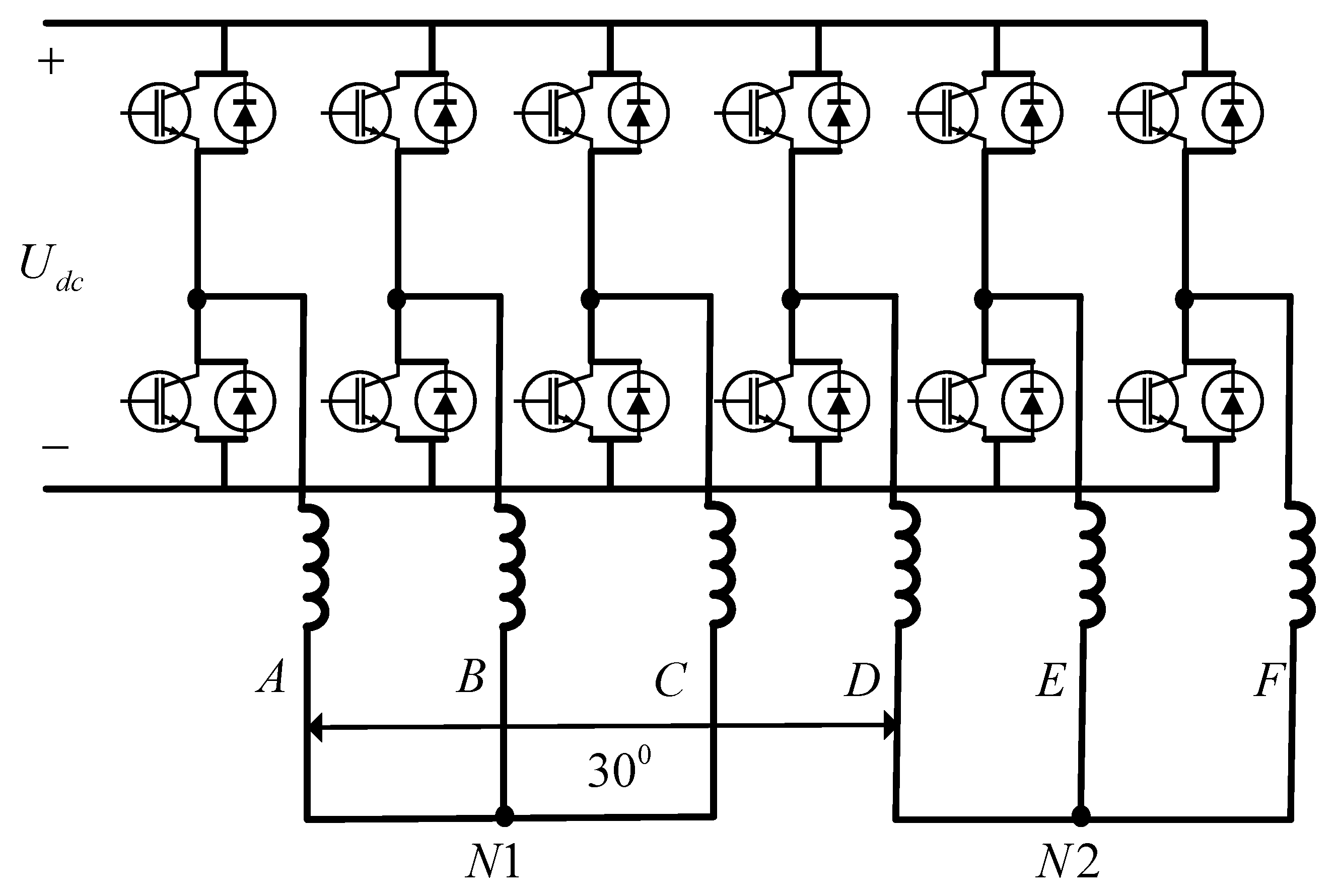
2. Mathematical Model of DT_PMSM

The driving system for DT_PMSM is shown in Figure 2. The two sets of three-phase windings are fed by two pairs of three-phase VSIs, which share the same bus voltage.

The machine model consists of three pairs of variables in mutually orthogonal subspaces based on the VSD theory. Fundamental components and harmonic components with orders of 12n ± 1 (n = 1, 2, 3…) are mapped into fundamental (α-β) subspace where electromechanical energy conversion takes place. The second (x-y) subspace represents harmonics of the order 6n ± 3, which can also be called the harmonic subspace. The third subspace is O₁-O₂ subspace where the harmonics with the order 6n ± 3 (n = 1, 3, 5…) exist, which can be omitted owing to isolated neutral points. Thus, the DT_PMSM requires current control, not only in α-β subspace but also in x-y subspace. For DT_PMSM, the amplitude invariant transform for VSD is

$$T_{VSD}=\frac{1}{3}\left[\begin{array}{cccccc}1& -\frac{1}{2}& -\frac{1}{2}& \frac{\sqrt{3}}{2}& -\frac{\sqrt{3}}{2}& 0\\ 0& -\frac{\sqrt{3}}{2}& \frac{\sqrt{3}}{2}& \frac{1}{2}& \frac{1}{2}& -1\\ 1& -\frac{1}{2}& -\frac{1}{2}& -\frac{\sqrt{3}}{2}& \frac{\sqrt{3}}{2}& 0\\ 0& -\frac{\sqrt{3}}{2}& \frac{\sqrt{3}}{2}& \frac{1}{2}& \frac{1}{2}& -1\end{array}\right]$$

(1)

The variables in fundamental subspace are transformed into a rotor coordinate system in order to achieve vector control. The expression of the rotational transformation is

$$T_{dq}=\left[\begin{array}{cccccc}\cos \theta & \sin \theta & 0& 0& 0& 0\\ -\sin \theta & \cos \theta & 0& 0& 0& 0\\ 0& 0& 1& 0& 0& 0\\ 0& 0& 0& 1& 0& 0\end{array}\right]$$

(2)

On the condition that the back electromotive force (EMF) is sinusoidal, saturation and mutual leakage inductance are ignored, and two sets of three-phase windings are identical. The two sets of voltage equations after the rotational transformation (Equation (2)) can be expressed as follows.

$$\{\begin{array}{c}{u}_d=i_{d}R+L_d\frac{d{i}_d}{dt}-w_e{L}_q{i}_q\\ u_q=i_{q}R+L_q\frac{d{i}_q}{dt}+w_e(L_d{i}_d+{\psi }_f)\\ u_x=i_{x}R+L_z\frac{d{i}_x}{dt}\\ u_y=i_{y}R+L_z\frac{d{i}_y}{dt}\end{array}$$

(3)

where R is the stator resistance, L_d and L_q represent the d- and q-axes inductances, respectively, L_z is stator self leakage inductance. The electrical angular speed is represented by w_e, and ψ_f denotes the permanent magnet flux.

3. Current Regulator Design in Fundamental Subspace

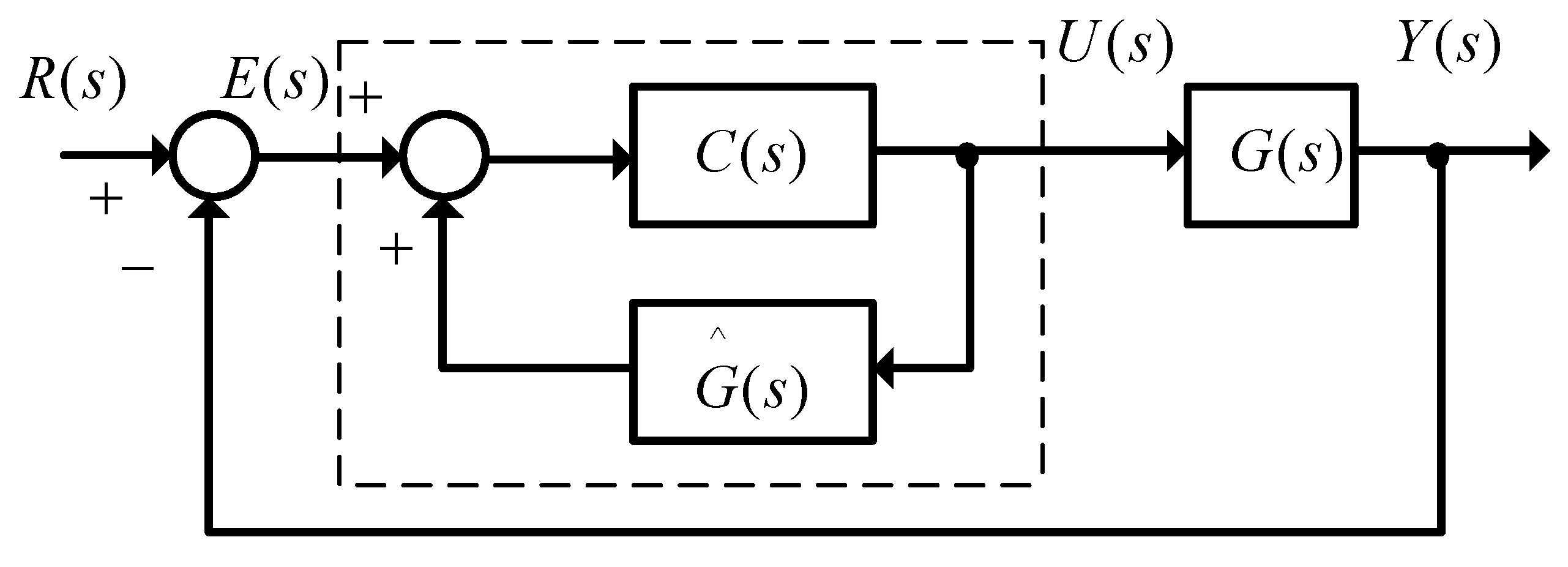
3.1. Traditional IMC Method

Figure 3 illustrates the block diagram of the traditional IMC method, which uses internal model $\hat{G}$(s) in parallel with the controlled plant G(s) and the control loop is augmented with an internal current controller C(s).

Supposing that the internal model is perfect, i.e., $\hat{G}$(s) = G(s) and the transfer function for the system can be expressed as

$$G_c(s)=C(s)G(s)$$

(4)

F(s) is the controller which represents the dotted line part and can be expressed as

$$F(s)=\frac{U(s)}{E(s)}=\frac{C(s)}{I-C(s)\widehat{G}(s)}$$

(5)

In terms of the theory of IMC [6,9], C(s) can be tuned with a low-pass filter as shown in Equation (6).

$$C(s)={\widehat{G}}^{-1}(s)L(s)=G^{-1}(s)L(s)$$

(6)

where L(s) is defined as in Equation (7).

$$L(s)=\frac{1}{\lambda s+1}$$

(7)

where λ is the time constant and L(s) is a low pass filter.

According to Equations (5)–(7), the current controller is acquired as follows.

$$F(s)=\frac{1}{\lambda }\left[\begin{array}{cc}{L}_d(1+\frac{R}{s{L}_d})& 0\\ 0& L_q(1+\frac{R}{s{L}_q})\end{array}\right]$$

(8)

The closed-loop transfer function is derived as follows.

$$G_c(s)=\frac{1}{\lambda s+1}I$$

(9)

From the above analysis, it is obvious that IMC gives the explicit physical meaning of the time constant for the low pass filter. Besides, the explicit expressions of proportional and integral are determined. The response speed for the control system is closely associated with λ. As λ decreases, the response speed gets faster.

Figure 4 illustrates the block diagram of current regulator design based on the IMC.

For nominal motor parameters, the real currents (i_d and i_q) will be identical to the model currents i_d^sim and i_q^sim.

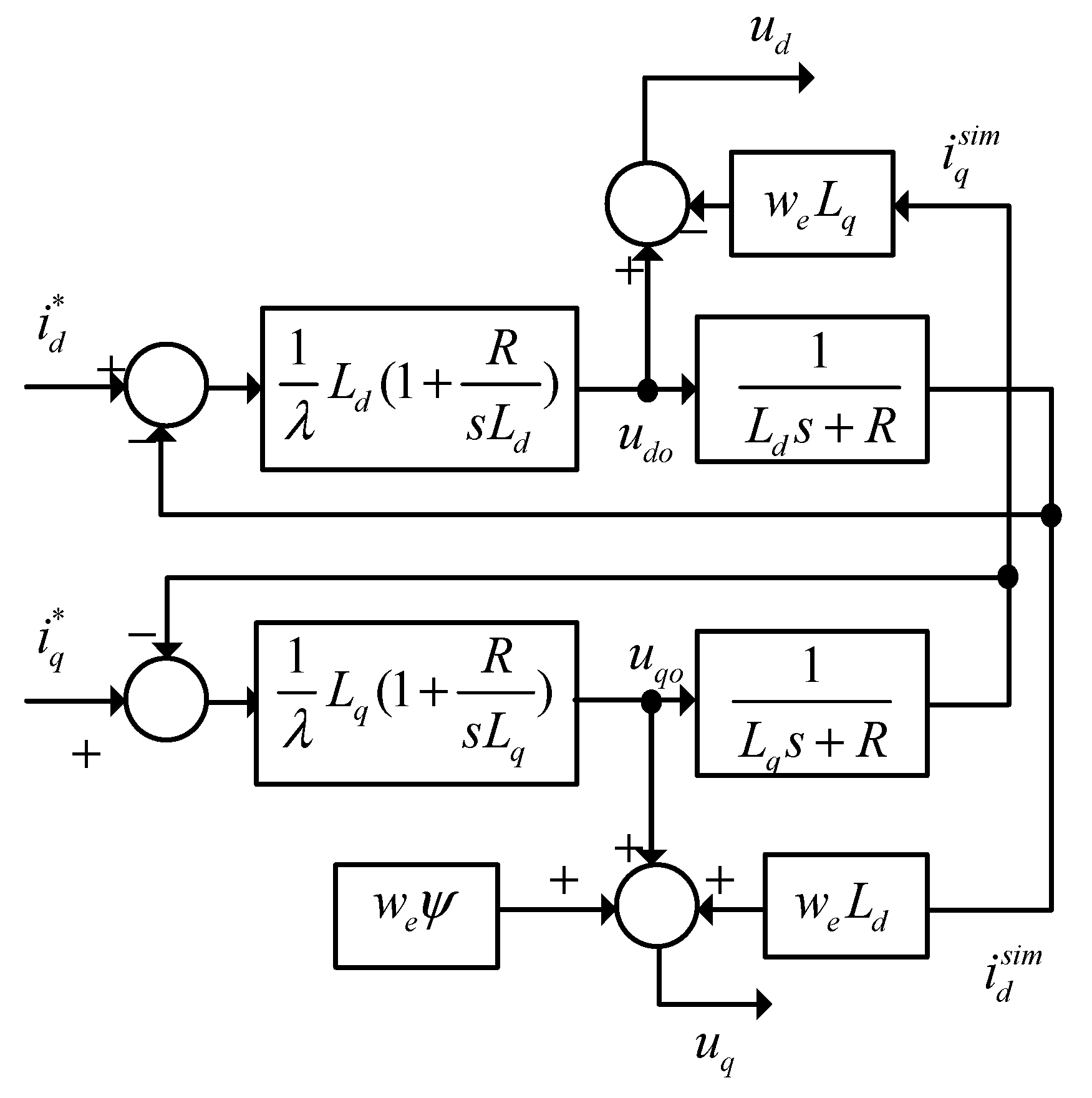
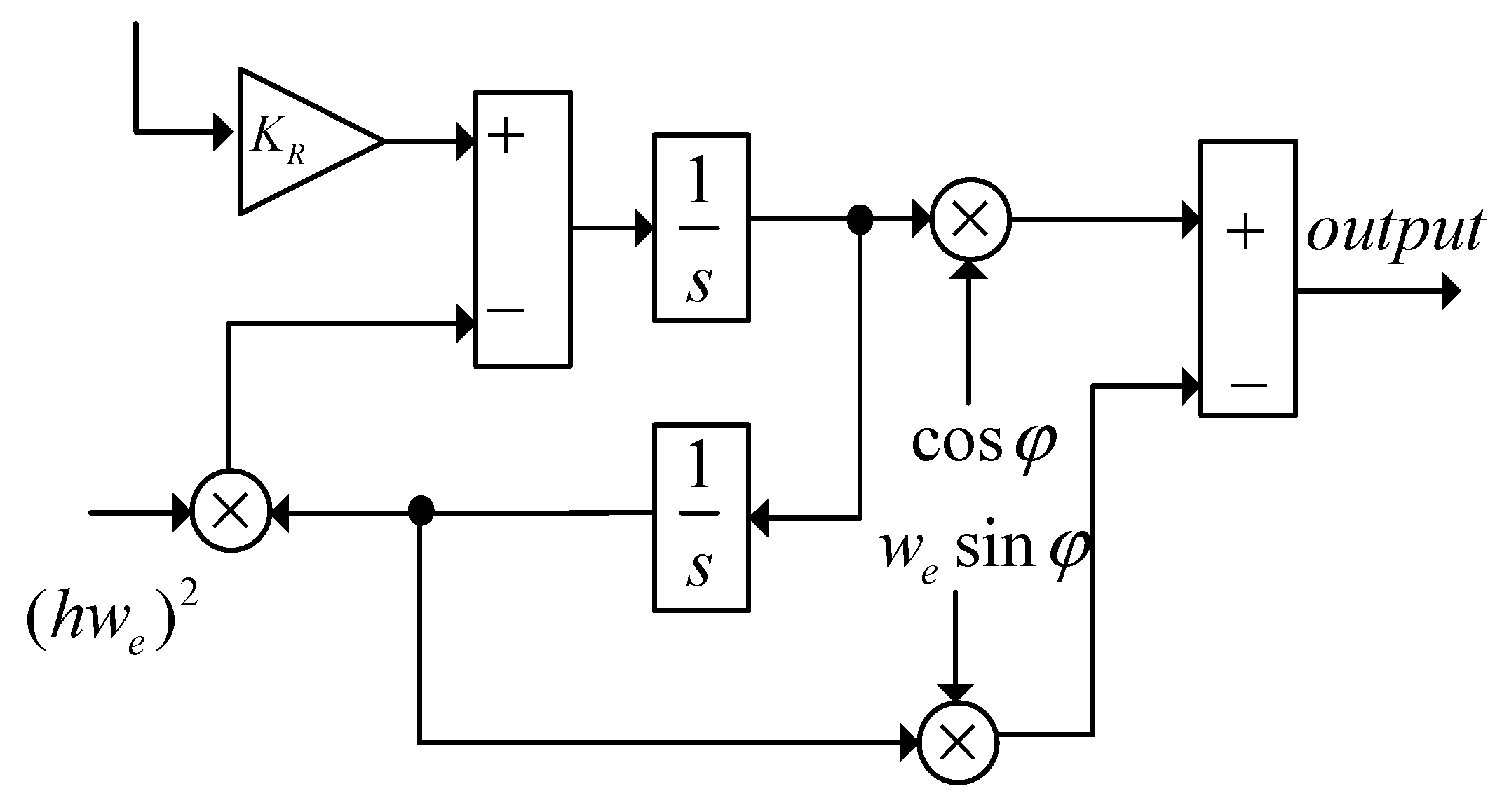
3.2. Sliding Mode Control Based on the Internal Model

In practice, the system is affected by parameter perturbation, external disturbance and other factors, so the voltage equations in α-β subspace shown in Equation (3) can be rewritten as follows.

$$\{\begin{array}{l}{u}_d=R{i}_d+L_d\frac{d{i}_d}{dt}-w_e{L}_q{i}_q+h_d(x,t)\\ u_q=R{i}_q+L_q\frac{d{i}_q}{dt}+w_e{L}_d{i}_d+w_e{\psi }_f+h_d(x,t)\\ h_d(x,t)={\epsilon }_d+{\zeta }_d=\mathsf{\Delta }R{i}_d+\mathsf{\Delta }{L}_d\frac{d{i}_d}{dt}-\mathsf{\Delta }{L}_q{i}_q{w}_e+{\zeta }_d\\ h_q(x,t)={\epsilon }_q+{\zeta }_q=\mathsf{\Delta }R{i}_q+\mathsf{\Delta }{L}_q\frac{d{i}_q}{dt}+\mathsf{\Delta }{L}_d{i}_d{w}_e+\mathsf{\Delta }{\psi }_f{w}_e+{\zeta }_q\end{array}$$

(10)

where ΔL_d, ΔL_q, ΔR and Δψ_f are the variations of L_d, L_q, R and ψ_f, respectively; ε_d and ε_q represent the uncertainties caused by the parameter variations, which can be DC components. While ζ_d and ζ_q are the equivalents of external disturbances and un-modeled parts.

The objective of robust current control is to find a suitable control law u₁, which can eliminate the disturbance h (x, t). So u₁ can be expressed as follows

$$u_1=h(x,t)$$

(11)

In order to improve the performance of IMC strategy shown in Figure 4 and enhance the robustness of the system, sliding mode control (SMC) strategy is introduced to make the output meet the requirements of Equation (12). Since the system has robustness to disturbance only in the sliding mode stage, in order to ensure the robustness of the system, it is necessary to make the system work in the sliding mode stage as far as possible in the whole motion process. Therefore, the sliding mode surface for d-axis current is defined as

$$\{\begin{array}{l}{S}_d=i_d+Z_d\\ \frac{d{Z}_d}{dt}=\frac{R{i}_d-u_{d0}}{L_d}\\ Z_d(0)=0\end{array}$$

(12)

where u_d0 is the output voltage of IMC in d-axis.

The sliding surface ensures that the state trajectory of the system is on the sliding surface at the beginning, which can avoid the approaching motion and ensure the robustness of the system in the whole motion process.

According to Equations (3) and (12) and substituting i_q^sim to i_q, the derivation of sliding mode surface for time t is

$$\frac{d{S}_d}{dt}=\frac{w_e{L}_q{i}_q+u_d-u_{d0}}{L_d}$$

(13)

The Lyapunov function candidate is given by

$$V_d(t)=\frac{1}{2}{S}_d^2(t)$$

(14)

The time derivative of Equation (14) is derived as follows.

$$\frac{d{V}_d(t)}{dt}=S_d(t)\frac{d{S}_d(t)}{dt}$$

(15)

In order to ensure the stability of the system, $\frac{{dV}_d\left(t\right)}{dt}\le 0$ should be satisfied according to Lyapunov stability theory. Therefore, the sliding mode control law for the d-axis current is defined as

$$\{\begin{array}{l}{u}_d=L_d(-a\left|x_d\right|\mathrm{sgn}(S_d)-b{S}_d)+u_{d0}-w_e{L}_q{i}_q^{sim}\\ x_d=i_d^{*}-i_d\end{array}$$

(16)

According to Equations (13), (15) and (16), $\frac{{dV}_d\left(t\right)}{dt}$ can be acquired as follows.

$$\frac{d{V}_d(t)}{dt}=S_d(-a\left|x_d\right|\mathrm{sgn}(S_d)-b{S}_d)$$

(17)

$\frac{{dV}_d\left(t\right)}{dt}\le 0$ can be guaranteed when a $>0$ and b $>0$. The existence and accessibility of the d-axis current sliding mode can be guaranteed, i.e., the system can realize the sliding mode motion, so the d-axis current sliding mode control system is stable.

Similarly, the current sliding surface for q-axis is

$$\{\begin{array}{l}{S}_q=i_q+Z_q\\ \frac{d{Z}_q}{dt}=\frac{R{i}_q-u_{q0}}{L_q}\\ Z_q(0)=0\end{array}$$

(18)

The q-axis current sliding mode control law can be defined as follows.

$$\{\begin{array}{l}{u}_q=L_q(-a\left|x_q\right|\mathrm{sgn}(S_q)-b{S}_q)+u_{q0}+w_e(L_d{i}_d^{sim}+\psi )\\ x_q=i_q^{*}-i_q\end{array}$$

(19)

In order to suppress the chattering of sliding mode, the symbolic functions in Equation (20) are used instead of the symbolic functions in Equations (16) and (19).

$$sat(S)=\{\begin{array}{ll}1,& S>1\\ S,& \left|S\right|<1\\ -1,& S<-1\end{array}$$

(20)

where S can represent S_d and S_q.

The block diagram of sliding mode control based on the internal model is shown in Figure 5.

Take d-axis as an example to prove robustness. The switching function will be affected by the factors such as parameter perturbation and external disturbance. Equation (21) can be redefined as

$$\frac{d{S}_d(t)}{dt}=\frac{u_d+w_e{L}_q{i}_q^{sim}-u_{d0}}{L_d}-\frac{h_d}{L_d}$$

(21)

According to Equations (16), (17) and (21), the term $\frac{{dV}_d\left(t\right)}{dt}$ is given by

$$\frac{d{V}_d(t)}{dt}=S_d(-a\left|x_d\right|sat(S_d)-\frac{h_d}{L_d})-b{S}_d^2$$

(22)

$\frac{d{V}_d\left(t\right)}{dt}\le 0$ can be guaranteed when a$\left|x_d\right|$L_d > $\left|h_d\right|$. The robustness of the whole system is proved by guaranteeing that the sliding mode of the system is invariant to the motor parameters and external disturbances.

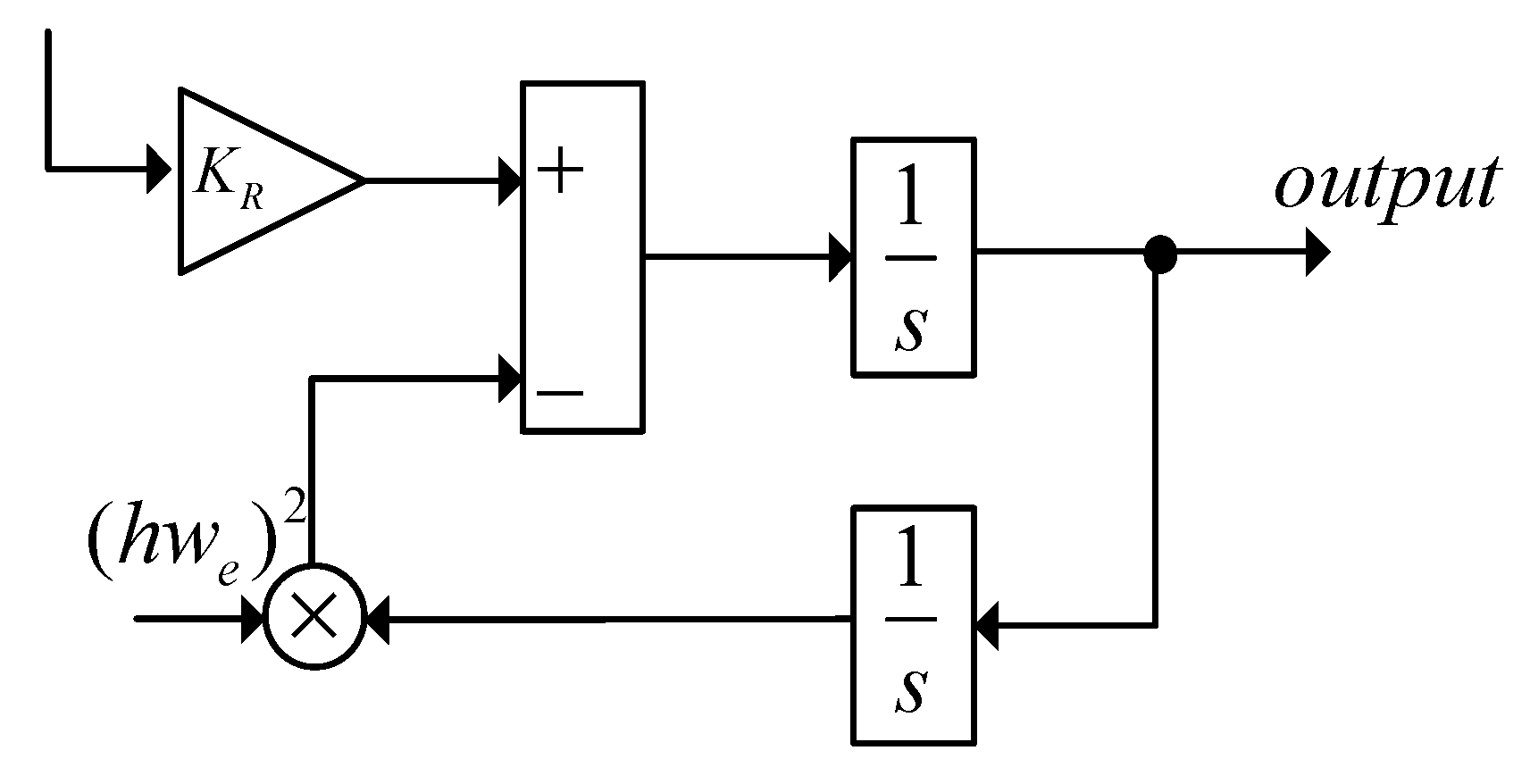
4. Current Regulator Design in Harmonic Subspace

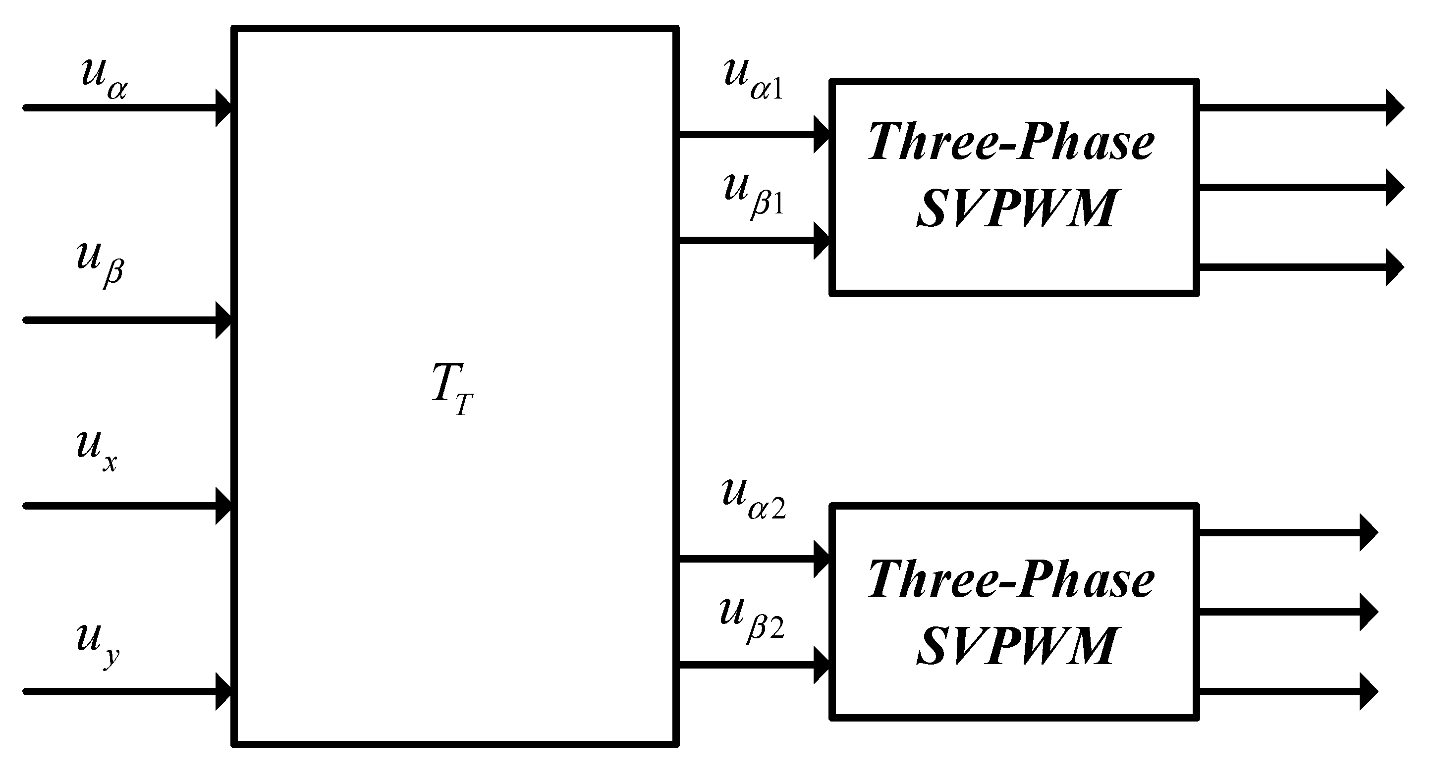
Based on the VSD theory [6,7], the currents in both subspaces can be expressed as follows.

$$\overrightarrow{i_{\alpha \beta }}=i_{\alpha }+j{i}_{\beta }=i_{\alpha 1}+i_{\alpha 2}+j(i_{\beta 1}+i_{\beta 2})$$

(23)

$$\overrightarrow{i_{xy}}=i_x+j{i}_y=i_{\alpha 1}-i_{\alpha 2}-j(i_{\beta 1}-i_{\beta 2})$$

(24)

The fifth and seventh harmonic currents in two sets of three-phase windings can be expressed as follows.

$$\{\begin{array}{l}{\overrightarrow{I}}_{\alpha \beta 1}^h=k_{1}I{e}^{-5j{w}_{e}t}+k_{2}I{e}^{7j{w}_{e}t}\\ {\overrightarrow{I}}_{\alpha \beta 2}^h=k_{3}I{e}^{-5j{w}_{e}t}+k_{4}I{e}^{7j{w}_{e}t}\end{array}$$

(25)

where the weights of fifth and seventh harmonic currents for windings ABC are represented by k₁ and k₂, and k₃ and k₄ denote the weights of fifth and seventh harmonic currents in the other windings.

In terms of Equation (1), the harmonic currents in harmonic subspaces are expressed as

$${\overrightarrow{I}}_{xy}^h=(k_1-k_3)I{e}^{5j{w}_{e}t}+(k_2-k_4)I{e}^{-7j{w}_{e}t}$$

(26)

In order to transform the +5w_e and −7w_e harmonic currents to +6w_e and −6w_e, respectively, a new synchronous rotating coordinate transformation is suggested as in Equation (27).

$$T_T=\left[\begin{array}{cccccc}\cos \theta & \sin \theta & 0& 0& 0& 0\\ -\sin \theta & \cos \theta & 0& 0& 0& 0\\ 0& 0& \cos \theta & -\sin \theta & 0& 0\\ 0& 0& \sin \theta & \cos \theta & 0& 0\end{array}\right]$$

(27)

By applying the transformation T_T, the sixth harmonic currents can be given by

$$\left[\begin{array}{c}{I}_{x1}^6\\ I_{y1}^6\end{array}\right]=\left[\begin{array}{c}{I}_{xs}\sin (6w_{e}t)+I_{xc}\cos (6w_{e}t)\\ I_{ys}\sin (6w_{e}t)+I_{yc}\cos (6w_{e}t)\end{array}\right]$$

(28)

Resonant controller can follow the tracks of sinusoidal references with zero steady-state error, which is a perfect substitute to traditional proportional-integral (PI) controllers designed in both positive-sequence and negative-sequence synchronous reference frames (SRF) simultaneously [19,20]. Besides this, it has the merits of a low computational burden because it lacks in multiple coordinate transformations compared to traditional PI controllers. Therefore, it is appropriate for the current harmonic suppression.

The suggested resonant controller which can follow the track of harmonic of order h is expressed in s-domain as follows.

$$G_R(s)=K_R\frac{s}{s^2+{(h{w}_e)}^2}$$

(29)

where w_e is the fundamental frequency, h is the harmonic order, K_R is the resonant gain.

As proposed by A. G. Yepes in [19], the transfer function can be decomposed in a scheme with two integrators, as depicted in Figure 6, which is widely employed because it has the merits of discretizing the integrators separately and can adjust the frequency according to the operating frequency of motor.

Owing to the inductive load (leakage inductance L_z and resistance R) in x-y subspace, the control delay and PWM update delay, there will be a phase delay which varies with the operating frequency and the PWM control period. So phase compensation is essential to ensure the stability of resonant controller. The resonant controller with phase compensation, as shown in Figure 7, can be rewritten in the s-domain as follows.

$$G_R^C(s)=K_R\frac{s\cos \phi -h{w}_e\sin \phi }{s^2+{(h{w}_e)}^2}$$

(30)

where $\phi$ is the compensating angle.

Phase leading angle is supposed to be calculated in order to guarantee the stability of current regulator in harmonic subspace. In order to demonstrate the influences of PWM, a ZOH model in x-y subspace that contains one switching period delay owing to PWM update delay and computation delay is given by

$$P(z)=\frac{z^{-2}}{R}\frac{1-e^{-R{T}_S/L_Z}}{1-z^{-1}{e}^{-R{T}_S/L_Z}}$$

(31)

It is noteworthy that L_Z and R denote leakage inductance and resistance in harmonic subspace, respectively. Equation (32) is supposed to be satisfied for the purpose of making compensations for the phase delay.

$$\phi =-\angle P(z)=-\arctan (\frac{e^{-R{T}_S/L_z}\sin (h{w}_e{T}_s)-\sin (2h{w}_e{T}_s)}{\cos (2h{w}_e{T}_s)-e^{-R{T}_S/L_z}\cos (h{w}_e{T}_s)})$$

(32)

λ is defined as the slope of $-\angle P(z)$ at frequency hw_e.

$$\lambda =-\frac{\partial \angle P(z)}{\partial (h{w}_e)}=T_s\frac{2+e^{-2R{T}_s/L_z}-3e^{-R{T}_s/L_z}\cos (h{w}_e{T}_s)}{1+e^{-2R{T}_s/L_z}-2e^{-R{T}_s/L_z}\cos (h{w}_e{T}_s)}$$

(33)

Equation (34) can be derived based on the assumption that T_s is small.

$$e^{-2R{T}_s/L_z}\approx 1-\frac{2R{T}_s}{L_z}\approx 1, e^{-R{T}_s/L_z}\approx 1-\frac{R{T}_s}{L_z}\approx 1$$

(34)

According to Equations (32)–(34), λ can be calculated, which is approximately 1.5. If w_e is equal to 0, $\phi$ is 0. Therefore, $\phi$ is approximately calculated as in Equation (35).

$$\phi =1.5h{w}_e{T}_s$$

(35)

5. PWM Strategy

Based on the VSD theory, the voltage vectors in the fundamental and harmonic subspaces are required to be modulated at the same time. By regarding the six-phase VSI as two sets of three-phase VSIs with 30 degrees phase shift, the voltage vectors for two independent three-phase VSIs are expressed as

$$\overrightarrow{u_{\alpha \beta 1}}=u_{a1}+j{u}_{\beta 1}\overrightarrow{u_{\alpha \beta 2}}=u_{a2}+j{u}_{\beta 2}$$

(36)

where $\overrightarrow{u_{\alpha \beta 1}}$ and $\overrightarrow{u_{\alpha \beta 2}}$ are the voltage vectors of two three-phase windings, respectively. The α-β voltage components in ABC phase windings can be represented by $u_{\alpha 1}$ and $u_{\beta 1}$. While $u_{\alpha 2}$ and $u_{\beta 2}$ can denote the α-β voltage components in the other phase winding.

The expressions for the reference voltage vectors in the fundamental and harmonic subspaces are given in Equations (37) and (38), respectively.

$$\overrightarrow{u_{\alpha \beta }}=u_{\alpha }+j{u}_{\beta }=u_{\alpha 1}+u_{\alpha 2}+j(u_{\beta 1}+u_{\beta 2})$$

(37)

$$\overrightarrow{u_{xy}}=u_x+j{u}_y=u_{\alpha 1}-u_{\alpha 2}-j(u_{\beta 1}-u_{\beta 2})$$

(38)

where $\overrightarrow{u_{\alpha \beta }}$ and $\overrightarrow{u_{xy}}$ are the voltage vectors in fundamental and harmonic subspaces, respectively. It is noteworthy that the x-y components take inverted signs.

According to Equations (37) and (38), the voltage vectors of six-phase VSI can be expressed by the voltage vectors of two sets of three-phase VSI, as illustrated in Equation (39).

$$\overrightarrow{u_{\alpha \beta 1}}=\overrightarrow{u_{\alpha \beta }}+\overrightarrow{u_{xy}^{\ast }} \overrightarrow{u_{\alpha \beta 2}}=e^{-j{30}^0}(\overrightarrow{u_{\alpha \beta }}-\overrightarrow{u_{xy}^{\ast }})$$

(39)

where $\overrightarrow{u_{xy}^{*}}$ is the conjugate function of $\overrightarrow{u_{xy}}$.

The expression of Equation (39) in the matrix form can be found in Equation (40).

$${\left[\begin{array}{cccc}{u}_{\alpha 1}& u_{\beta 1}& u_{\alpha 2}& u_{\beta 2}\end{array}\right]}^T=T_T{\left[\begin{array}{cccc}{u}_{\alpha }& u_{\beta }& u_x& u_y\end{array}\right]}^T$$

(40)

where T_T is

$$T_T=\left[\begin{array}{cccc}1& 0& 1& 0\\ 0& 1& 0& -1\\ \frac{\sqrt{3}}{2}& \frac{1}{2}& -\frac{\sqrt{3}}{2}& \frac{1}{2}\\ -\frac{1}{2}& \frac{\sqrt{3}}{2}& \frac{1}{2}& \frac{\sqrt{3}}{2}\end{array}\right]$$

(41)

The traditional three-phase SVPWM algorithm can be used to modulate the reference voltage vectors in the fundamental and harmonic subspace at the same time according to Equations (40) and (41). Figure 8 illustrates the PWM strategy for DT_PMSM.

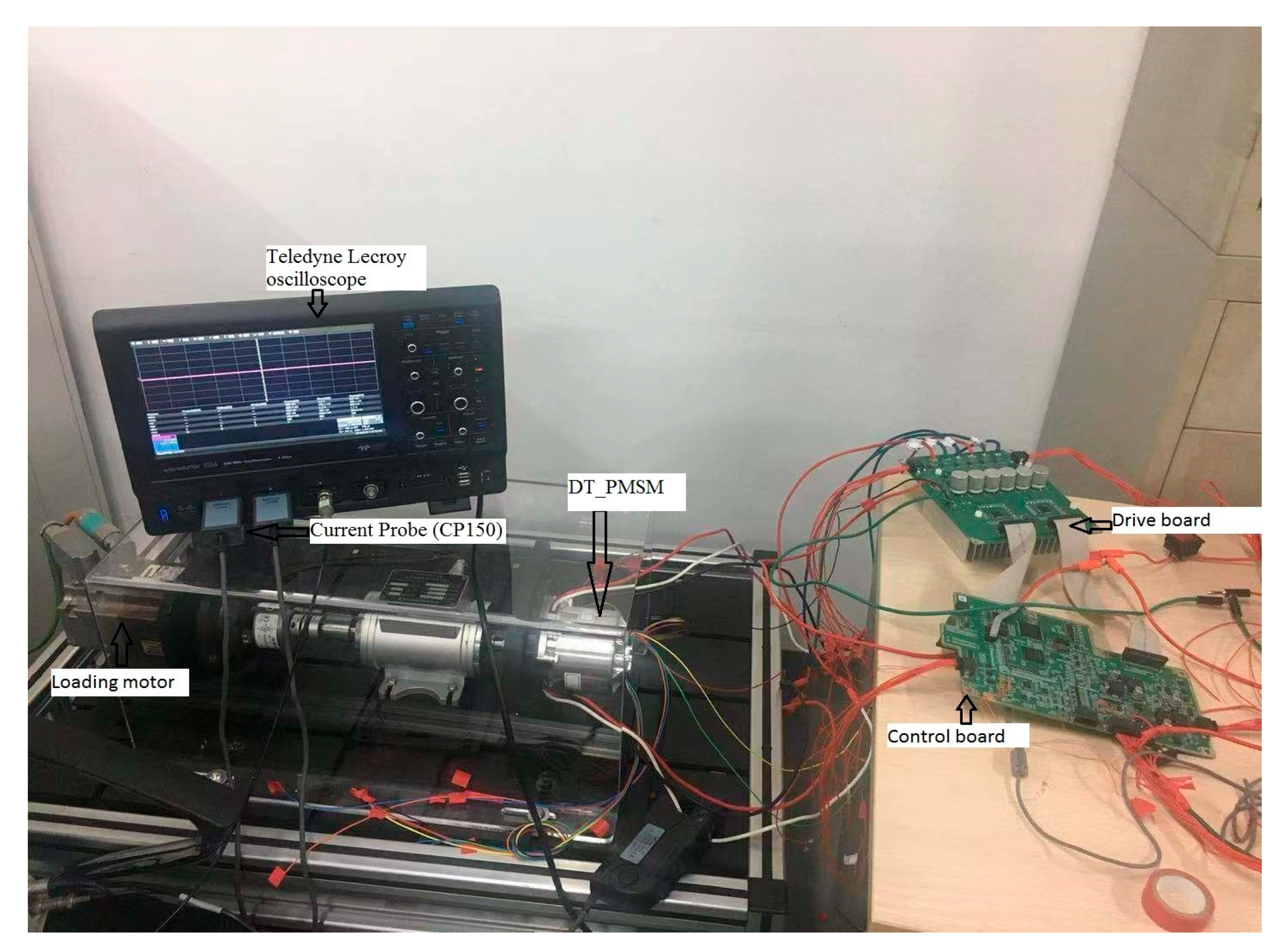
6. Experimental Verification

The proposed control algorithm is illustrated in Figure 9, which includes current regulators in both α-β and x-y subspaces.

Figure 10 shows the experimental platform of DT_PMSM where the performance of the suggested control algorithm is verified. It consists of a DT_PMSM, a brushless direct current motor (BLDC) dynamometer, a drive board and a control board. The BLDC dynamometer operating in the speed-control mode or load torque mode can be used as a loading machine. The DT_PMSM is fed by a two-level VSI, which is connected to 12 V DC bus voltage. The PWM cycle is 50 μs and the dead time is set to be 1 μs. The control actions are performed by an Aurix TC277 DSP which provides 12 PWMs.

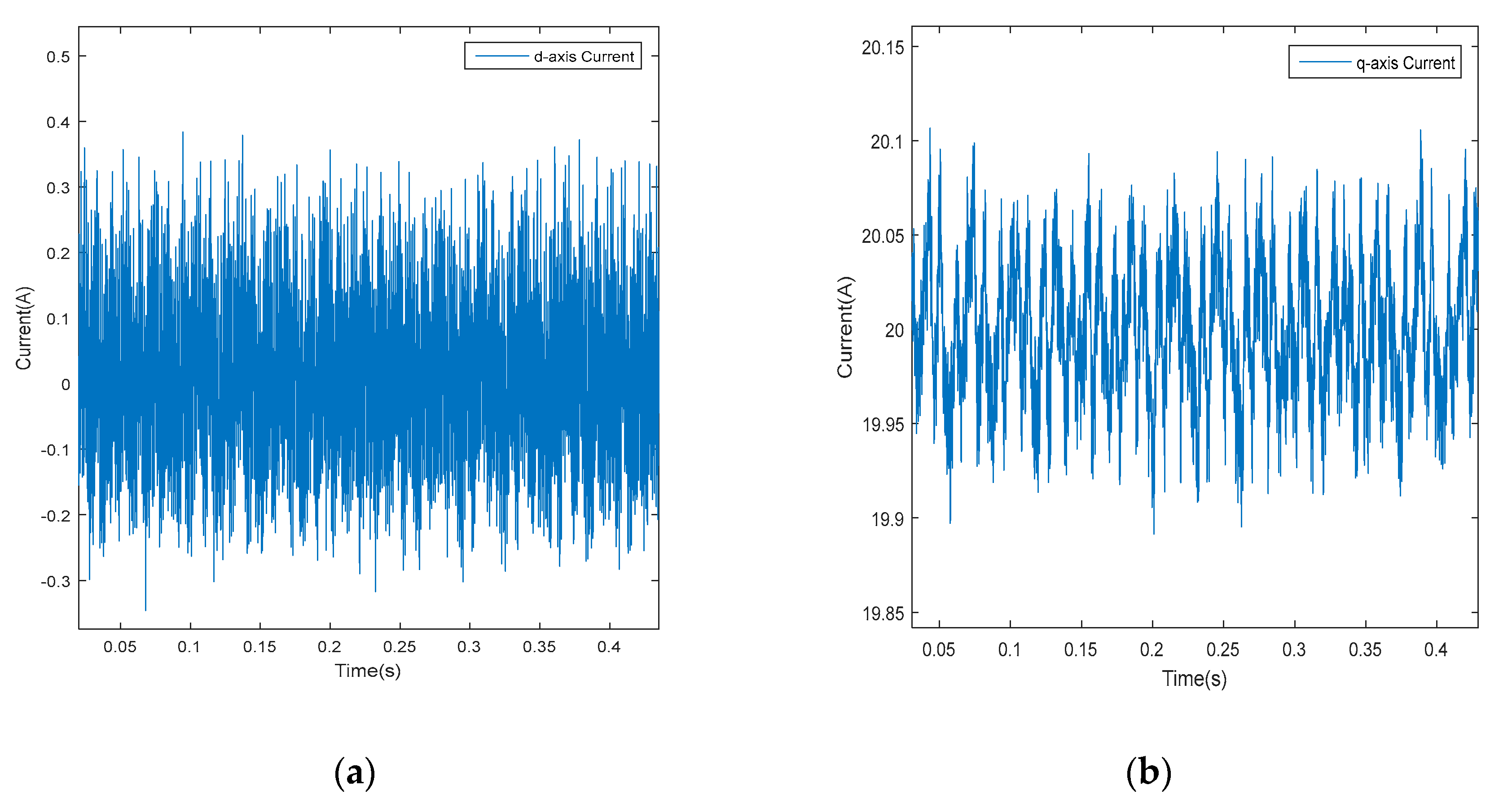
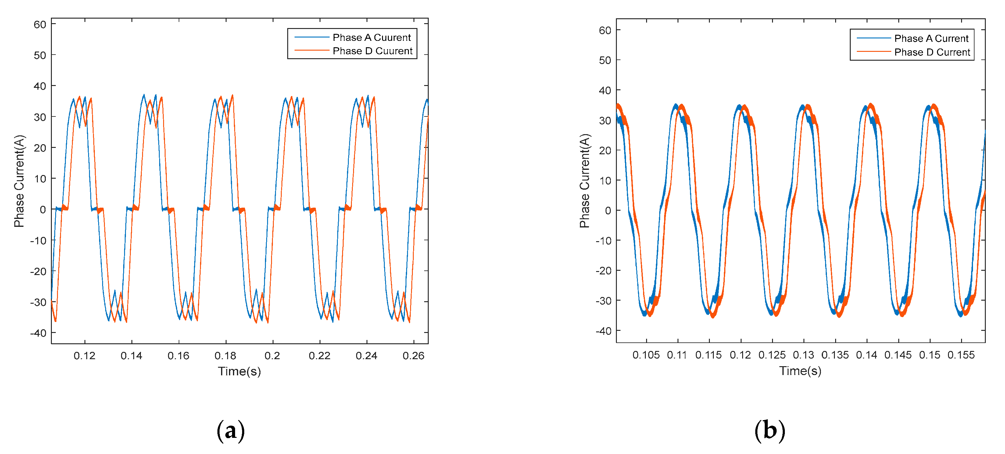
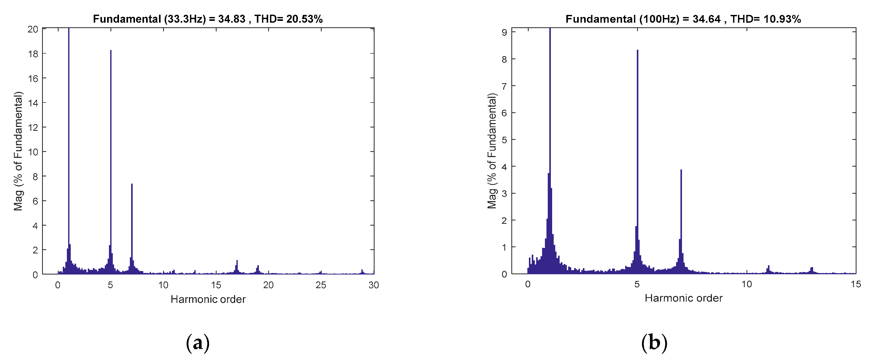
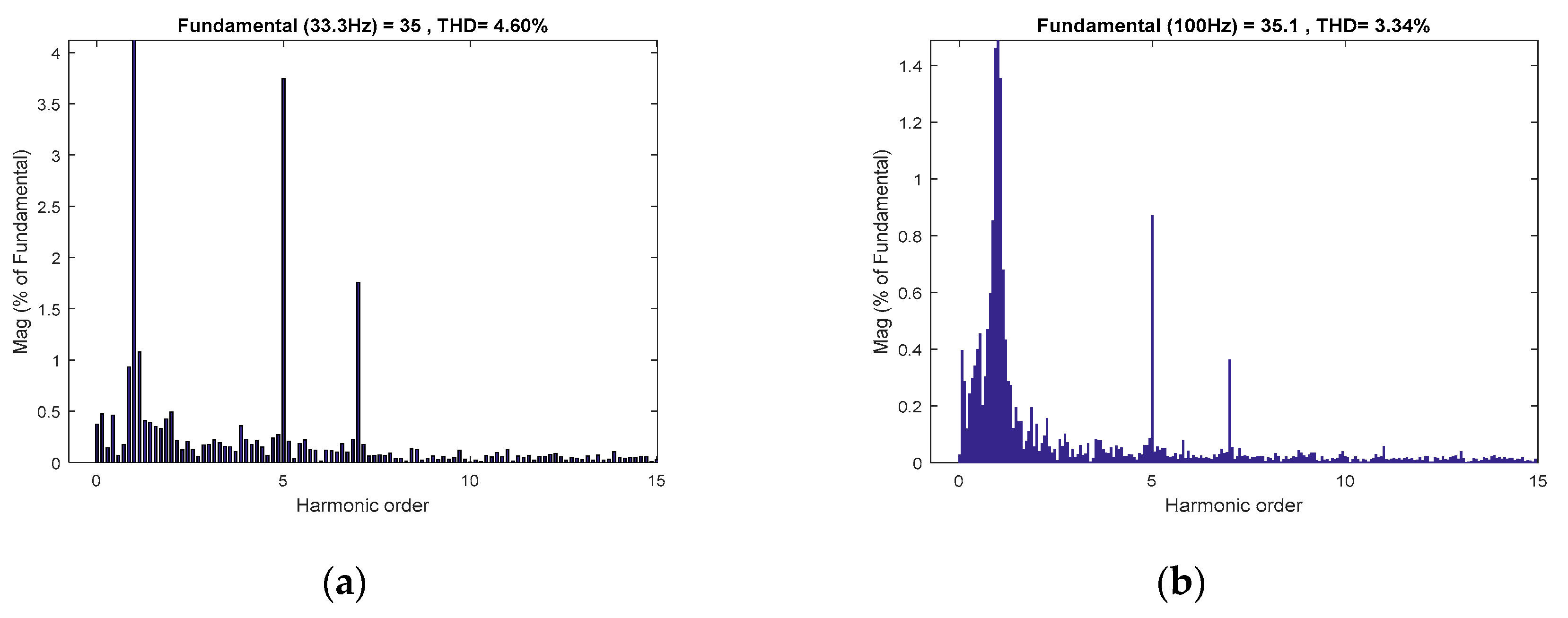
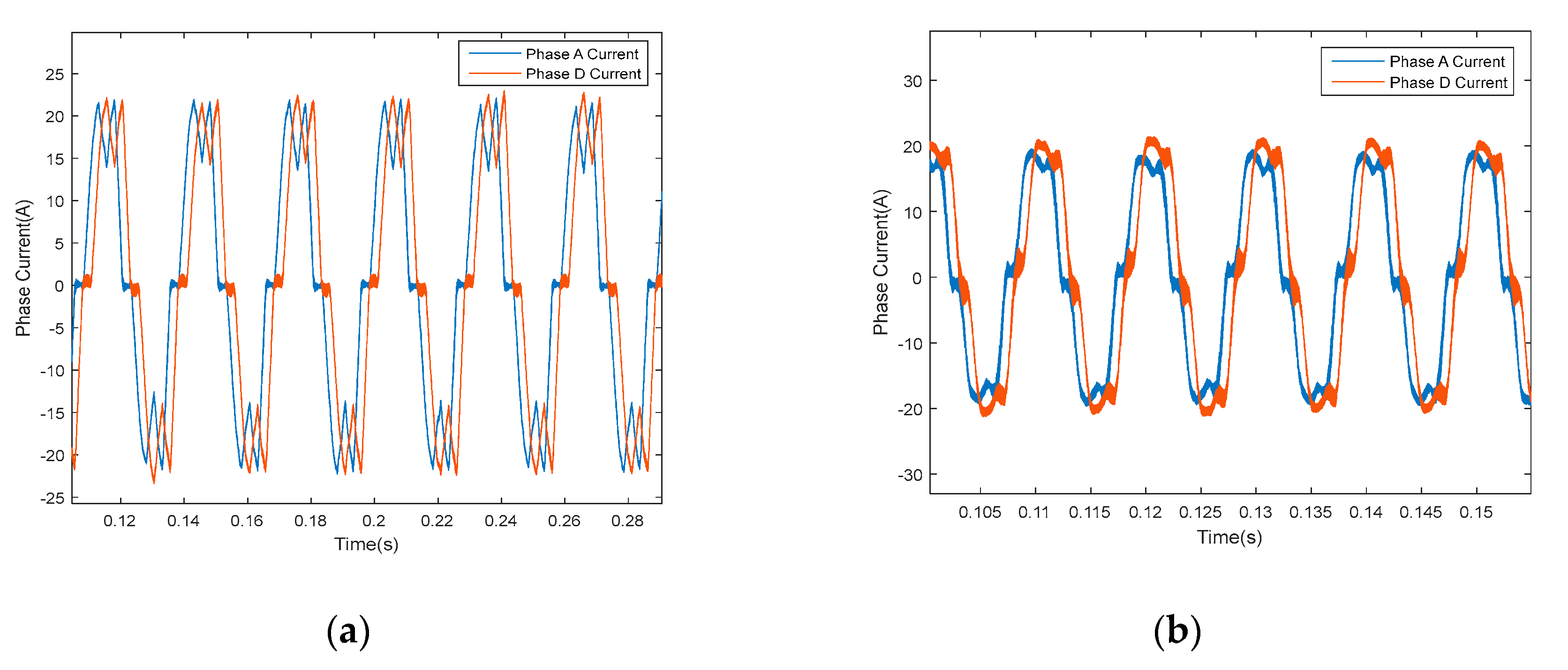
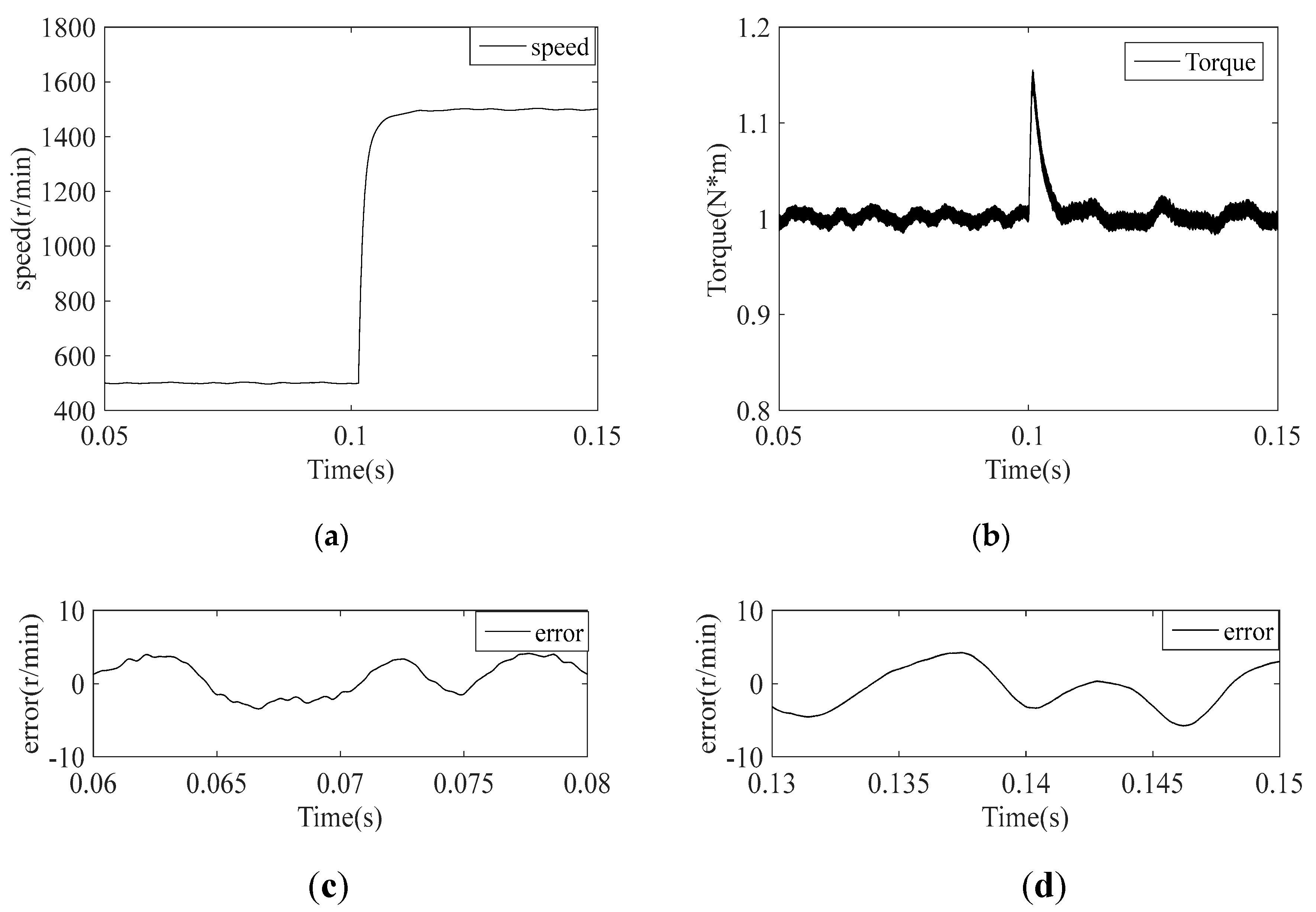
6.1. Traditional IMC Method

The reference currents of d- and q-axes are 0 A and 20 A. In fundamental subspace, the current regulator is designed on the basis of the system uncertainties R’ = 0.7R, L_d’ = 0.5L_d, L_q’ = 0.7L_q, ψ_f’ = 0.8ψ_f and the un-modelled dynamics of d- and q-axes are unknown, which can validate the robustness against uncertainty capability.

Table 1. Motor parameters.

Parameter	Value
d-axis inductance	0.08 mH
q-axis inductance	0.08 mH
Leakage inductance	0.0072 mH
Permanent Magnet Flux	0.005 Wb
Stator Resistance	0.0113 Ω
Pole Pairs	4
Rated Power	500 W
DC Bus Voltage	12 V

gives the parameters of DT_PMSM. The experimental results of the proposed scheme are compared to the traditional internal model control without sliding mode control. In both schemes, λ is chosen to be 0.005.

Figure 11 illustrates the d- and q-axes current performances using the traditional IMC method. One can see that the real currents of d- and q-axes fluctuate around the set current values. Because the traditional PI controller cannot track and adjust the AC quantity without static steady error due to its limited bandwidth, although it can compensate the voltage error caused by the resistance disturbance, inductance disturbance and flux disturbance, which are DC disturbance components.

Figure 12 depicts the d- and q-axes current performances after adopting the proposed current control algorithm. It is clearly shown that the currents, after using the proposed method, are smoother with smaller fluctuations than those found in the conventional method. So the proposed control scheme in α-β subspace can achieve better current control performance.

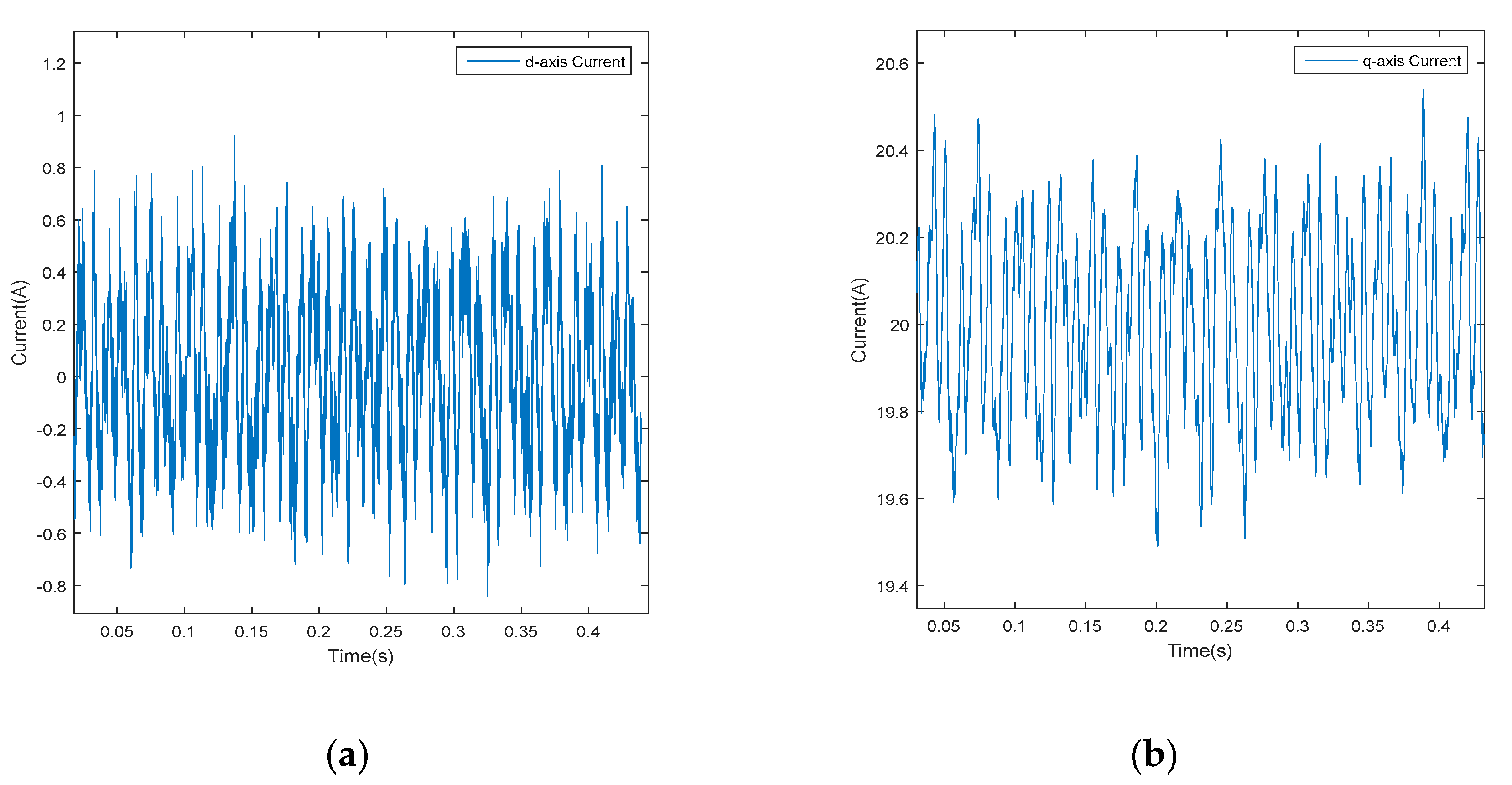
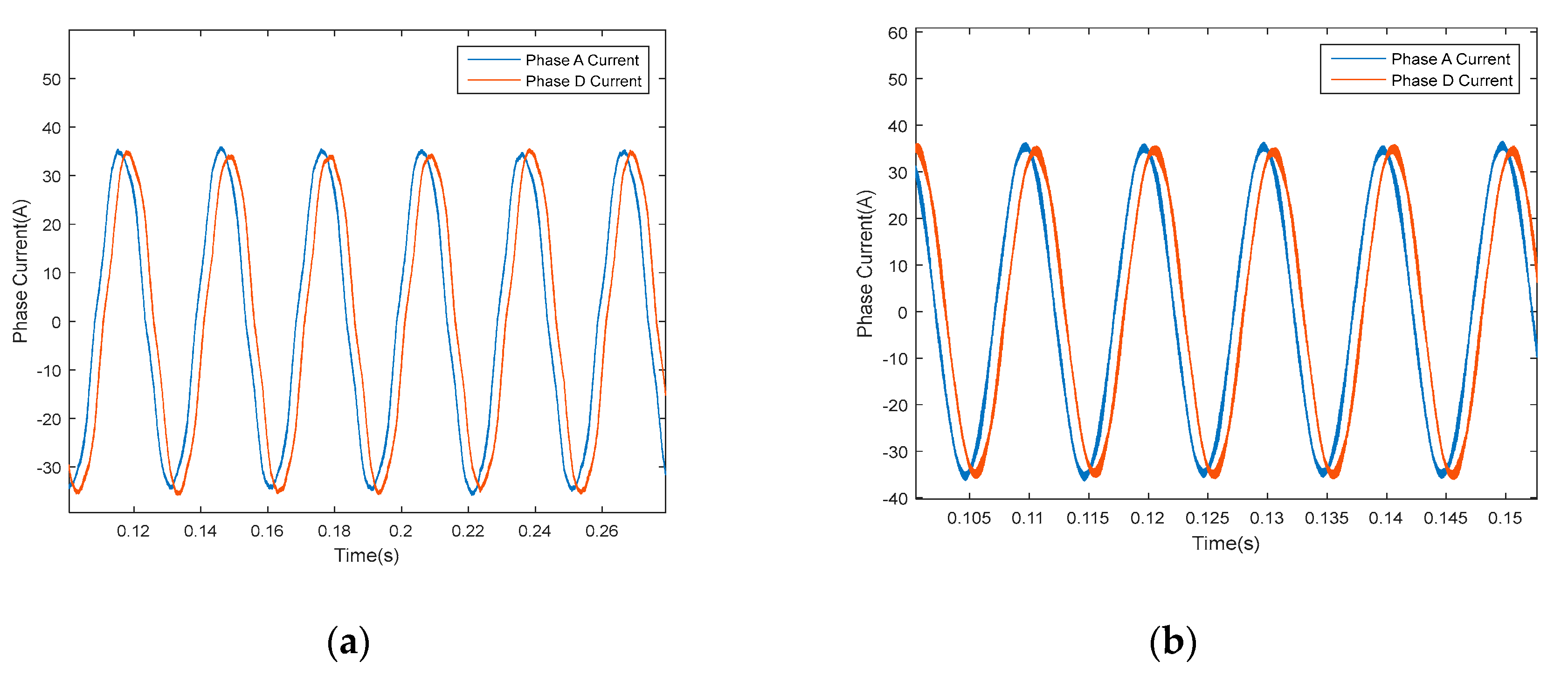
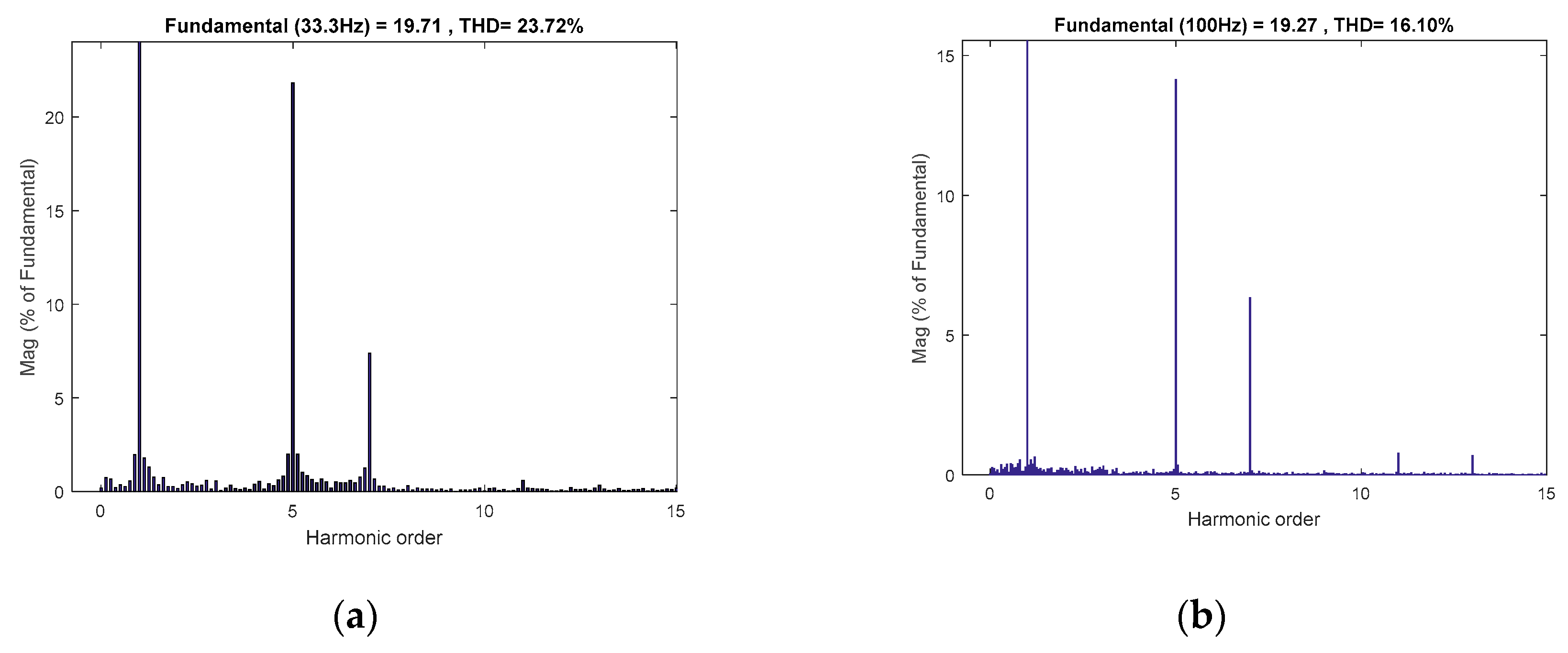
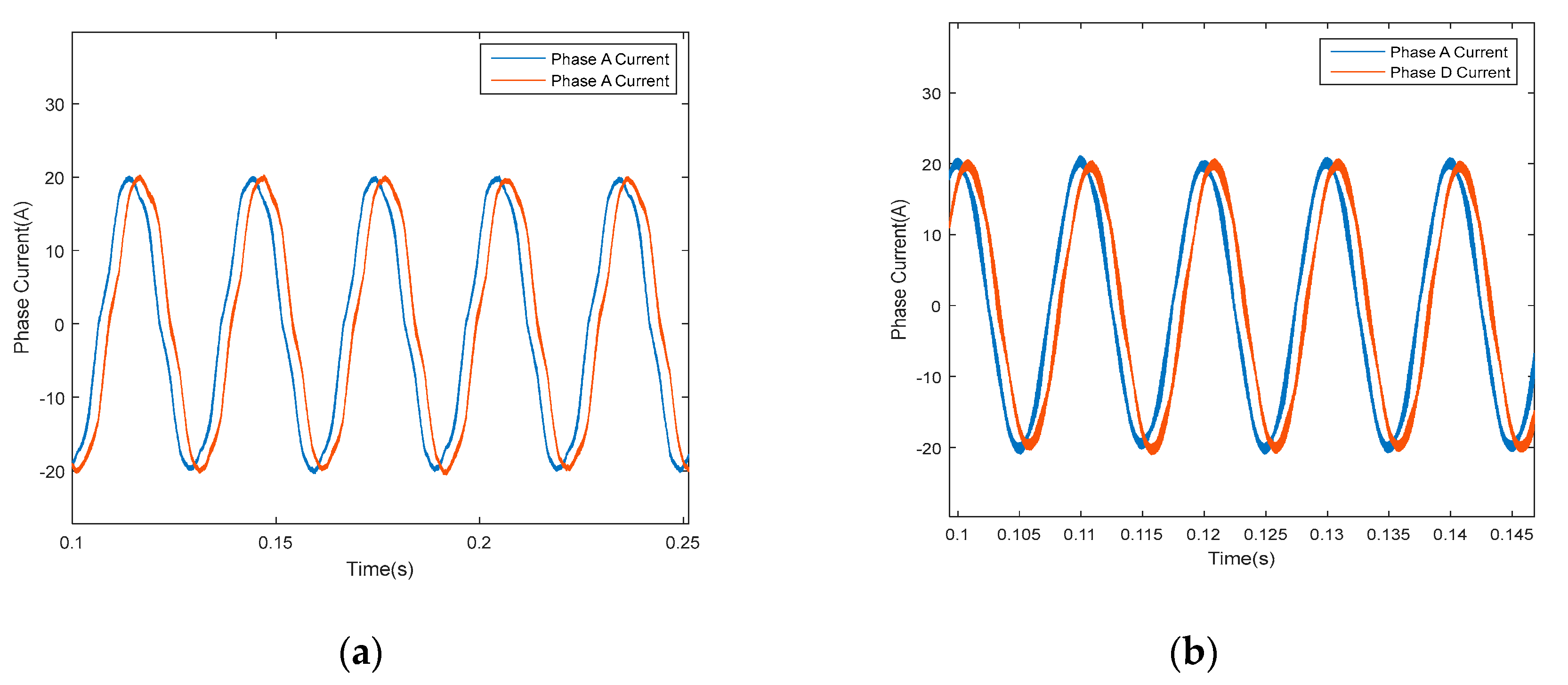
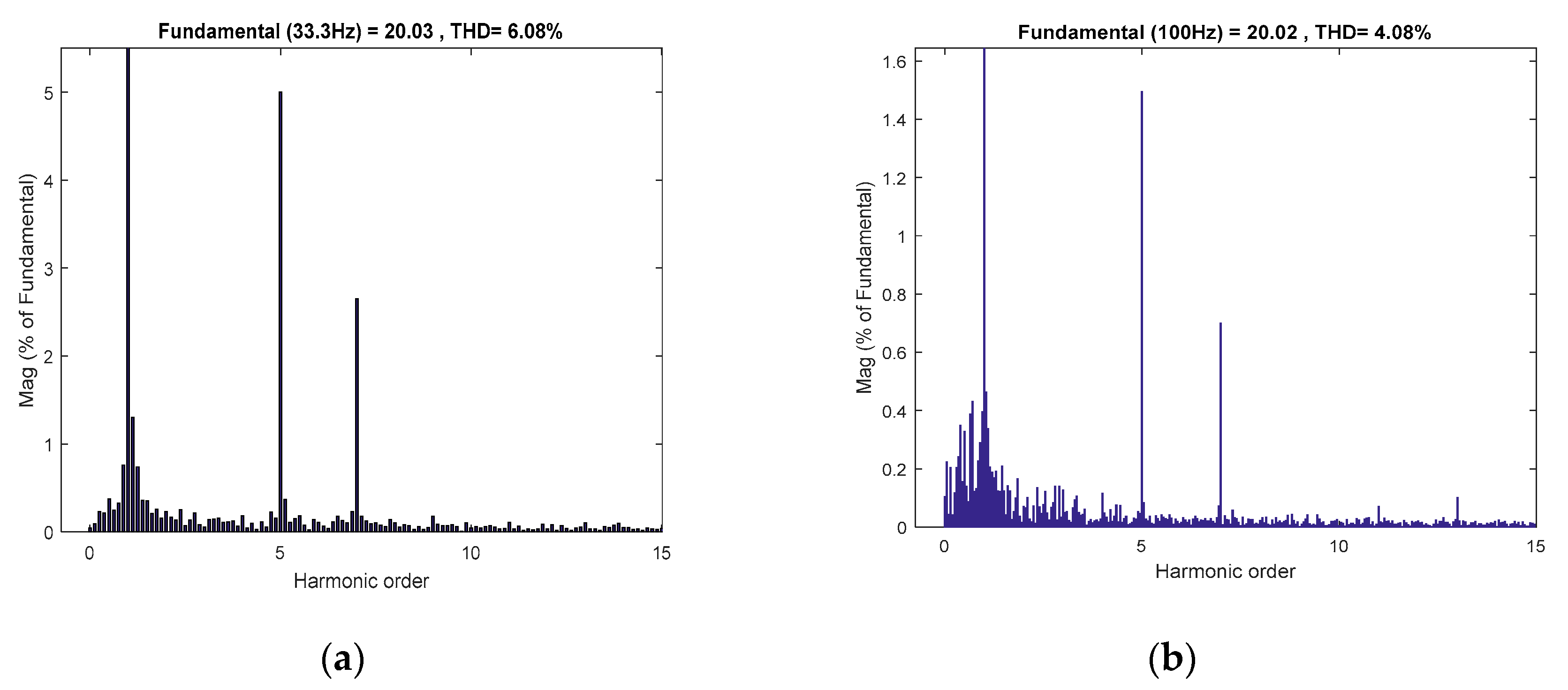
6.2. Validation of Current Regulator Design in Harmonic Subspace

Figure 13 shows the experimental results without employing the resonant controller when the command d- and q-axes currents are 0 A and 35 A, respectively. The speed of DT_PMSM is maintained at 500 r/min and 1500 r/min, respectively, and the values for u_x and u_y are zero. Figure 13 depicts that the phase currents are distorted severely because of the nonlinear characteristics of the inverter. As depicted in Figure 14, the fifth and seventh harmonics make up the majority of the harmonic currents and the total harmonic distortions (THDs) are 20.53% and 10.93%, respectively. In addition, the performances of the nonlinearities of the inverter are more evident at low speed than at high speed due to the fact that the voltage error caused by nonlinearities of the inverter constitutes a large portion at low speed.

Figure 15 illustrates the experimental performances after adopting the proposed resonant controller in x-y subspace. The compensating voltages are calculated based on the resonant controller and modulated by the suggested SVPWM scheme detailed in Section 5. The phase currents show better performances and the THDs of phase A current are decreased to 4.6% (500 r/min) and 3.34% (1500 r/min), respectively, as shown in Figure 16, after adopting the suggested scheme.

The speed of DT_PMSM is maintained at 500 r/min and 1500 r/min, respectively. The experimental performances are illustrated in Figure 17 without employing the resonant controller when the command currents of d- and q-axes are 0 A and 20 A, respectively. The values of u_x and u_y are 0. The THDs of phase A current are 23.27% and 16.10%, respectively, as illustrated in Figure 18. Moreover, at the same speed, the THD in this case is larger than the THD when the command currents of d- and q-axes are 0 A and 35 A because the fundamental component of phase current is smaller in this case.

On the contrary, after adopting the proposed resonant controller in harmonic subspace, the waveforms of phase currents have been improved a lot, as shown in Figure 19. The THDs are reduced to 6.08% and 4.08% when the speed is 500 r/min and 1500 r/min, respectively, as depicted in Figure 20.

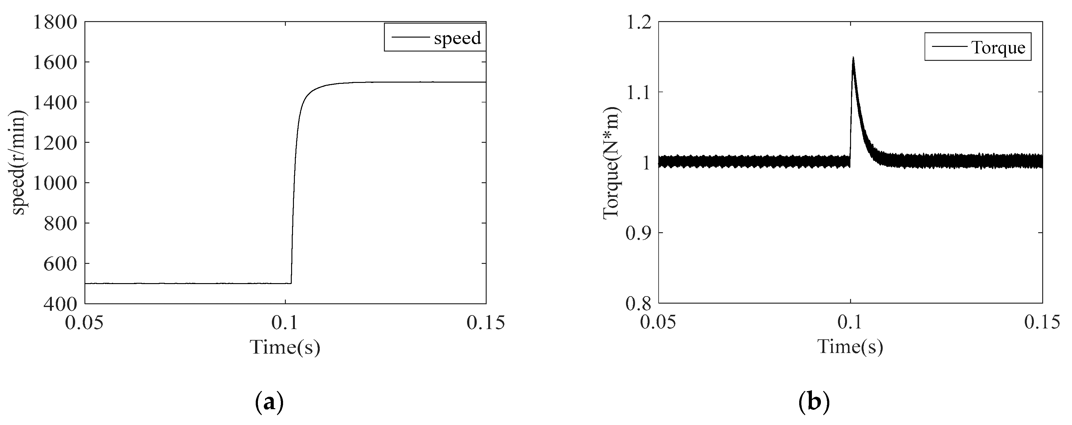
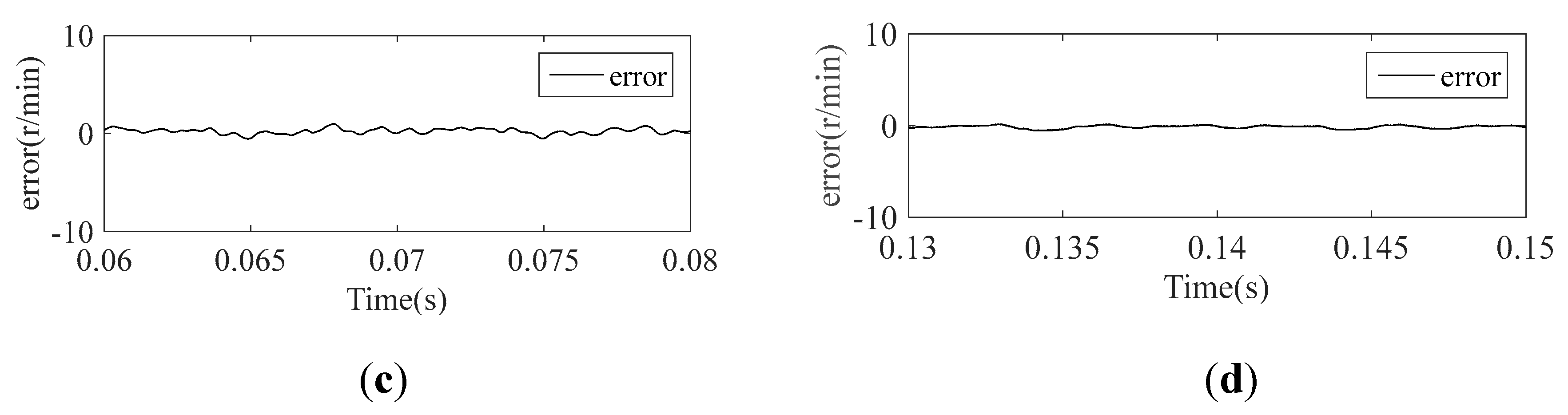
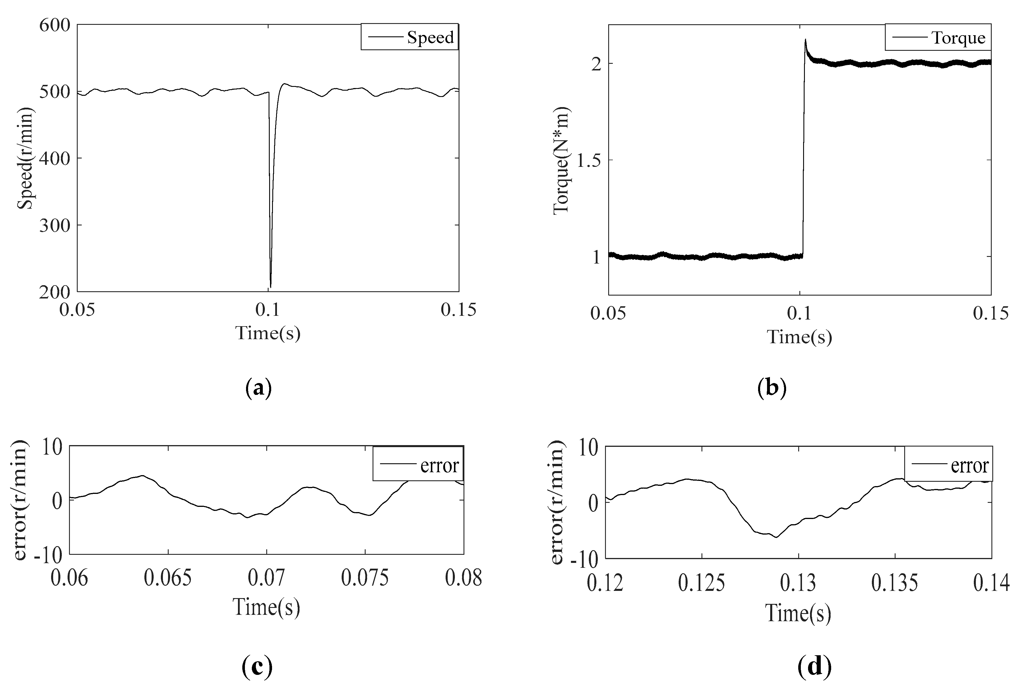
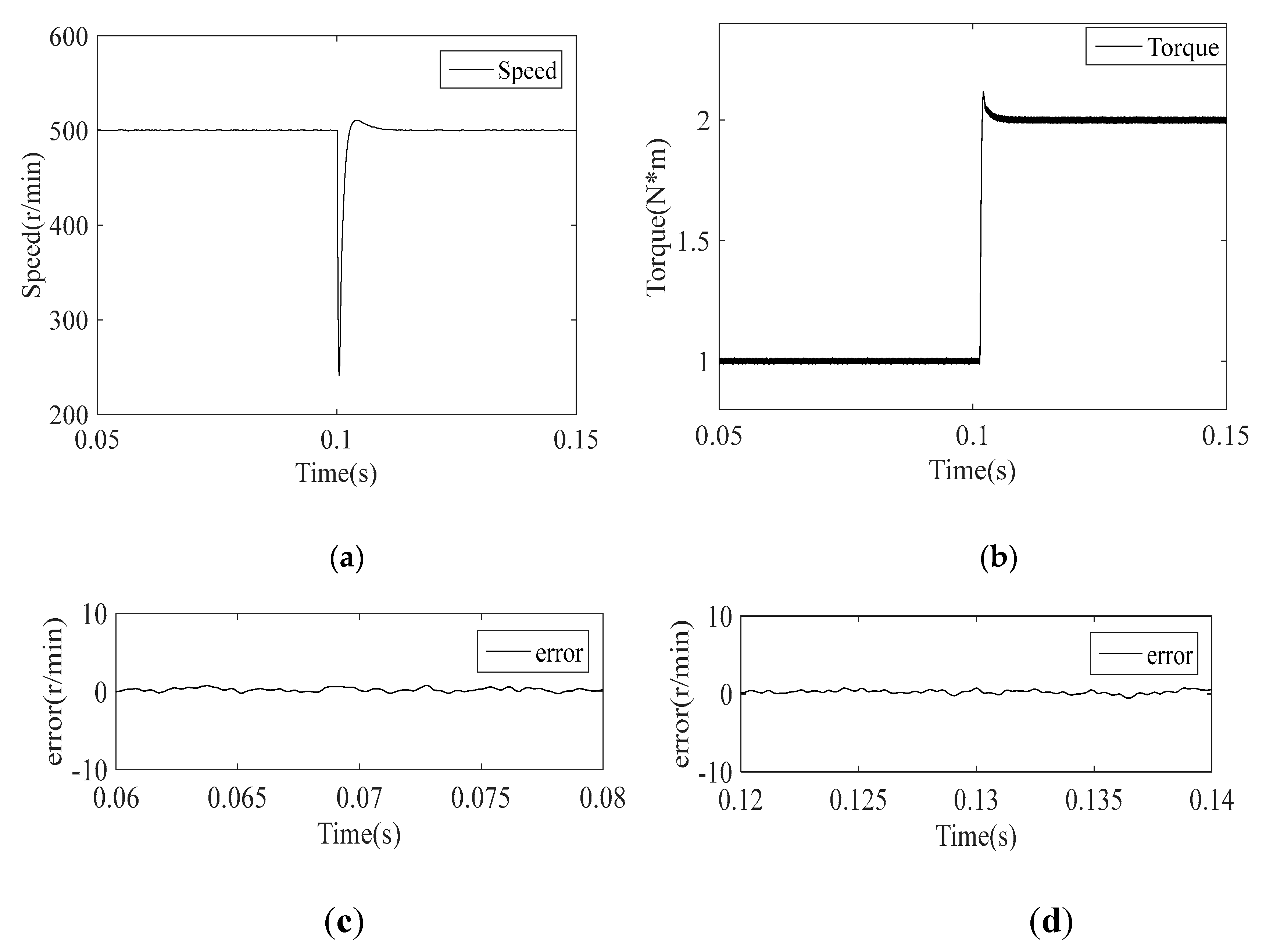
6.3. Performances under Speed Control Loop

Experiments are conducted under speed control loop to test the performances. The DT_PMSM is operating in the speed control loop and accelerates from 500 r/min to 1500 r/min under 1 N*m load conditions. The speed waveform, electromagnetic torque waveform and the speed fluctuation waveform, without and with the proposed current regulator design, are shown in Figure 21 and Figure 22, respectively.

From Figure 21 and Figure 22, it is clear that both strategies can follow the reference speed quickly and the settling time is nearly equal. The electromagnetic torque can also track the load torque quickly. However, small fluctuations can be found in the speed waveform and torque ripple is small based on the suggested current regulator, which means that the suggested current regulator shows better performances and can retain the advantages of rapid dynamic response.

The experiments are conducted when DT_PMSM is operating under a speed control loop and the load torque is a step change from 1 N*m to 2 N*m at 0.1 s. The reference speed is maintained at 500 r/min. The speed waveform, electromagnetic torque waveform and the speed fluctuation waveform, without and with the proposed current regulator design, are given in Figure 23 and Figure 24, respectively.

It can be seen from Figure 23 and Figure 24 that they can track the load torque quickly and the settling time is almost the same in both cases. Besides, the actual speed can follow the reference speed in both scenarios although the load torque changes. However, the speed waveform shows small fluctuations and the electromagnetic torque is smoother based on the suggested current regulator, which can also prove that the proposed current regulator can exhibit better performances and can have the merits of rapid dynamic response.

7. Conclusions

This paper gives the current regulator design for DT_PMSM on the basis of VSD theory. In α-β subspace, sliding mode control based on an internal model is proposed and in x-y subspace, a resonant controller based on a new synchronous rotating coordinate matrix is adopted to generate the compensation voltage without requiring additional hardware or a complicated signal processing algorithm. The three-phase decomposition SVPWM technique is adopted to modulate the voltage vectors in both subspaces simultaneously. The experimental results show that the current fluctuations of d- and q- axes are reduced. Furthermore, the harmonic currents are reduced. It can prove that the current regulator designed in α-β subspace is robust against variations of motor parameters and unknown disturbances and the current regulator designed in x-y subspace can suppress the harmonic currents effectively. In addition, the performances of speed and torque are compared with and without the suggested current regulator. It can be seen that smaller fluctuations can be found in the speed waveforms and smaller ripples can be found in the torque waveforms after adopting the proposed current regulator design, which also indicates that the suggested current regulator design can achieve better performances.

Future work will focus on discussing whether the suggested current regulator can be applied to a higher speed machine especially operating at the low frequency ratio.

References

1. Zheng, J.; Huang, S.; Rong, F.; Lye, M. Six-Phase Space Vector PWM under Stator One-Phase Open-Circuit Fault Condition. Energies 2018, 11, 1796. [Google Scholar] [CrossRef] [Green Version]
2. Levi, E. Multiphase Electric Machines for Variable-Speed Applications. IEEE Trans. Ind. Electron. 2008, 55, 1893–1909. [Google Scholar] [CrossRef]
3. Tounsi, K.; Djahbar, A.; Barkat, S. Extended Kalman Filter Based Sliding Mode Control of Parallel-Connected Two Five-Phase PMSM Drive System. Electronics 2018, 7, 14. [Google Scholar] [CrossRef] [Green Version]
4. Levi, E.; Bojoi, R.; Profumo, F.; Toliyat, H.A.; Williamson, S. Multiphase induction motor drives - a technology status review. IET Electr. Power Appl. 2007, 1, 489–516. [Google Scholar] [CrossRef] [Green Version]
5. Lipo, T.A. A d-q Model for Six Phase Induction Machines. In Proceedings of the International Conference Electrical Machine, Athens, Greece, 15–17 September 1980; pp. 860–867. [Google Scholar]
6. Wu, Z.; Gu, W.; Zhu, Y.; Lu, K. Current Control Methods for an Asymmetric Six-Phase Permanent Magnet Synchronous Motor. Electronics 2020, 9, 172. [Google Scholar] [CrossRef] [Green Version]
7. Zhao, Y.; Lipo, T.A. Space vector PWM control of dual three-phase induction machine using vector space decomposition. IEEE Trans. Ind. Appl. 1995, 31, 1100–1109. [Google Scholar] [CrossRef]
8. Rowan, T.M.; Kerkman, R.J. A New Synchronous Current Regulator and an Analysis of Current-Regulated PWM Inverters. IEEE Trans. Ind. Appl 1986, IA-22, 678–690. [Google Scholar] [CrossRef]
9. Harnefors, L.; Nee, H. Model-based current control of AC machines using the internal model control method. IEEE Trans. Ind. Appl. 1998, 34, 133–141. [Google Scholar] [CrossRef]
10. Briz, F.; Degner, M.W.; Lorenz, R.D. Analysis and design of current regulators using complex vectors. IEEE Trans. Ind. Appl. 2000, 36, 817–825. [Google Scholar] [CrossRef] [Green Version]
11. Holtz, J. Design of fast and robust current regulators for high-power drives based on complex state variables. IEEE Trans. Ind. Appl. 2004, 40, 1388–1397. [Google Scholar] [CrossRef]
12. Peters, W.; Böcker, J. Discrete-Time Design of Adaptive Current Controller for Interior Permanent Magnet Synchronous Motors (IPMSM) with High Magnetic Saturation. In Proceedings of the IECON 2013—39th Annual Conference of the IEEE Industrial Electronics Society, Vienna, Austria, 10–13 November 2013; pp. 6608–6613. [Google Scholar]
13. Altomare, A.; Guagnano, A.; Cupertino, F.; Naso, D. Discrete-Time Control of High-Speed Salient Machines. IEEE Trans. Ind. Appl. 2016, 52, 293–301. [Google Scholar] [CrossRef]
14. Lin, J.K. A new Approach of Dead-Time Compensation for PWM voltage inverters. IEEE Trans. Circuits Syst. I Fundam. Theory Appl. 2002, 49, 476–483. [Google Scholar]
15. Li, C. Analysis and Compensation of Dead-Time Effect Considering Parasitic Capacitance and Ripple Current. In Proceedings of the 2015 IEEE Applied Power Electronics Conference and Exposition (APEC), Charlotte, NC, USA, 15–19 March 2015; pp. 1501–1506. [Google Scholar]
16. Ryu, H.-M.; Kim, J.-W.; Sul, S.-K. Synchronous Frame Current Control of Multi-Phase Synchronous Motor —Part II Asymmetric Fault Condition due to Open Phases. In Proceedings of the Conference Record of the 2004 IEEE Industry Applications Conference, 2004. 39th IAS Annual Meeting, Seattle, WA, USA, 3–7 October 2004; p. 275. [Google Scholar]
17. Ryu, H.-M.; Kim, J.-W.; Sul, S.-K. Synchronous Frame Current Control of Multi-Phase Synchronous Motor. Part I. Modeling and Current Control Based on Multiple d-q Spaces Concept under Balanced Condition. In Proceedings of the Conference Record of the 2004 IEEE Industry Applications Conference, 2004. 39th IAS Annual Meeting, Seattle, WA, USA, 3–7 October 2004; p. 63. [Google Scholar]
18. Lascu, C.; Asiminoaei, L.; Boldea, I.; Blaabjerg, F. High Performance Current Controller for Selective Harmonic Compensation in Active Power Filters. IEEE Trans. Power Electron. 2007, 22, 1826–1835. [Google Scholar] [CrossRef]
19. Yepes, A.G.; Freijedo, F.D.; Lopez, Ó.; Doval-Gandoy, J. Analysis and Design of Resonant Current Controllers for Voltage-Source Converters by Means of Nyquist Diagrams and Sensitivity Function. IEEE Trans. Ind. Electron. 2011, 58, 5231–5250. [Google Scholar] [CrossRef]
20. Wu, Z.; Gu, W.; Lu, K.; Zhu, Y.; Guan, J. Current Harmonic Suppression Algorithm for Asymmetric Dual Three-Phase PMSM. Appl. Sci. 2020, 10, 954. [Google Scholar] [CrossRef] [Green Version]
21. Hadiouche, D.; Baghli, L.; Rezzoug, A. Space vector PWM Techniques for Dual Three-Phase AC Machine: Analysis, Performance Evaluation and DSP Implementation. In Proceedings of the 38th IAS Annual Meeting on Conference Record of the Industry Applications Conference, Salt Lake City, UT, USA, 12–16 October 2003; Volume 1, pp. 648–655. [Google Scholar]
22. Marouani, K.; Baghli, L.; Hadiouche, D.; Kheloui, A.; Rezzoug, A. A New PWM Strategy Based on a 24-Sector Vector Space Decomposition for a Six-Phase VSI-Fed Dual Stator Induction Motor. IEEE Trans. Ind. Electron. 2008, 55, 1910–1920. [Google Scholar] [CrossRef]
23. Bojoi, R.; Tenconi, A.; Profumo, F.; Griva, G.; Martinello, D. Complete Analysis and Comparative Study of Digital Modulation Techniques for Dual Three-Phase AC Motor Drives. In Proceedings of the 2002 IEEE 33rd Annual IEEE Power Electronics Specialists Conference, Proceedings (Cat. No.02CH37289), Cairns, QLD, Australia, 23–27 June 2002; Volume 2, pp. 851–857. [Google Scholar]
24. Zhou, C.; Yang, G.; Su, J. PWM Strategy With Minimum Harmonic Distortion for Dual Three-Phase Permanent-Magnet Synchronous Motor Drives Operating in the Overmodulation Region. IEEE Trans. Power Electron. 2016, 31, 1367–1380. [Google Scholar] [CrossRef]
Figure 1. Phase winding diagram for a dual Y shift 30 degrees permanent magnet synchronous motor (DT_PMSM).
Electronics 09 00777 g001
Figure 2. Driving system of DT_PMSM.
Electronics 09 00777 g002
Figure 3. Block diagram of internal model control.
Electronics 09 00777 g003
Figure 4. Block diagram of current regulator based on internal model.
Electronics 09 00777 g004
Figure 5. Block diagram of current regulator based on internal model.
Electronics 09 00777 g005
Figure 6. Block diagram of resonant controller.
Electronics 09 00777 g006
Figure 7. Block diagram of resonant controller with compensation angle.
Electronics 09 00777 g007
Figure 8. Pulse Width Modulation (PWM) Strategy for DT_PMSM.
Electronics 09 00777 g008
Figure 9. Control diagram of control scheme for DT_PMSM.
Electronics 09 00777 g009
Figure 10. Experimental set-up for DT-PMSM.
Electronics 09 00777 g010
Figure 11. Experimental results based on the traditional internal model control method in α-β subspace, (a) d-axis current and (b) q-axis current.
Electronics 09 00777 g011
Figure 12. Experimental results after adopting the proposed control method in α-β subspace, (a) d-axis current and (b) q-axis current.
Electronics 09 00777 g012
Figure 13. Phase currents without adopting the resonant controller in x-y subspace, (a) running at 500 r/min and (b) running at 1500 r/min.
Electronics 09 00777 g013
Figure 14. Total harmonic distortion (THD) of phase A Current, (a) running at 500 r/min and (b) running at 1500 r/min.
Electronics 09 00777 g014
Figure 15. Phase currents after adopting the suggested control algorithm in x-y subspace, (a) running at 500 r/min and (b) running at 1500 r/min.
Electronics 09 00777 g015
Figure 16. THD of phase A Current, (a) running at 500 r/min and (b) running at 1500 r/min.
Electronics 09 00777 g016
Figure 17. Phase currents without adopting the proposed algorithm in x-y subspace, (a) running at 500 r/min and (b) running at 1500 r/min.
Electronics 09 00777 g017
Figure 18. THD of phase A Current, (a) running at 500 r/min and (b) running at 1500 r/min.
Electronics 09 00777 g018
Figure 19. Phase currents after adopting the proposed algorithm in x-y subspace, (a) running at 500 r/min and (b) running at 1500 r/min.
Electronics 09 00777 g019
Figure 20. THD of phase A Current, (a) running at 500 r/min and (b) running at 1500 r/min.
Electronics 09 00777 g020
Figure 21. Waveforms after a speed step change from 500 r/min to 1500 r/min under 1 N*m load conditions without the proposed current regulator. (a) Speed response. (b) Electromagnetic torque response. (c) Error between the actual speed and reference speed (the reference speed is 500 r/min). (d) Error between the actual speed and reference speed (the reference speed is 1500 r/min).
Electronics 09 00777 g021
Figure 22. Waveforms after a speed step change from 500 r/min to 1500 r/min under 1 N*m load condition with the proposed current regulator. (a) Speed response. (b) Electromagnetic torque response. (c) Error between the actual speed and reference speed (the reference speed is 500 r/min). (d) Error between the actual speed and reference speed (the reference speed is 1500 r/min).
Electronics 09 00777 g022aElectronics 09 00777 g022b
Figure 23. Waveforms after a load torque change from 1 N*m to 2 N*m without the proposed current regulator. The reference speed is 500 r/min. (a) Speed response. (b) Electromagnetic torque response. (c) Error between the actual speed and reference speed (load torque is 1 N*m). (d) Error between the actual speed and reference speed (load torque is 2 N*m).
Electronics 09 00777 g023
Figure 24. Waveforms after a load torque change from 1 N*m to 2 N*m with the proposed current regulator. The reference speed is 500 r/min. (a) Speed response. (b) Electromagnetic torque response. (c) Error between the actual speed and reference speed (load torque is 1 N*m). (d) Error between the actual speed and reference speed (load torque is 2 N*m).
Electronics 09 00777 g024