Abstract
Driving fatigue accounts for a large number of traffic accidents in modern life nowadays. It is therefore of great importance to reduce this risky factor by detecting the driver’s drowsiness condition. This study aimed to detect drivers’ drowsiness using an advanced electroencephalography (EEG)-based classification technique. We first collected EEG data from six healthy adults under two different awareness conditions (wakefulness and drowsiness) in a virtual driving experiment. Five different machine learning techniques, including the K-nearest neighbor (KNN), support vector machine (SVM), extreme learning machine (ELM), hierarchical extreme learning machine (H-ELM), and the proposed modified hierarchical extreme learning machine algorithm with particle swarm optimization (PSO-H-ELM), were applied to classify the subject’s drowsiness based on the power spectral density (PSD) feature extracted from the EEG data. The mean accuracies of the five classifiers were 79.31%, 79.31%, 74.08%, 81.67%, and 83.12%, respectively, demonstrating the superior performance of our new PSO-H-ELM algorithm in detecting drivers’ drowsiness, compared to the other techniques.
1. Introduction
The rapid development of industrial technology has turned cars into a popular means of transportation. Simultaneously, the fierce competition in modern society pushes people to work hard, leading to excessive fatigue in daily life. Working under fatigue not only decreases overall efficiency, but also damages bodily health and can even cause accidents [1]. In recent years, fatigue driving has emerged as a major cause of traffic accidents. Drivers attempting to travel long distances often operate their vehicle in a fatigued or drowsy condition. In addition, driving time is not the only cause of fatigue; other factors, for instance, monotonous environments, sleep deprivation, chronic sleepiness, and drug and alcohol use are also related to fatigue [2,3]. Driving fatigue can lead to devastating accidents, especially in cases where drivers fall asleep while the car is still moving. Drowsiness detection is therefore an important topic in the field of driving safety, with the aim of decreasing the frequency and severity of traffic accidents.
Over the last few decades, increasing efforts have been made to investigate the effective detection of driving fatigue, resulting in a number of methods being proposed for this particular application [4]. At present, the primary fatigue detection methods mainly comprise three categories. The first category generally focuses on behavioral features by detecting the variability of lateral lane position and vehicle heading difference to monitor the driver’s mental condition [5]. This approach is conceptually straightforward, but a standard for these features has not yet been well established, rendering it difficult to implement. Image-based facial expression recognition, such as the degree of resting eye closure or nodding frequency, represents the second type of approach for detecting driving fatigue [6,7]. Although these measures are easy to use, the detection of fatigue-linked features is subject to multiple factors, including image angle and image illumination, which lower their overall identification accuracy and limit their effectiveness in practical applications. The third type of approach mainly relies on physiological features, including electrocardiogram (ECG), heart rate [8], electromyogram (EMG), and electroencephalogram (EEG)-based features to detect driving fatigue [9]. Unlike the behavioral and facial features, physiological features serve as objective markers of inherent changes in the human body in response to surrounding conditions. Among these signals, EEG is considered to be the most straightforward, effective, and suitable one for detecting driving fatigue [10].
The most accessible equipment for collecting EEG signals is a wearable EEG acquisition device that allows a portable setup to be applied to measure EEG signals and determine whether the driver is in a fatigued condition or not. Classification algorithms, for instance, K-nearest neighbor (KNN) and support vector machine (SVM), are commonly used in this field. The classification efficiency of these classifiers, however, is not ideal due to the complexity of computation. As a result, in recent years some research groups have turned to algorithms that feature high computational efficiency, such as the extreme learning machine (ELM) [11]. However, the shallow architecture of the ELM may render it ineffective when attempting to learn features from natural signals, regardless of the quantity of hidden nodes. Considering this issue, an enhanced ELM-based hierarchical learning algorithm framework has been proposed by Huang et al. [12], known as a hierarchical extreme learning machine (H-ELM). When compared with other multilayer perceptron (MLP) training approaches, such as the traditional ELM, the H-ELM has a faster training speed as well as higher accuracy. The high-level representation achieved by the H-ELM primarily benefits from a layer-wise encoding architecture which extracts multilayer sparse features from the input data. A detailed description of this method will be provided in Section 2.6 Conversely, the L2 penalty and the scaling factor of the H-ELM classifiers are usually chosen according to empirical data, ignoring the importance of optimizing the parameters and performance of the classifier. Therefore, there is clearly a need to improve the performance of H-ELM by selecting optimal parameters.
Taking these together, in this study we proposed a new algorithm based on the H-ELM classifier and the particle swarm optimization (PSO) algorithm to improve classification accuracy. The PSO algorithm has been previously proven to be able to effectively select the best parameters for the classifiers [13]. By combining the PSO with the unique characteristics of EEG signals, the parameters of the H-ELM kernel function can be optimized, thereby improving the performance of driving fatigue detection.
2. Materials and Methods
2.1. Participants
Six male volunteers (right-handed, average age 24 years) with valid drivers’ licenses were recruited to participate in a simulated driving experiment. The research ethics board of Hangzhou Dianzi University approved the experiment and it was performed according to the Declaration of Helsinki. All subjects were physically and psychologically healthy, with regular sleep patterns.
2.2. Experiment
In this study, we used driving simulation equipment with related software to simulate the real driving scenario. The platform was an advanced simulation system (Shanghai Infrared Automobile Simulator Driving Equipment Co., Ltd, Shanghai, China), which can simulate surrounding scenes as well as the response of driving. The driving simulation platform consisted of a steering wheel, brake and accelerator pedals, a high-definition monitor, a high-performance computer with driving simulation software, and EEG signal recording equipment (Brain Products GmbH, Germany). The platform was established to dynamically record EEG signals during the experiment and monitor vehicle driving as well as operating status.
In order to obtain EEG data for fatigue and awake states, each subject was required to sleep for four hours (sleep deprivation) or eight hours (adequate sleep), respectively, on the day immediately before the collection of EEG data. As such, EEG data were collected twice from each participant separately. The experiments were designed to start at 9:00 a.m. uniformly on each experimental day as scheduled, and the EEG data were recorded continuously for 20 min during the driving in the driving simulation environment. Specifically, in order to induce drowsiness in the subjects in the fatigue group, we chose a long highway that was straight with smooth curves. Conversely, the road for the awake group was relatively complex to keep the subjects awake. During the experiment, we evaluated the subject’s drowsiness using a micro-camera based on the driving fatigue criteria (more than two seconds’ eye closure, head nodding, and large deviation off the road) described in the literature [14,15].
2.3. EEG Data Acquisition
In our experiment, subjects were required to sit on a chair and drive on the simulation platform while EEG signals were recorded from 32 EEG electrodes positioned on each subject’s head surface with a sampling rate of 1000 Hz. EEG data for the fatigue group were recorded for 20 min after the subjects had fatigue symptoms. For the subjects who did not show fatigue symptoms after 60 min driving, the experiments were resumed a few days later. The temperature of the laboratory was maintained at 22 °C, which was suitable for the subjects. Figure 1 shows the driving simulation platform of our experiment.
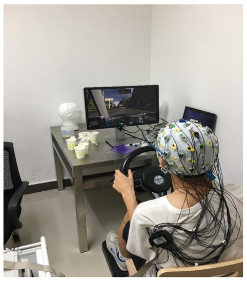
Figure 1.
The experimental setup with the driving platform and electroencephalogram (EEG) recording system.
2.4. Data Preprocessing
Raw EEG data were first down-sampled to 200 Hz. A 4th-order band-pass filter (0.1 to 45 Hz) was applied to reduce noise during the EEG recording, including electrode resistance, drift, sweating, powerline interference, white noise, and EMG (the frequency of unrelated EMG signals produced by a muscle contraction is usually greater than 100 Hz [16]). Finally we filtered the EEG signals to obtain five traditional EEG frequency bands, including Delta (0.1–4 Hz), Theta (4–8 Hz), Alpha (8–13 Hz), Beta (13–20 Hz), and Gamma (20–45 Hz) [17]. The distribution of frequency bands changed over time, and the appearance of frequency bands can be used as a feature associated with fatigue [18,19].
In this study we defined a 10-s segment of EEG data as a sample, creating 240 samples for each subject and 1440 samples in each group. Among these, 240 samples from one subject were set aside as a testing set, while the remaining 1200 samples from the other five subjects were used as a training set.
2.5. Feature Extraction
Features were then extracted from the preprocessed and segmented EEG samples. In this study we adopted the power spectral density (PSD) of the EEG samples as features since they represent the distribution of the EEG frequencies. The PSD values were computed by short-time Fourier transforms (STFT) for each EEG channel and each frequency band. A total of 160 PSD datapoints (32 electrodes × 5 frequency bands) were thereby extracted for each EEG sample. Specifically, we adopted a Hanning window-based discrete STFT algorithm to extract the PSD features.
Briefly, for the EEG signal recorded by an electrode, denoted as , the STFT of the EEG signal is given as:
where is the angular frequency and . In this case, m represents the width of windows function in time domain, m is discrete and ω is continuous, is a window function, N represents the number of sampling point. The definition equation of a Hanning window is as follows:
The Fourier transform equation is given as:
where is a conjugate function of , is essentially the discrete STFT as shown in Equation (1), and PSD is defined as:
The energy spectrum of each EEG frequency band could then be defined as:
where represent all the frequencies in one frequency band.
Figure 2 shows an example of the comparison of raw EEG signals and the PSD between the awake and fatigue stages. Ten-second recorded EEG signals recorded from a participant from the awake group and fatigue group, respectively, and their PSD were compared. For the original signal, the x-axis represents the datapoint, and the y-axis represents the amplitude. For the PSD signal, the x-axis represents the frequency, and the y-axis represents the signal’s power content versus frequency. It can be seen that it is easier to distinguish the fatigue state from the awake state in the frequency domain, and the main distinction is concentrated between 0 and 40 Hz.
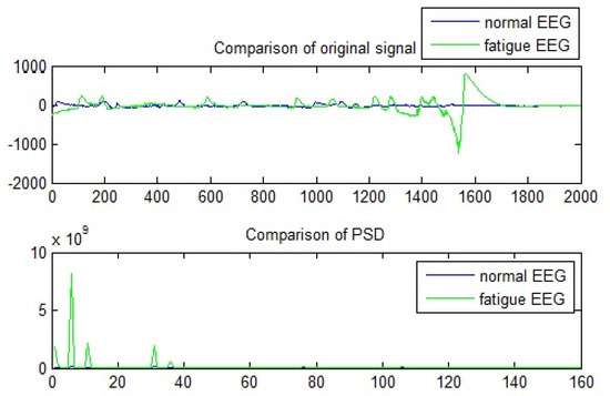
Figure 2.
The comparison of raw EEG signals and their power spectral density (PSD) between the awake and fatigue stages.
2.6. Classical ELM and PSO-H-ELM
The classical extreme learning machine (ELM) was proposed for classification or regression tasks. It is a feedforward neural network with a single layer of hidden nodes. The weights connecting each node were assigned randomly initially. Specifically, the weights between input neurons and hidden nodes were instant, while the weights between hidden nodes and output neurons upgraded gradually by the linear model. This design accelerates the learning speed greatly with favorable generalization performance.
Assume there are samples in a training set , where represents each sample and its corresponding network target vector is . The classical single hidden layer feedforward neural network (SLFN) is mathematically defined as:
where represents hidden nodes, is activation function, represents the weight vector connecting the th hidden node with input neurons, the weight vector between the th hidden node and the output nodes is defined by , and is the bias of the th hidden node. is the nonlinear activation function, for instance, a sigmoid or Gaussian function. The standard SLFNs can approximate the target output with zero error means.
For convenience, this equation could be written compactly as:
where and .
In this definition, is a feature mapping function which turns the -dimensional data into the -dimensional feature, and represent the factors of the mapping function.
The original ELM algorithm approximates target output by adjusting weights connecting input and hidden layer as well as biases of hidden nodes. Specifically, the weights are filled with random values when the activation function is infinitely differentiable.
According to the above introduction, the initial hidden nodes of the original ELM algorithm are assigned randomly. When it comes to a multilayer perceptron (MLP), the ELM algorithm needs to combine the auto encoder function. The auto encoder function extracts hidden features through the feature map, with which ELM could approximate the output by minimizing error. The framework of H-ELM is multilayer, as presented in Figure 3. Every circle illustrated in Figure 3 represents a neuron of a neural network, and every matrix of those circles represents a hidden layer. The last column in Figure 3 is the prediction of H-ELM framework.
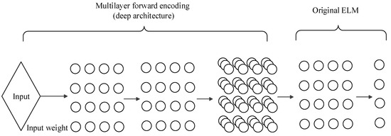
Figure 3.
The overall framework of the hierarchical extreme learning machine (H-ELM) learning algorithm.
Normally, deep learning algorithms apply greedy layer-wise architecture to train the data, while the H-ELM algorithm divides it into two separate phases. The first phase refers to the processing of unsupervised hierarchical feature representation. Through the process of unsupervised learning within the new ELM-based auto encoder, we could transform the input into a random feature space. This could be aided by taking advantage of the hidden feature of training data. The auto encoder is designed through using a sparse constraint with an added approximation capability, and is therefore known as the ELM sparse auto encoder. Each hidden layer of the H-ELM works like an individual unit which extracts features; increasing the number of layers in this method will consequently increase the number of extracted features. By adopting an -layer unsupervised learning method, the H-ELM algorithm obtains higher sparse features. The output of each hidden layer is shown as:
where represents the output of the th layer, represents the output of the th layer, represents the activation function, and is the output weights.
The output weights are calculated as:
where is the hidden layer outputs matrix and are output data. The L2 penalty C is preset to balance the distance of separating margin and the training error [20].
Specifically, the value of L1 is optimized in order to extract more sparse hidden features, which is different from reference [21] where L2-norm singular values are optimized.
The next phase of H-ELM is supervised feature classification. Specifically, we applied the traditional ELM regression for the classification. The auto encoder approximates the inputs to outputs through the least mean square method, while the H-ELM algorithm offers a better solution with improved accuracy and speed. In this phase, the scaling factor S is used to adjust the max value of training output, and the value of s is specified by the user.
Figure 4 depicts the testing accuracies of H-ELM in the C and S subspaces, and it can be seen that the performance of H-ELM is obviously related to parameters C and S. It is therefore of great value to select the most appropriate values for these two parameters by using optimization algorithms to achieve the best performance of H-ELM. In this study we adopted particle swarm optimization (PSO) to optimize the H-ELM algorithm.
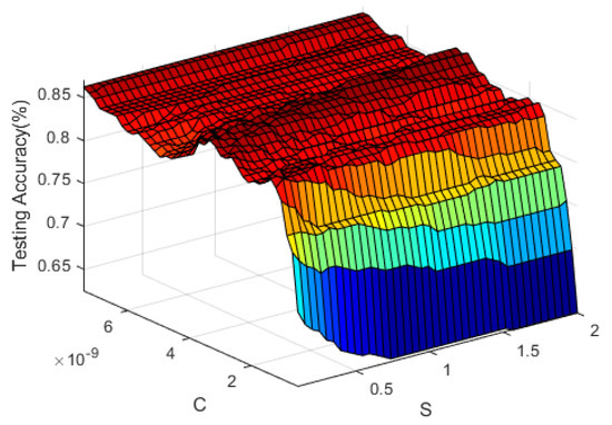
Figure 4.
Testing accuracy in (C, S) subspace for the H-ELM.
The PSO is one of the ‘swarm intelligence techniques’, which are proposed by the observation of biotic communities in nature. The PSO algorithm itself was based on the Boid model, which imitates the flying behavior of bird flocks [22,23]. With the PSO model, each particle’s position is described by a position vector and speed vector, which respectively represent the solutions of problem and movement within the search space. The particles remember the best position where they reached the highest accuracy during their past states and use this information to guide their search of the solution space.
The kernel of the PSO algorithm contains constantly updated values for the speed and position of each particle. These equations are defined as:
where is the inertia weight, and are the acceleration constants, and are uniformly distributed random numbers between , represents the speed of the th dimension of th particle of the th generation. describes the best position of the th dimension of th particle of the th generation, while represents the best position of the whole swarm.
In this part, we adopted the classic PSO algorithm to find the best L2 penalty for the last layer of the ELM as well as the best scaling factor for the original ELM. Root mean squared error (RMSE) is a common criterion to measure the performance of classification or regression. Mathematically, the RMSE is defined as:
where is the target of training data, represents the output, and represents the number of subjects.
2.7. Classification
In order to evaluate the performance of the proposed PSO-H-ELM, in this study we tested the classification performance in the driving fatigue detection using five different classifiers, including the K-nearest neighbor (KNN), support vector machine (SVM), extreme learning machine (ELM), hierarchical extreme learning machine (H-ELM), and the proposed PSO-H-ELM. The KNN, ELM, and, especially, SVM, are all widely used in the field. As mentioned above, 240 samples from one subject were defined as the testing data, whereas the remaining 1200 samples of the five other subjects were training data. This arrangement was adopted to avoid any possible confounds from the random selection of training and test data. All processing was implemented in the MATLAB 2017a environment on a PC with a 3.4 GHz processor and 8.0 GB RAM.
3. Results
In this study, the initial values of C and S were set to 2 × 10⁻³⁰ and 0.8, respectively. The inertia weight was 0.6 and the acceleration constants and were set to 1.6 and 1.5, respectively. The number of particles was set to 1000, and the maximum number of population iterations was set to 20.
Figure 4 summarizes the performance of five classifiers in the classification of driving fatigue across all subjects. Briefly, the KNN model achieved accuracies of 72.08%, 74.17%, 90.00%, 93.33%, 74.58%, and 71.67%, respectively. Use of the SVM resulted in accuracies of 77.50%, 76.67%, 89.58%, 95.83%, 62.92%, and 73.33%, respectively. The ELM demonstrated accuracies of 70.58%, 69.58%, 86.25%, 88.75%, 58.75%, and 67.25%, respectively. Use of the H-ELM resulted in accuracies of 79.17%, 82.08%, 90.42%, 90.83%, 72.08%, and 75.42%, respectively. Finally, the PSO-H-ELM achieved accuracies of 80.01%, 84.58%, 92.50%, 92.08%, 73.33%, and 76.25%, respectively. Together, the performances achieved by different algorithms changed drastically across subjects, making it difficult to determine the optimal approach for driving fatigue detection.
Average accuracies for the five classifiers were calculated and presented in Figure 5. We further performed paired t-tests to determine if the performance of the PSO-H-ELM significantly outperforms other classifiers.
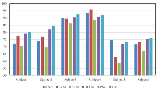
Figure 5.
The classification accuracies achieved by K-nearest neighbor (KNN), support vector machine (SVM), extreme learning machine (ELM), H-ELM, and proposed modified hierarchical extreme learning machine algorithm with particle swarm optimization (PSO-H-ELM) with respect to different training subjects.
4. Discussion
As shown in Figure 6, the PSO-H-ELM algorithm achieved the highest average accuracy, indicating that the proposed PSO-H-ELM is superior to others in the detection of driving fatigue. By comparing the performance of H-ELM with the proposed PSO-H-ELM in different cases, we found that the selection of training data has no appreciable influence on the performance of the proposed algorithm. Despite exhibiting a higher mean accuracy in the proposed PSO-H-ELM, no significant differences were found between the proposed PSO-H-ELM and the KNN and SVM. Significant differences were found, however, when the PSO-H-ELM was compared to the ELM and H-ELM algorithms, indicating that the optimization of the L2 penalty and scaling factor does improve the performance of the H-ELM algorithm. The results of the statistical analysis are shown in Table 1.
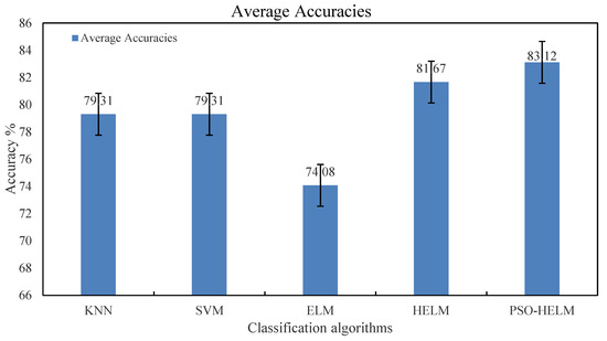
Figure 6.
The average classification accuracies achieved by KNN, SVM, ELM, H-ELM, and PSO-H-ELM.

Table 1.
Comparison of accuracies of classifiers.
Across traditional classification methods tested in this study, the H-ELM outperforms the SVM. With the addition of the PSO algorithm, the PSO-H-ELM further optimizes the performance of the classifier in fatigue detection, which provides inspiration for other studies.
5. Limitations
One of the limitations of this pilot study was the small sample size (n = 6). Our human experiment has been suspended due to the COVID-19 outbreak. The promising results achieved based on such a small sample size, however, enable important adjustments for a large-scale future study when the situation allows.
6. Conclusions
In this pilot study, we have presented an algorithm for driving fatigue detection based on the H-ELM and PSO algorithms, and provided evidence that the proposed PSO-H-ELM outperformed the existing classification algorithms. It is noteworthy that the proposed method differed from the H-ELM by adopting the PSO approach to optimize the key parameters when using H-ELM and thereby achieved better classification accuracy. In particular, as a classifier, PSO-H-ELM achieved more robust and accurate results compared to the other classifiers. The only known drawback is that the PSO-H-ELM requires a longer time for training, though this lack of training speed can be improved in future studies. A future study should be devoted to reducing the number of electrodes so that the acquisition of EEG signals is more convenient. In addition, other tools or features which could be used to better evaluate the cognitive state during driving could be explored to further improve the classification accuracy.
Author Contributions
For research articles with several authors, a short paragraph specifying their individual contributions must be provided. conceptualization, S.Z. and Y.M.; methodology, S.Z. and Y.Z.; software, S.Z. and D.Q.; validation, S.Z., R.L. and T.P.; formal analysis, D.Q. and R.L.; investigation, S.Z. and Z.L.; resources, Y.M. and Y.Z.; data curation, S.Z.; writing—Original draft preparation, S.Z. and Y.M.; writing—Review and editing, T.P. and R.L.; visualization, S.Z.; supervision, Y.M. and Y.Z.; project administration, Y.M.; funding acquisition, Y.M. and Z.L. All authors have read and agreed to the published version of the manuscript.
Funding
This research was funded by the National Natural Science Foundation of China grant number 61372023, 61671197 And the APC was funded by 61372023.
Conflicts of Interest
The authors declare no conflict of interest.
References
- Zhang, G.; Yau, K.K.; Zhang, X.; Li, Y. Traffic accidents involving fatigue driving and their extent of casualties. Accid. Anal. Prev. 2016, 87, 34–42. [Google Scholar] [CrossRef]
- Nilsson, T.; Nelson, T.M.; Carlson, D. Development of fatigue symptoms during simulated driving. Accid. Anal. Prev. 1997, 29, 479–488. [Google Scholar] [CrossRef]
- Ting, P.-H.; Hwang, J.-R.; Doong, J.-L.; Jeng, M.-C. Driver fatigue and highway driving: A simulator study. Physiol. Behav. 2008, 94, 448–453. [Google Scholar] [CrossRef] [PubMed]
- Milosevic, S. Drivers’ fatigue studies. Ergonomics 1997, 40, 381–389. [Google Scholar] [CrossRef]
- Morris, D.M.; Pilcher, J.J.; Switzer Iii, F.S. Lane heading difference: An innovative model for drowsy driving detection using retrospective analysis around curves. Accid. Anal. Prev. 2015, 80, 117–124. [Google Scholar] [CrossRef] [PubMed]
- D’Orazio, T.; Leo, M.; Guaragnella, C.; Distante, A. A visual approach for driver inattention detection. Pattern Recognit. 2007, 40, 2341–2355. [Google Scholar] [CrossRef]
- LBergasa, M.; Nuevo, J.; Sotelo, M.A.; Barea, R.; Lopez, M.E. Real-time system for monitoring driver vigilance. IEEE Trans. Intell. Transp. Syst. 2006, 7, 63–77. [Google Scholar] [CrossRef]
- Healey, J.A.; Picard, R.W. Detecting Stress during Real-World driving Tasks using Physiological Sensors. IEEE Trans. Intell. Transp. Syst. 2005, 6, 156–166. [Google Scholar] [CrossRef]
- Fu, R.; Wang, H. Detection of driving fatigue by using noncontact EMG and ECG signals measurement system. Int. J. Neural Syst. 2014, 24, 1450006. [Google Scholar] [CrossRef] [PubMed]
- Lin, C.T.; Ko, L.W.; Lin, K.L.; Liang, S.F.; Kuo, B.C.; Chung, I.F.; Van, L.D. Classification of Driver’s Cognitive Responses Using Nonparametric Single-trial EEG Analysis. In Proceedings of the 2007 IEEE International Symposium on Circuits and Systems, New Orleans, LA, USA, 27–30 May 2007; pp. 2019–2023. [Google Scholar]
- Huang, G.B.; Zhu, Q.Y.; Siew, C.K. Extreme learning machine: Theory and applications. Neurocomputing 2006, 70, 489–501. [Google Scholar] [CrossRef]
- Tang, J.; Deng, C.; Huang, G.B. Extreme Learning Machine for Multilayer Perceptron. IEEE Trans. Neural Netw. Learn. Syst. 2016, 27, 809. [Google Scholar] [CrossRef] [PubMed]
- Shi, Y.; Eberhart, R. Modified particle swarm optimizer. In Proceedings of the 1998 IEEE International Conference on Evolutionary Computation Proceedings. IEEE World Congress on Computational Intelligence (Cat. No.98TH8360), Anchorage, AK, USA, 4–9 May 1999; pp. 69–73. [Google Scholar]
- Chai, R.; Naik, G.R.; Nguyen, T.N.; Ling, S.H.; Tran, Y.; Craig, A.; Nguyen, H.T. Driver Fatigue Classification with Independent Component by Entropy Rate Bound Minimization Analysis in an EEG-Based System. IEEE J. Biomed. Health Inform. 2017, 21, 715–724. [Google Scholar] [CrossRef] [PubMed]
- Nguyen, T.; Ahn, S.; Jang, H.; Jun, S.C.; Kim, J.G. Utilization of a combined EEG/NIRS system to predict driver drowsiness. Sci. Rep. 2017, 7, 43933. [Google Scholar] [CrossRef] [PubMed]
- Komi, P.V.; Tesch, P. EMG frequency spectrum, muscle structure, and fatigue during dynamic contractions in man. Eur. J. Appl. Physiol. Occup. Physiol. 1970, 42, 41–50. [Google Scholar] [CrossRef] [PubMed]
- Deuschl, G.; Eisen, A. Recommendations for the Practice of Clinical Neurophysiology: Guidelines of the International Federation of Clinical Neurophysiology; Elsevier Health Sciences: Amsterdam, The Netherlands, 1999. [Google Scholar]
- Lin, C.T.; Wu, R.C.; Liang, S.F.; Chao, W.H.; Chen, Y.J.; Jung, T.P. EEG-based drowsiness estimation for safety driving using independent component analysis. IEEE Trans. Circuits Syst. I Regul. Pap. 2015, 52, 2726–2738. [Google Scholar]
- Jung, T.P.; Makeig, S.; Stensmo, M.; Sejnowski, T.J. Estimating alertness from the EEG power spectrum. IEEE Trans. Biomed. Eng. 1997, 44, 60–69. [Google Scholar] [CrossRef] [PubMed]
- Huang, G.-B.; Zhou, H.; Ding, X.; Zhang, R. Extreme learning machine for regression and multiclass classification. IEEE Trans. Syst. Manand Cybern. Part B 2012, 42, 513–529. [Google Scholar] [CrossRef] [PubMed]
- Kasun, L.L.C.; Zhou, H.; Huang, G.B.; Chi, M.V. Representational Learning with ELMs for Big Data. Intell. Syst. IEEE 2013, 28, 31–34. [Google Scholar]
- Kennedy, J.; Eberhart, R. Particle swarm optimization. In Proceedings of the International Conference on Neural Networks (ICNN’95), Perth, WA, Australia, 27 November–1 December 1995. [Google Scholar]
- Shi, Y.; Eberhart, R.C. Empirical study of particle swarm optimization. In Proceedings of the 1999 Congress on Evolutionary Computation-CEC99 (Cat. No. 99TH8406), Washington, DC, USA, 6–9 July 1999. [Google Scholar]
© 2020 by the authors. Licensee MDPI, Basel, Switzerland. This article is an open access article distributed under the terms and conditions of the Creative Commons Attribution (CC BY) license (http://creativecommons.org/licenses/by/4.0/).