Abstract
With increasing advancement of science and technology, remote sensing satellite imaging does not only monitor the Earth’s surface environment instantly and accurately but also helps to prevent destruction from inevitable disasters. The changing weather, e.g., cloudiness or haze formed from atmospheric suspended particles, results in low contrast satellite images, and partial information about Earth’s surface is lost. Therefore, this study proposes an effective dehazing method for one single satellite image, aiming to enhance the image contrast and filter out the region covered with haze, so as to reveal the lost information. First, the initial transmission map of the image is estimated using an Interval Type-2 Recurrent Fuzzy Cerebellar Model Articulation Controller (IT2RFCMAC) model. For the halo and color oversaturation resulted from the processing procedure, a bilateral filter and quadratic function nonlinear conversion are used in turn to refine the initial transmission map. For the estimation of atmospheric light, the first 1% brightest region is used as the color vector of atmospheric light. Finally, the refined transmission map and atmospheric light are used as the parameters for reconstructing the image. The experimental results show that the proposed satellite image dehazing method has good performance in the visibility detail and color contrast of the reconstructed image. In order to further validate the effectiveness of the proposed method, visual assessment and quantitative evaluation were implemented, respectively, and compared with the methods proposed by relevant scholars. The visual assessment and quantitative evaluation analysis demonstrated good results of the proposed approach.
1. Introduction
Remote sensing images play an important role in monitoring Earth’s surface environment for weather prediction, forest fire management, and agricultural purposes. More recently, radar systems have been widely used in remote sensing, such as with synthetic aperture radar (SAR), since it produces high-resolution images which can be used in terrain segmentation [,,,]. On the other hand, optical or infrared instruments are unfortunately compromised by the effects of cloudiness and impacted by sunlight, especially haze in the atmosphere. To further alleviate these issues, improving the low contrast of image colors and increasing the visibility of observed objects is essential.
The dehazing method in unknown depth for one single image has been used by many scholars extensively. Fattal et al. [] assumed that the transmission map was uncorrelated with the surface shading and proposed a method based on independent components analysis to estimate the direction of light. They then used Markov random fields to evaluate the actual color of the scene. The method removes the haze from the image effectively, but the defect is that the algorithm requires excessive computation time and sufficient color information. Tan [] proposed maximizing the local contrast of the recovered scene radiance. The experimental results showed that the haze region presented better visibility, but the haze-free region had color oversaturation. Tarel and Hautiere [] used a median filter to estimate the transmission map and solve the halo problem, and the reconstructed image was enhanced by local adaptive smoothing and linear mapping. Some scholars [,,,,,,,,,,] used patch scanning in dehazing method to estimate the transmission map in the image, but the patch size in the estimation influenced the image quality, e.g., halo or color oversaturation problem. Therefore, many scholars proposed image processing after estimation for these problems. He et al. [] first proposed estimating the transmission map of an image with haze based on the dark channel prior and then reconstructing an image. The dark channel prior extracts the minimum pixel value from three color channels (R, G, B) of each pixel in the input image; at this point, the image has been converted into a single channel image. Afterwards, the full image is scanned by a predefined patch size. The minimum pixel value of the patch is extracted in the scanning process to replace the pixel value of the local patch centered at x. The significance is that there will be at least one minimum pixel value in the haze region that can be used to estimate the transmission map. However, there are common problems in using a patch to estimate the transmission map. For instance, when a large patch size is used for processing, there will be light circle-like scenes around some regions of the transmission map due to a strong contrast, known as halo, and this phenomenon usually occurs in the target object, e.g., object edge. In addition, when a small patch size is used for processing, the restored image color of the transmission map will be too bright, which causes it to be visually untrue. This phenomenon is known as color oversaturation. In order to solve these problems, He et al. [] first proposed a soft matting method to refine the transmission map to overcome the halo problem. However, the soft matting method is complex in calculation, and it takes much time. He et al. [] proposed the guide filter algorithm, used a smoothing method to preserve the edge to remove the halo effect, and implemented dehazing effectively. Shiau et al. [] and Wang et al. [] calculated the transmission map weight ratio of a single point and patch in the image and established a threshold for the weight ratio to inhibit the halo problem. Wei et al. [] used one patch size to estimate the initial transmission map and then used linear conversion to adjust the initial transmission map, so as to avoid color oversaturation. Chen et al. [] used a Sobel operator and mean filter to refine the initial transmission map and then used a piecewise constrained function to control the brightness in the image. Nevertheless, the parameters were chosen through several experiments.
In order to enhance the object edge texture information after image dehazing, several image edge enhancement approaches are proposed [,,,,]. Ancuti et al. [] proposed the output of two images derived from one image based on the concept of single image dehazing by multi-scale fusion and used the scale-invariant feature transform (SIFT) to generate multi-scale identical images from two images. Subsequently, the fusion of three different weights resulted from each pixel, including luminance map, chromatic map, and saliency map features, was implemented to obtain the final reconstructed image. Liu et al. [] used a bilateral filter to enhance the visibility detail of image after dehazing. In order to inhibit the halo effect resulted from the patch, Long et al. [] proposed a low-pass Gaussian filter to refine the transmission map, so as to filter unnecessary noise. Pan et al. [] observed that in the histogram of the remote satellite image obtained by using dark channel prior biases towards the bright region, because the remote satellite image is captured in space and the atmosphere is full of particles, the electromagnetic wave is reflected under the effect of potential energy. Therefore, the dark channel prior was provided with parameters to adjust the image histogram, so as to match the method for traditional outdoor images. Finally, a guided filter was used to inhibit the halo problem. Niet al. [] used linear intensity transformation (LIT) as a dehazing module to enhance the visibility of satellite image with haze. Then the three parameters in the haze image were estimated by using local property analysis (LPA), which were luminance, chromatic, and texture, and adaptive adjustment was implemented. The method presents good effect on satellite image dehazing, but it is difficult in parameter tuning. In practical applications, various types of noise exist in images; thus, the image denoising approaches were already studied in many fields [,,]. Wang et al. [] proposed three variational models combining the celebrated dark channel prior (DCP) and total variations (TV) models for simultaneously removing haze and noise. However, to denoise the image, the original image should be known in advance.
According to the aforesaid image dehazing methods, the reconstructed image after dehazing is clearer, but there is still a halo or color oversaturation in certain cases. To overcome these issues, this paper proposes an effective dehazing method for one satellite image. The image contrast of the haze region is enhanced, and the edge detail remains in the reconstructed image after dehazing. The major contributions of this study are as follows: (1) An Interval Type-2 Recurrent Fuzzy Cerebellar Model Articulation Controller (IT2RFCMAC) model is used for estimating the initial transmission map of the image. (2) The proposed dynamic grouping concept is added into a conventional artificial bee colony (ABC) algorithm for solving the falling into a local optimal problem. (3) For the halo and color oversaturation resulted from the processing procedure, the bilateral filter and quadratic function nonlinear conversion are used in turn to refine the initial transmission map. (4) In quantitative evaluation, the proposed method reaches better results in the visibility ratio of the reconstructed image edge and the geometric mean rations of the gradient norms of image’s visible edge before and after dehazing.
The following text of this paper is described below. Section 2 introduces the proposed dehazing method, including training transmission map data and overcoming halo and color oversaturation. Section 3 shows the experimental results and analyzes the visual assessment and quantitative evaluation, which are compared with the methods proposed by other authors. Section 4 is the conclusion.
2. The Proposed Dehazing Method
In computer vision, in terms of enhancing the image contrast for image dehazing, the haze model of the general physical principle is used as the architecture of image dehazing, expressed as Equation (1):
where the variable is the haze image, representing the pixel value of three color channels of each pixel in the image, which are red, green, and blue; variable is the haze-free image; variable is the color vector of atmospheric light; x is the pixel coordinate of the 2D image; represents the transmission map, describing the partial values free of scattering in the course of light projection through the medium to the lens, intensity .
This study proposes an effective dehazing method for satellite images. The processing procedure is shown in Figure 1. First, the initial transmission map is estimated by the Interval Type-2 Recurrent Fuzzy Cerebellar Model Articulation Controller (IT2RFCMAC) model, and then the transmission map is refined by using a bilateral filter and quadratic function in turn. Afterwards, the atmospheric light color vector is estimated. Finally, the refined transmission map and atmospheric light are integrated to the reconstructed image, so as to obtain a haze-free image.
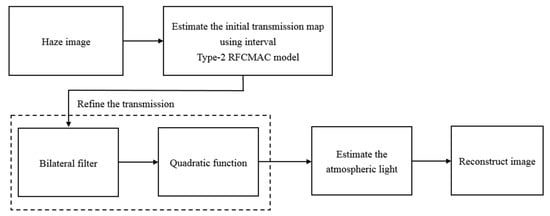
Figure 1.
Flowchart of image dehazing process.
2.1. Initial Transmission Map Estimation Using IT2RFCMAC Model
This section discusses the estimation of the initial transmission map in two parts. This study uses the IT2RFCMAC model as a learning architecture, which acts as trainer and estimator. First, the IT2RFCMAC model and dynamic group artificial bee colony are used for training data. The idea of training data is from the principle of dark channel prior mentioned in []. At least one color channel of the three color channels in the haze image has the minimum pixel value, which approaches 0. This pixel value is the estimated value of transmission map of the pixel. According to this principle, the haze image is observed, as shown in Figure 2. In Figure 2a, the region with a low minimum pixel value of three channels represents the color with high saturation, i.e., the region free of haze interference; hence, the estimated intensity value of transmission map in Figure 2b approaches 1. On the contrary, the region with a high minimum pixel value of three channels in Figure 2a represents the region with haze or cloud layer, meaning the color saturation is low. In order to avoid the low saturation of the haze region influencing the full image, the intensity value of the transmission map in Figure 2b will approach 0. According to the above description, the pixel value and transmission map value present inversely proportional linear variation. Therefore, the training data imported into the IT2RFCMAC model are the pixel values of three color channels (R, G, B), and the output is the transmission map value defined accordingly.
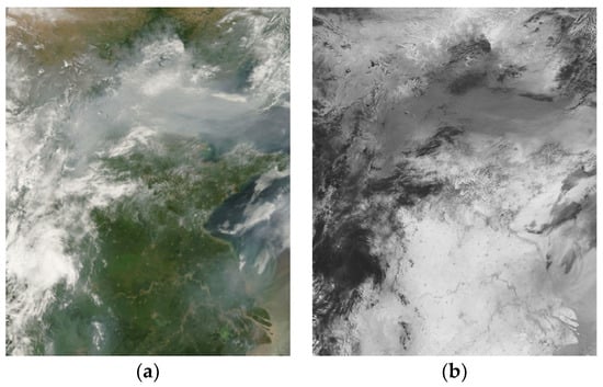
Figure 2.
Schematic diagram of (a) Original haze image; (b) Estimated transmission map.
Figure 3 is the processing flow chart of estimating the initial transmission map proposed in this study. First, one haze satellite image is imported. The 7 × 7 patch size scanning moves one pixel at a time, and the individual minimum pixel values of R, G, B channels of the patch are extracted. Afterwards, the three (R, G, B) minimum pixel values are used as the input variables of the IT2RFCMAC model, the initial transmission map of the image is estimated by such a learned controller output.
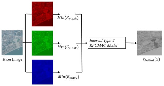
Figure 3.
Initial transmission map estimation using the IT2RFCMAC model.
2.1.1. The Proposed Interval type-2 RFCMAC Model
The neural network and fuzzy theory have become a popular research subject and have been proved applicable to many fields, such as image processing, control, and recognition. The cerebellar model articulation controller (CMAC) [] is inspired by the conception of an artificial neural network (ANN) composed of a multilayer network architecture. The CMAC imitates the operation of the human cerebellum, which is characterized by fast learning, good local generalization capability, and easily implemented architecture. The CMAC has been used in many fields [,]; however, the CMAC needs large amounts of memory space for high dimension problems, and its ability for approximation of function is relatively poor. In order to enhance the search capability of CMAC, many scholars proposed some methods to remedy the deficiencies in the cerebellar model, such as improved controllers as the hierarchical fuzzy cerebellar model articulation controller (Hierarchical Fuzzy CMAC) [], fuzzy cerebellar model articulation controller (FCMAC) [], and recurrent cerebellar model articulation controller (Recurrent CMAC) [,,]. Wang et al. [] proposed a recurrent fuzzy cerebellar model articulation controller (RFCMAC) for solving single-image visibility in a degraded image.
This section introduces the IT2RFCMAC model proposed in this paper. The IT2RFCMAC model is combined with the interval type-2 fuzzy set, FCMAC model, and recurrent memory method to improve the conventional CMAC, as shown in Figure 4. The linear combination of input variables is used as the consequence of the fuzzy hypercube (Takagi–Sugeno–Kang function, TSK function), implementing the rule of fuzzy IF-THEN:
where represents the fuzzy hypercube (i.e., fuzzy rule), represents the input, represents the membership function of the input resulted from the fuzzy hypercube, y represents the consequent output resulted from TSK-function, represents the weight of the fuzzy hypercube in the consequent part, represents the weight in the fuzzy hypercube of the input in the consequent part.
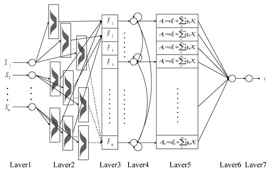
Figure 4.
Architecture diagram of the Interval Type-2 Recurrent Fuzzy Cerebellar Model Articulation Controller (IT2RFCMAC) model.
- Layer 1 (Input layer): This layer receives the input of data in the network architecture, expressed as Equation (3):where represents the number of inputs.
- Layer 2 (Fuzzification layer): This layer converts the input crisp value of layer 1 into fuzzy linguistic information, i.e., fuzzification operation. Each block of the layer is defined as interval type-2 fuzzy sets, as shown in Figure 5. The Gaussian membership function is composed of uncertain mean and a fixed variance . The Gaussian membership function of the interval type-2 fuzzy sets is defined as follows:where and represent the center point and width of the Gaussian membership function of the input, respectively. The footprint of uncertainty is created by parallel translation of the grade of membership of the Gaussian membership function , expressed as upper membership function and lower membership function , defined as follows:and
 Figure 5. Interval type-2 fuzzy sets.
 - Therefore, the output of each block in layer 2 is an interval of .
- Layer 3 (Firing layer): Each node of this layer gathers together to form the fuzzy hypercube according to the grade of membership of each rule of layer 2, mapping to each node of layer 3. The firing strength of each hypercube of this layer is obtained by algebraic product operation,wherewhere and are the upper and lower firing strengths of each hypercube, respectively. M is the hypercube number.
- Layer 4 (Recurrent layer): The output of this layer is composed of current firing strength and previous output of all fuzzy hypercubes, this architecture endues the model with internal memory capacity, expressed as follows:wherewhere and are the recurrent weight of previous and current rule firing strengths, respectively, M is the total number of rules (hypercube), the recurrent weight is the random number of [0,1], the total number is , and and represent the previous output of .
- Layer 5 (Consequent layer): This layer obtains the output of layer 5 from the input of layer 1 by linear equation, i.e., the Takagi–Sugeno–Kang function (TSK function), so as to replace the traditional logic inference process.Wherewhere represent constants.Layer 6 (Defuzzification layer): This layer equates each node of layer 5 with each memory of CMAC, mapping the output fuzzy hypercube of layer 4 to the corresponding memory to form fuzzy output. Afterwards, type-1 fuzzy set is generated by type-reduction operation of interval type-2 fuzzy system using type-reduction []. Finally, the output of crisp value obtained by centroid defuzzification is .
- Layer 7 (Output layer): This layer calculates the mean of output of layer 6 for defuzzification. The output of the final crisp value is obtained as follows:
2.1.2. The Proposed Dynamic Group Artificial Bee Colony
The conventional artificial bee colony (ABC) algorithm [] has fast convergence behavior, but it is early to fall into the local optimal solution. Therefore, this study proposes the concept of dynamic group, considering the balance of global search and local search, and the algorithm efficiency is increased. First, all of food sources are ordered according to the fitness, and the best food source is used as the leader employed bees of the first group, the similarity and difference between the other ungrouped food sources and the leader are calculated. The food source more similar to the current leader will be distributed to the current group, playing the role of onlooker bees. When all food sources are grouped, the bees do their own jobs. The proposed dynamic group artificial bee colony (DGABC) algorithm is shown in Figure 6. The processing procedure is described below.
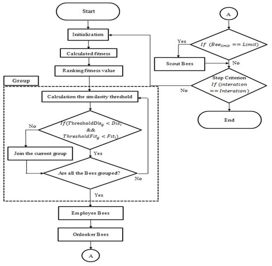
Figure 6.
Flowchart of the proposed dynamic group artificial bee colony (ABC).
Step1 (initialization):
All parameters of the IT2RFCMAC model are coded as a bee, i.e., each bee represents an IT2RFCMAC model. Each fuzzy hypercube dimension contains Gaussian , standard deviation , displacement of interval type-2, and weights and of consequent linear equation, as well as the weight in the recurrent layer (layer 4). The individual bee coding is shown in Figure 7:
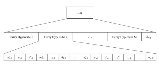
Figure 7.
Schematic diagram of individual bee coding.
Step 2 (ordering):
When the fitness of each bee is calculated, the fitness is ordered from the best to the worst, and all bee group numbers are initialized to 0, as shown in Figure 8:
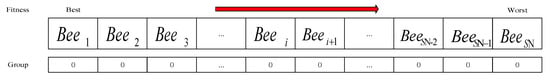
Figure 8.
Schematic diagram of bee colony fitness ordering.
Step3 (grouping):
When the fitness ordering is done, the bee with the best fitness for the moment is taken as the leader of the new group, and the group number is updated. Afterwards, the present leader is taken as group center to define the similarity threshold of the group according to the ungrouped bees, meaning the difference between the bees of the 0th group and the threshold distance and threshold fitness of the current leader is two thresholds. The threshold distance and the threshold fitness difference are expressed as follows:
where is the total number of bees, is the bees of the 0th group among all bee groups, is the dimension, is the position of leader of the group at present, and is the distance threshold of group. is the position of ungrouped bee.
where is the best fitness of leader of group and is the fitness threshold of group.
The ungrouped bee with the best fitness is set as leader and shown in Figure 9:
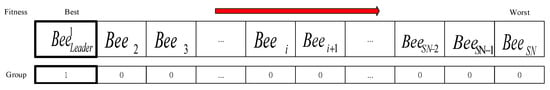
Figure 9.
The bee with the best fitness is set as leader.
The ungrouped bees are calculated again, i.e., the distance difference () and fitness difference () between the bees of the 0th group and current leader, and whether the ungrouped bees are of the group is judged according to the aforesaid thresholds. The distance difference is expressed as follows:
If and , the bee is very similar to the current leader, and the bee is classified into the group of current leader, and the group number is updated as current group number. The bees mismatching the condition will not be classified into the group, as shown in Figure 10:
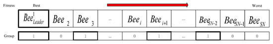
Figure 10.
Similar bees are put in the same group.
If there are bees not yet grouped, the bee with the best fitness is selected from the ungrouped bees in step 3 as the leader of a new group. The grouping actions are repeated until all ungrouped bees are grouped. As shown in Figure 11:
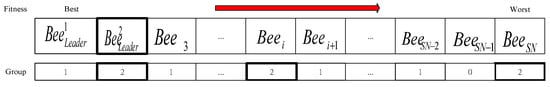
Figure 11.
Group the ungrouped bees.
Step 4 (bee movement):
When all the bees are grouped, the bee move search is implemented to find the best food source. In order to increase the efficiency of the algorithm, the traditional move mode of employed bees is improved in this study; hence, the information of optimal solution is added to the global search of employed bees. On the one hand, the employed bees advance towards the best food source. On the other hand, the random search mechanism of conventional ABC is maintained, so as to avoid too fast algorithm convergence which can easily to fall into the local solution. The improved employed bees search is expressed as follows:
where and are random numbers within , is the position of the employed bee with the best fitness among all employed bees groups, is the position of the employed bee selected randomly from all employed bees groups.
The strategy of dynamic group is added to the local search stage of onlooker bees. Therefore, the group leader (employed bees) must lead the onlooker bees to implement a group search, the original exploration of onlooker bees is improved to refer to the direction of their group leader. The improved search is expressed as follows:
where is the random number within and is the position of the group leader.
2.2. Transmission Map Refinement Using Bilateral Filter and Quadratic Function
The aforesaid halo and color oversaturation resulted from using IT2RFCMAC model to estimate the transmission map are solved by using a bilateral filter and quadratic function.
2.2.1. Bilateral Filter
In order to inhibit the halo effect on the image, this study uses a smooth filter based on image edge preservation and noise abatement, known as a bilateral filter []. The bilateral filter considers the distance and intensity values of two pixels, known as spatial domain and intensity domain of image, respectively. Therefore, the transmission map estimated by the IT2RFCMAC model is used as the intensity value of pixel in the image. The initial transmission map is used as the target image for bilateral filter processing, and the weights of the center for peripheral pixels are calculated by the following equation:
where is the weight of the spatial domain. The closer the adjacent pixel is to the center pixel , the higher is the weight obtained. On the contrary, the farther the adjacent pixel is to the center pixel , the lower is the weight obtained. represents the patch center coordinate. represents the coordinate of pixel around patch center pixel. is the parameter for adjusting the Gaussian weight in the spatial domain; the larger the value is, the more blurred is the image. is set as 10 in this study. represents the Euclidean distance between two pixels in the spatial domain, also known as Euclidean distance.
where is the weight of the intensity domain. The smaller the brightness difference between adjacent pixel and center pixel , the higher is the weight obtained. On the contrary, the larger the brightness difference between adjacent pixel and center pixel , the lower is the weight obtained. represents the intensity value of patch center pixel. represents the intensity value of pixel around patch center. is the parameter for adjusting the Gaussian weight in the intensity domain; is set as 5 in this study. represents the Euclidean distance between two pixels in the intensity domain.
Afterwards, the weight of the spatial domain and the weight of the intensity domain are integrated and multiplied by the transmission map value of the patch center adjacent pixel and normalized. The inhibition of halo of in the initial transmission map by bilateral filter is obtained, expressed as follows:
where represents the patch used.
Figure 12a shows the halo phenomenon resulted from the estimated initial transmission map, mostly distributed over the vehicle and building edges. Figure 12b shows the halo smoothing effect of the bilateral filter in this study.
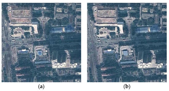
Figure 12.
The halo phenomenon result. (a) Halo image; (b) image after bilateral filter.
2.2.2. Quadratic Function
When the halo is inhibited by bilateral filter, there is still color over saturation in some reconstructed images. Therefore, this study proposes a quadratic function nonlinear conversion to refine the linear transmission map, expressed as follows:
where is the transmission map processed by bilateral filter; the coefficients a and b adjust the curvature of the curve, set as 0.14 and 0.71, respectively. The value of the coefficient is compensated according to the gray level mean of the full image. is set as 0.14 in this study. According to the transmission map function curve in Figure 13, the horizontal axis is the referenced transmission map intensity , and the vertical axis is to refine the intensity value according to the corresponding horizontal axis intensity value. First, the horizontal axis transmission map intensity value approaches 0 in Figure 13, equivalent to thick haze, cloud layer, and white object regions in the image. This viewpoint can be obtained from Equation (1). The value in Equation (26) is used to increase the value of the curve approaching 0. The purpose is to keep some haze particles in the image, so that the image looks more natural. Secondly, the increase of the horizontal axis intensity value in Figure 13 controls a very important part from haze to haze-free intervals. It is observed that using a linear method to refine the transmission map cannot overcome the color oversaturation effectively. Therefore, the purpose of using the nonlinear quadratic function curve to refine the transmission map is to make the variation of transmission map more flexible; i.e., in Equation (26), adjustment of smoothness of the overall curve by coefficients . Finally, the region where the horizontal axis transmission map intensity value approximates 1 is a region of the real image, so the transmission map is free of refined adjustment.
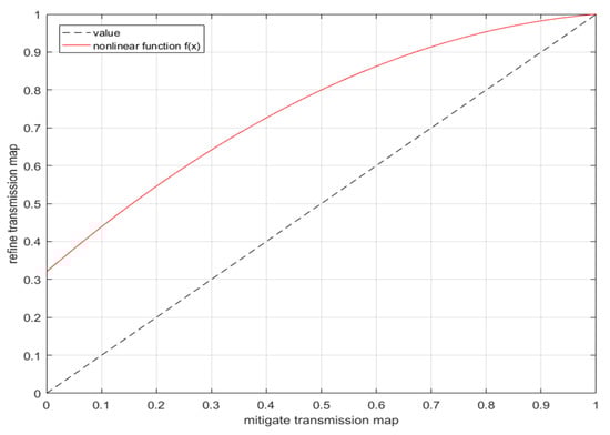
Figure 13.
Nonlinear conversion function.
2.3. Estimation of Atmospheric Light
The atmospheric light is mainly from the light scattered by the atmospheric particles. It is observed in the haze model in Equation (1) that in the overall image reconstruction process, the effect of atmospheric light is a very important factor. According to Equation (1), if the value of the transmission map approaches 0, the haze image is equal to the color vector of the atmospheric light. According to this inference, the white region, cloud layer, and haze in the image can be the reference for atmospheric light estimation. However, it is found in the experiment that if the estimated atmospheric light value is too large or too small, the image after dehazing may be too dark or too bright; therefore, it is a big challenge to estimate the atmospheric light exactly in the haze image. The common method obtains atmospheric light referring to the method of He et al. []. The authors extract the first of bright pixels from the image processed by the dark channel prior as the color vector of atmospheric light. Such a practice may obtain the color vector of atmospheric light accurately for satellite images, but it is found in the experiment that the first of atmospheric light values of a haze satellite image are quite large. Thus, the image becomes quite dark.
After several times of experimental adjustment, the first 1% of atmospheric light is selected as the atmospheric light color vector, as shown in Figure 14. First, the minimum pixel value of three color channels is extracted from each pixel of image, and the first bright pixels are extracted from the maximum to minimum pixel values, the pixels correspond to the pixel position in the original haze satellite image. The three-channel pixel values in the pixel position are added up and divided by 1% of pixels to obtain the final atmospheric light color vector. The virtual codes of the atmospheric light estimation method are shown in Algorithm 1.
| Algorithm1 Atmospheric light estimation algorithm |
| Igray(x)=min(Ic(x)); |
| Counter=(Width of image)*(Height of image)*1%; |
| for(Pixel value descending from 255 to 0) |
| for(width of image) |
| for(Height of image) |
| if(Igray(x) == Current index of pixel value) |
| Pixelc(x) += Ic(x); |
| Counter - -; |
| end if |
| end for |
| end for |
| end for |
| ; |
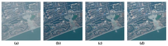
Figure 14.
Comparison diagram of restored images with different proportions of atmospheric light values. (a) Original haze satellite image; (b) The first 0.1% of bright atmospheric light; (c) The first 1% of bright atmospheric light; (d) The first 10% of bright atmospheric light.
2.4. Restored Image
The refined transmission map is obtained by using the aforesaid bilateral filter and quadratic function, so as to overcome the halo and color oversaturation problems, and the atmospheric light color vector is estimated. The refined transmission map and atmospheric light are used as parameters of the reconstructed image. The reconstructed image is expressed as follows:
where is the refined transmission map, and is the estimated atmospheric light color vector.
3. Experimental Results
This section indicates that the parameters used in the IT2RFCMAC model for this study include the total number of bee groups, limited scout bees, generation number, and number of hypercubes, as shown in Table 1. The learning curve between the conventional ABC and improved ABC in training process is analyzed, as shown in Figure 15.

Table 1.
The parameters of Interval Type-2 RFCMAC Model.
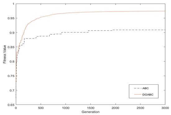
Figure 15.
Learning curves of the conventional ABC and the proposed dynamic group artificial bee colony (DGABC).
It is difficult to adjust the number of hypercubes in the IT2RFCMAC model; therefore, this study uses 4, 6, and 8 hypercubes, respectively, and implements 10 cross validations, respectively. The results are shown in Table 2. The fitness is calculated as follows:
where RMSE represents the root mean square error value.
Table 2.
Benefits of different hypercubes.
According to the results in Table 2, using 4 hypercubes costs less memory space and shorter training time; however, the performance is not good. Using 8 hypercubes consumes more memory space and longer computing time, but the performance is better than using 4 hypercubes. However, according to the best solution, this study adopts 6 hypercubes in the IT2RFCMAC model.
It is observed in Figure 15 that the conventional ABC algorithm falls into the region solution due to the fast convergence of learning. The proposed DGABC algorithm in this study can find the optimal solution effectively by improving the employed bees’ global searching ability and onlooker bees’ local searching ability in the learning curve diagram.
After the aforesaid module architecture and algorithm parameter analysis, the results of the proposed method will be presented by using the experimental images, including hazy satellite images from the Internet and NASA. People are subjective in image observation; hence, it is difficult to define better image quality. For this problem, this study uses two evaluation methods, which are visual assessment and quantitative evaluation, and compared them with the methods proposed by He et al. [], Long et al. [], Wang et al. [], Pan et al. [], and Wei et al. [].
3.1. Visual Assessment
Figure 16 shows the visual assessment methods with respect to the original haze image, the state-of-the-art methods of [,,,,], and the proposed method. For the images in Figure 16b,e, we used a guided filter to filter the halo of edges for dehazing. The effect is obvious; the region covered with haze can be removed, and the processed image is much brighter. However, a halo effect remains on the edges, e.g., the mountain edge. The image results by Long et al. [], as shown in Figure 16c, show oversaturation, because the authors used a single patch size to estimate the transmission map. For the processed results in Figure 16d, the dehazing effect on the haze region is good due to fuzzy control for estimating the transmission map and weight strategy for overcoming the halo problem. However, the whole image has visually severe color oversaturation. Wei et al. [] used linear conversion to adjust the estimated initial transmission map in the processing procedure; however, the light attenuation is a nonlinear problem. The adjustment of the transmission map is difficult to make be flexible which caused the poor performance of the brightness enhancement procedure after dehazing. The processed image, as shown in Figure 16f, was much brighter, the visual effect was unnatural, and the image lost many object colors. Last, in Figure 16g, the color contrast of the proposed method is much better than the other methods. Furthermore, the information covered with haze can be presented in the haze region, and the haze-free region preserves the original colors of the image.
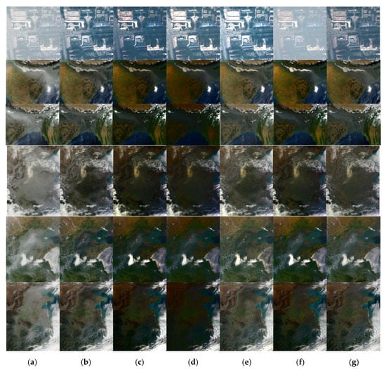
Figure 16.
Comparison of visual assessment. (a) Original haze image, (b) He et al. [], (c) Long et al. [], (d) Wang et al. [], (e) Pan et al. [], (f) Wei et al. [], (g) proposed method.
3.2. Quantitative Evaluation
This section uses and , two quantitative indexes proposed by Hautiere et al. [], to evaluate the image visibility and detail after dehazing. The index evaluates the visibility ratio of the reconstructed image edge which is expressed as Equation (29):
where is the total number of visible edges in the dehazing image. is the total number of visible edges in the original image.
Secondly, index represents the geometric mean rations of the gradient norms of the image’s visible edge before and after dehazing. The gradient value of the reconstructed image is obtained by using the patch method, and the index is expressed as follows:
where parameter is the element of the corresponding set . represents the set of visible edges in the reconstructed image, is the gradient ratio of the reconstructed image to the original haze image.
Based on these two indices, the comparison results of the aforementioned approaches are revealed in Table 3 and Table 4. The aim is to inhibit the halo, increase the contrast without saturating so that the visual information will not be lost. The good results are described by high values of and . Long et al. [] and Wang et al. [] had color oversaturation in the visual assessment after image dehazing; hence, the value of index is much higher than those of other methods. He et al. [] and Pan et al. [] used a guided filter to inhibit the halo, and the image edge details remained. Therefore, the index had good results, but the visual assessment had the halo phenomenon. Comparatively, the proposed method successfully constrains the halo effect and retains the detail of the image edges. Moreover, the image color of the proposed method does not occur the oversaturation phenomenon.
Table 3.
Comparison results of using various methods.
Table 4.
Comparison results of using various methods.
3.3. Discussion
Owing to the purposes of the remote sensing satellite image, such as obtaining information related to the Earth’s resources or monitoring the environment of the Earth’s surface, the images should be processed accurately and transmitted instantly. The comparison results of the average image processing time using various methods are displayed in Table 5. In Table 5, a guide filter algorithm is able to reduce time complexity. However, both He et al. [] and Pan et al. [] reach longer processing times than other methods. Long et al. [] and Wei et al. [] use a single patch to estimate the transmission map which is the fastest in comparison. The proposed method uses the IT2RFCMAC model to estimate the transmission map, and then subsequently applies a bilateral filter to refine the transmission map. Although it costs more time, the reconstructed image shows superior results. The processing speed of the proposed method is not able to be implemented in a real-time system. Therefore, to achieve high-speed operation in real-time applications, the proposed method will be implemented on a field programmable gate array (FPGA), and several image transmission compression technologies [,] will be also considered.
Table 5.
Comparison results of the average image processing time using various methods.
After visual assessment and quantitative evaluation, the advantages and disadvantages using various methods are provided in Table 6. He et al. [] and Pan et al. [] maintain good image edge details, which means those methods can inhibit a halo successfully. However, because the image processing time is long in [] and [], both methods are hard to implement in real-time systems. Long et al. [] and Wang et al. [] have color oversaturation issues, which make an image look untrue. The proposed method is able to inhibit halo, and the color is not saturated; the image processing time is also acceptable.
Table 6.
The advantages and disadvantages using various methods.
4. Conclusions
This study proposes a dehazing method for satellite images. The approach estimates the initial transmission map by interval type-2 RFCMAC (IT2RFCMAC) model. The IT2RFCMAC model is treated as a trainer and estimator. The proposed dynamic group artificial bee colony is used to train the learning parameters of the IT2RFCMAC model. Subsequently, to inhibit the halo and color oversaturation after haze processing, the transmission map is refined by bilateral filter and quadratic function. Afterwards, the first 1% of bright pixels are used as the color vector of atmospheric light. Finally, the refined transmission map and atmospheric light are integrated into the reconstructed image. In the experimental results, the constructed image implemented by the proposed approach shows less haze, less halo, and better color balance than those of other methods.
In future works, the proposed method will be implemented on an FPGA for solving the time-consuming task of image processing, and the image compression for reducing the transmission time will be also considered.
Author Contributions
Conceptualization, C.-J.L. and S.-H.W.; methodology, C.-J.L., C.-H.L. and S.-H.W.; software, C.-J.L. and C.-H.L.; data curation, C.-H.L.; writing—original draft preparation, C.-J.L. and C.-H.L.; writing—review and editing, C.-J.L. and C.-H.L.; funding acquisition, C.-J.L. All authors have read and agreed to the published version of the manuscript.
Funding
This research was funded by the Ministry of Science and Technology of the Republic of China, grant number MOST 108-2221-E-167-026.
Acknowledgments
The authors would like to thank the Ministry of Science and Technology of the Republic of China, Taiwan for financially supporting this research under Contract No. MOST 108-2221-E-167-026.
Conflicts of Interest
The authors declare no conflict of interest.
References
- Lang, F.; Yang, J.; Yan, S.; Qin, F. Superpixel segmentation of polarimetric synthetic aperture radar (SAR) images based on generalized mean shift. Remote Sens. 2018, 10, 1592. [Google Scholar] [CrossRef]
- Ciecholewski, M. River channel segmentation in polarimetric SAR images: Watershed transform combined with average contrast maximisation. Expert Syst. Appl. 2017, 82, 196–215. [Google Scholar] [CrossRef]
- Braga, A.M.; Marques, R.C.P.; Rodrigues, F.A.A.; Medeiros, F.N.S. A Median regularized level set for hierarchical segmentation of SAR images. IEEE Geosci. Remote Sens. Lett. 2017, 14, 1171–1175. [Google Scholar] [CrossRef]
- Jin, R.; Yin, J.; Zhou, W.; Yang, J. Level set segmentation algorithm for high-resolution polarimetric SAR images based on a heterogeneous clutter model. IEEE J. Sel. Top. Appl. Earth Obs. Remote Sens. 2017, 10, 4565–4579. [Google Scholar] [CrossRef]
- Fattal, R. Single image dehazing. ACM Trans. Graph. 2008, 27, 1–9. [Google Scholar] [CrossRef]
- Tan, R.T. Visibility in bad weather from a single image. In Proceedings of the 2008 IEEE Conference on Computer Vision and Pattern Recognition, Anchorage, AK, USA, 23–28 June 2008. [Google Scholar] [CrossRef]
- Tarel, J.P.; Hautiere, N. Fast visibility restoration from a single color or gray level image. In Proceedings of the 2009 IEEE 12th International Conference on Computer Vision, Kyoto, Japan, 29 September–2 October 2009. [Google Scholar] [CrossRef]
- He, K.; Sun, J.; Tang, X. Single image haze removal using dark channel prior. IEEE Trans. Pattern Anal. Mach. Intell. 2011, 33, 2341–2353. [Google Scholar] [CrossRef]
- He, K.; Sun, J.; Tang, X. Guided Image Filtering. IEEE Trans. Pattern Anal. Mach. 2013, 35, 1397–1409. [Google Scholar] [CrossRef]
- Shiau, Y.H.; Chen, P.Y.; Yang, H.Y.; Chen, C.H.; Wang, S.S. Weighted haze removal method with halo prevention. J. Vis. Commun. Image Represent. 2014, 25, 445–453. [Google Scholar] [CrossRef]
- Wang, J.G.; Tai, S.C.; Lin, C.J. Image haze removal using a hybrid of fuzzy inference system and weighted estimation. J. Electron. Imaging 2015, 24, 033027. [Google Scholar] [CrossRef]
- Ge, G.; Wei, Z.; Zhao, J. Fast single-image dehazing using linear transformation. Optik 2015, 126, 3245–3252. [Google Scholar] [CrossRef]
- Chen, Y.; Li, Z.; Bhanu, B.; Tang, D.; Peng, Q.; Zhang, Q. Improve transmission by designing filters for image dehazing. In Proceedings of the 2018 IEEE 3rd International Conference on Image, Vision and Computing (ICIVC), Chongqing, China, 27–29 June 2018. [Google Scholar] [CrossRef]
- Ancuti, C.O.; Ancuti, C. Single Image Dehazing by Multi-Scale Fusion. IEEE Trans. Image Process. 2013, 22, 3271–3282. [Google Scholar] [CrossRef]
- Liu, H.B.; Yang, J.; Wu, Z.P.; Zhang, Q.N. Fast single image dehazing based on image fusion. J. Electron. Imaging 2015, 24, 013020. [Google Scholar] [CrossRef]
- Long, J.; Shi, Z.; Tang, W.; Zhang, C. Single remote sensing image dehazing. IEEE Geosci. Remote Sens. Lett. 2014, 11, 59–63. [Google Scholar] [CrossRef]
- Pan, X.; Xie, F.; Jiang, Z.; Yin, J. Haze removal for a single remote sensing image based on deformed haze imaging model. IEEE Signal Process. Lett. 2015, 22, 1806–1810. [Google Scholar] [CrossRef]
- Ni, W.; Gao, X.; Wang, Y. Single satellite image dehazing via linear intensity transformation and local property analysis. Neurocomputing 2016, 175, 25–39. [Google Scholar] [CrossRef]
- Ouahabi, A. A review of wavelet denoising in medical imaging. In Proceedings of the 2013 8th IEEE International Workshop on Systems, Signal Processing and their Applications (WoSSPA), Algiers, Algeria, 12–15 May 2013. [Google Scholar] [CrossRef]
- Ouahabi, A. Signal and image multiresolution analysis; ISTE-Wiley: London, UK, 2012. [Google Scholar]
- Wang, Z.; Hou, G.; Pan, Z.; Wang, G. Single image dehazing and denoising combining dark channel prior and variational models. IET Comput. Vis. 2018, 12, 393–402. [Google Scholar] [CrossRef]
- Albus, J.S. A new approach to manipulator control: the cerebellar model articulation controller (CMAC). J. Dyn. Syst. Meas. Control 1975, 97, 220–227. [Google Scholar] [CrossRef]
- Iiguni, Y. Hierarchical image coding via cerebellar model arithmetic computers. IEEE Trans. Image Process. 1996, 5, 1393–1401. [Google Scholar] [CrossRef] [PubMed]
- Juang, J.G.; Lee, C.L. Applications of cerebellar model articulation controllers to intelligent landing system. J. Univers. Comput. Sci. 2009, 15, 2586–2607. [Google Scholar] [CrossRef]
- Yu, W.; Rodriguez, F.O.; Moreno-Armendariz, M.A. Hierarchical fuzzy CMAC for nonlinear systems modeling. IEEE T Fuzzy Syst. 2008, 16, 1302–1314. [Google Scholar] [CrossRef]
- Chen, J.Y.; Tsai, P.S.; Wong, C.C. Adaptive design of a fuzzy cerebellar model arithmetic controller neural network. IEE Proc. Control Theory Appl. 2005, 152, 133–137. [Google Scholar] [CrossRef]
- Lin, C.M.; Chen, L.Y.; Yeung, D.S. Adaptive filter design using recurrent cerebellar model articulation controller. IEEE Trans. Neural Netw. 2010, 21, 1149–1157. [Google Scholar] [CrossRef] [PubMed]
- Yang, T.C.; Juang, J.G. Application of adaptive type-2 fuzzy CMAC to automatic landing system. In Proceedings of the 2010 International Symposium on Computational Intelligence and Design, Hangzhou, China, 29–31 October 2010. [Google Scholar] [CrossRef]
- Lin, C.M.; Yang, M.S.; Chao, F.; Hu, X.M.; Zhang, J. Adaptive filter design using type-2 fuzzy cerebellar model articulation controller. IEEE Trans. Neural Netw. Learn. Syst. 2016, 27, 2084–2094. [Google Scholar] [CrossRef] [PubMed]
- Wang, J.G.; Tai, S.C.; Lin, C.J. Transmission map estimation of weather-degraded images using a hybrid of recurrent fuzzy cerebellar model articulation controller and weighted strategy. Opt. Eng. 2016, 55, 083104. [Google Scholar] [CrossRef]
- Castillo, O.; Melin, P. A review on the design and optimization of interval type-2 fuzzy controllers. Appl. Soft Comput. 2012, 12, 1267–1278. [Google Scholar] [CrossRef]
- Karaboga, D. An Idea Based on Honey Bee Swarm for Numerical Optimization; Technical Report—TR06, Technical Report; Erciyes University: Kayseri, Türkiye, 2005. [Google Scholar]
- Tomasi, C.; Manduchi, R. Bilateral filtering for gray and color images. In Proceedings of the Sixth International Conference on Computer Vision, Bombay, India, 7 January 1998. [Google Scholar] [CrossRef]
- Hautiere, N.; Tarel, J.P.; Aubert, D.; Dumont, E. Blind contrast enhancement assessment by gradient ratioing at visible edges. Image Anal. Stereol. 2008, 27, 87–95. [Google Scholar] [CrossRef]
- Yu, G.; Vladimirova, T.; Sweeting, M.N. Image compression systems on board satellites. Acta Astronaut. 2009, 64, 988–1005. [Google Scholar] [CrossRef]
- Ferroukhi, M.; Ouahabi, A.; Attari, M.; Habchi, Y.; Taleb-Ahmed, A. Medical video coding based on 2nd-generation wavelets: Performance evaluation. Electronics 2019, 8, 88. [Google Scholar] [CrossRef]
© 2020 by the authors. Licensee MDPI, Basel, Switzerland. This article is an open access article distributed under the terms and conditions of the Creative Commons Attribution (CC BY) license (http://creativecommons.org/licenses/by/4.0/).