Measuring Traffic Volumes Using an Autoencoder with No Need to Tag Images with Labels

Abstract

Almost all vision technologies that are used to measure traffic volume use a two-step procedure that involves tracking and detecting. Object detection algorithms such as YOLO and Fast-RCNN have been successfully applied to detecting vehicles. The tracking of vehicles requires an additional algorithm that can trace the vehicles that appear in a previous video frame to their appearance in a subsequent frame. This two-step algorithm prevails in the field but requires substantial computation resources for training, testing, and evaluation. The present study devised a simpler algorithm based on an autoencoder that requires no labeled data for training. An autoencoder was trained on the pixel intensities of a virtual line placed on images in an unsupervised manner. The last hidden node of the former encoding portion of the autoencoder generates a scalar signal that can be used to judge whether a vehicle is passing. A cycle-consistent generative adversarial network (CycleGAN) was used to transform an original input photo of complex vehicle images and backgrounds into a simple illustration input image that enhances the performance of the autoencoder in judging the presence of a vehicle. The proposed model is much lighter and faster than a YOLO-based model, and accuracy of the proposed model is equivalent to, or better than, a YOLO-based model. In measuring traffic volumes, the proposed approach turned out to be robust in terms of both accuracy and efficiency.

1. Introduction

Detecting traffic volumes is the basis on which traffic management and operation is implemented. For example, traffic signal control is totally dependent on the traffic volumes of each lane group that shares a signal phase. Measuring traffic volumes in real time is inevitable for a signal controller to adaptively assign signal phases to each lane group. Traffic volumes also determine the service level of a highway segment with respect to congestion management. For the purpose of transportation planning, an analyst depends on historical traffic volumes collected on an area-wide scale over a long-term basis to decide how best to budget for transportation infrastructure. A conventional spot detector, however, has limitations in accuracy and maintainability when implementing the aforementioned tasks. Although loop detectors are pervasive in current traffic surveillance [1,2], they cannot be a future option due to frequent breakdowns that entail large maintenance costs.

Traffic management centers that depend on probe vehicles also cannot measure traffic volumes and focus on collecting information on traffic speeds or travel times. The present study proposed a robust approach to constantly measure traffic volumes on an area-wide scale. Recently, computer vision technologies have replaced the spot-detecting and probe-based schemes, because high-resolution cameras are now more affordable and deep learning algorithms are easily accessible to engineers for use in processing images.

Prior to the success of deep learning, many rule-based algorithms had been developed to recognize vehicles within an image. The rule-based algorithms can be broken down into three categories according to taxonomy [3]. The first category uses the temporal difference method to capture moving objects by utilizing the differences in two consecutive images [4,5]. The performance of this method is largely affected by unexpected noises such as illumination drift due to changes in weather and to variations in the moving speed of objects. The second category involves use of the optical flow method to recognize moving vehicles from video frames by tracking changes in pixel intensities [6,7,8,9]. With this method, motion vectors of moving vehicles are mathematically derived from changes in pixel intensities. This method is also vulnerable when unexpected noise occurs and adds a computational burden to derive the motion vectors. The last category is background subtraction, which had been the most popular method before learning-based algorithms evolved [10,11]. This method utilizes the difference between a target image and the background image to recognize vehicles. Securing a consistent background image is a decisive factor in the success of this method. Some researchers adopted a dynamic background to avoid the impact of environmental changes by considering local features and motion histograms [12]. Even after obtaining a silhouette image from the background subtraction, a robust algorithm is necessary to recognize vehicles from the blob image. Two different approaches are available: Utilization of the convex hull theory [13] and devising an edge detector [14].

It should be noted that all these methods are rule-based rather than learning-based. This means that their models cannot evolve even when more image data are available. Recently, deep-learning algorithms such as YOLO v3 [15] and Fast-RCNN [16] scored a breakthrough in detecting objects within an image and have been successfully utilized in vehicle counting [17,18,19]. It is likely that learning-based algorithms will soon replace rule-based algorithms for traffic surveillance, since they incorporate advantages in both accuracy and maintainability. Such learning-based algorithms for vehicle detection, however, cannot accomplish the task of measuring traffic volumes. Traffic volume is defined as the number of vehicles passing a cross section of a road segment during a specified period such as 15 min or 1 h. It is necessary to track vehicles across time by continuously matching a vehicle detected in the previous video frame with that in the next frame. A standard Kalman filter, which assumes a constant velocity motion for the state equation and a linear relationship for the observation equation, has been adapted to track vehicles detected by YOLO [20]. The state vector is composed of the center coordinates, the height, the aspect ratio of a bounding box, and their velocities. The first three elements of the state vector are derived from direct observations of the vehicle state. The Kalman filter uses observations to iteratively predict and update the state vector.

Several algorithms are used to match the vehicle state forecasted by a Kalman filter with a corresponding observation in the next time frame. This matching problem can be solved via the Hungarian algorithm that uses the intersection over union (IOU) index [21]. Although the two-step approach succeeded in yielding a robust measurement performance, a simpler and lighter model must be developed.

Although a YOLO can be a robust vehicle detector, it requires a large computing resource for a field implementation. Furthermore, YOLO requires additional training whenever the testbed changes. Drawing a bounding box for every vehicle in training images entails considerable human effort, but it is required in order to accurately recognize vehicles in photos taken from different viewpoints [22].

In the present study, we devised an autoencoder model that would overcome the drawbacks of learning-based traffic volume counters. The proposed model requires neither human input to annotate images nor an additional algorithm to track vehicles after detection. The proposed model was trained in an unsupervised manner and thus eliminates the human effort needed to tag images with labels. In addition, the model is much lighter than any other learning-based models that are used to detect and track vehicles, because it utilizes only a small number of pixels within an image, which corresponds to a virtual cross line drawn on a road segment. The pixel intensities on the virtual line constitute a one-dimensional input vector, and the vector feeds an autoencoder as input and simultaneously becomes a label for the corresponding output. An autoencoder consists of two functional parts. While the former encoding part abstracts an input vector into features of a smaller dimension, the latter decoding part reproduces the original input vector from the abstracted features. Both parts have a generally symmetrical structure. The encoding part of the present model reduces the input vector into a scalar signal. After training, an autoencoder evaluated the signal from an input vector, and a simple rule was adopted to judge the presence of a vehicle. The latter decoding part is used only in the training stage to learn the parameters of an autoencoder.

As with other image-based object detection models, however, this autoencoder model was not immune to the impact of shadows and various illuminations. Furthermore, real vehicle images assume complex patterns, and thus signals representing the same vehicle are not consistent according to which part of a vehicle passes the detection line. Due to these complications, the signals were imperfect in judging whether a vehicle was occupying the virtual line sensor. To tackle the problem, original images were simplified using a CycleGAN developed by [23], so that both vehicles and backgrounds would have monotone colors. Such a transformation had already been successfully adopted in our previous studies measuring traffic speed and delay [22,24].

Section 2 explains how an autoencoder is used to recognize a vehicle’s presence and shows how the model architecture is set up. Section 3 describes how to choose a testbed and collect image data. Section 4 shows how threshold values are selected to judge the vehicle presence and to count the vehicle passages. In the last subsection of Section 4, the traffic volumes measured from the present approach are compared with those from a YOLO+SORT algorithm [18]. Section 5 extends both the proposed model and the reference model, and the results are compared. The first subsection of Section 5 provides a brief description of the CycleGAN that was used to convert real photos into simple images. The following subsections describe how an autoencoder model was trained and tested on the synthesized images, and how a YOLO+SORT algorithm was fine-tuned using additional aerial photos. In Section 5, the efficiency of the proposed model is compared with a reference model and a plausible method to classify vehicle types based on the proposed model introduced. Finally, Section 6 draws conclusions and suggests further studies to develop the present approach.

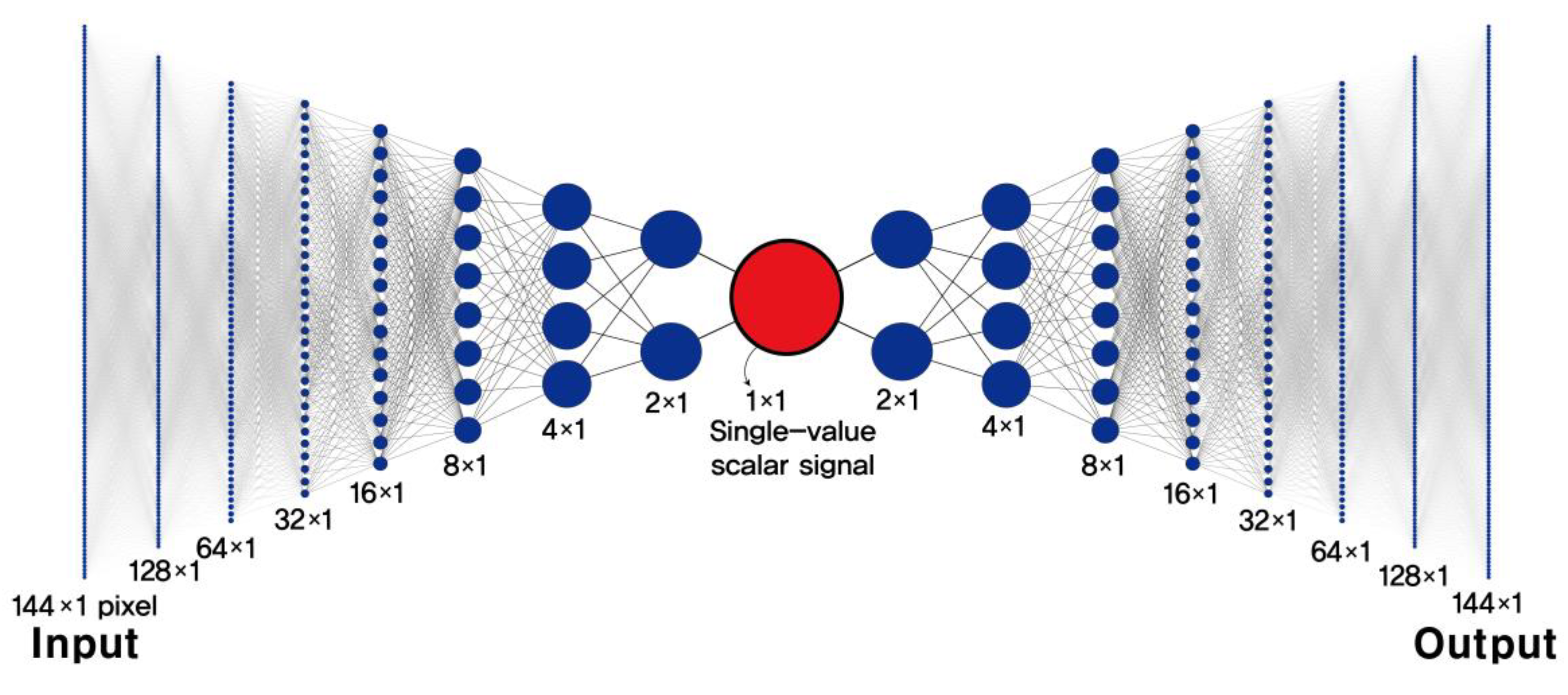
2. An Autoencoder Recognizes the Presence of Vehicles

Autoencoders have been utilized to reduce the dimensions of input features [25,26], to remove the noise from corrupted input data [27,28], and to pretrain the weights of a supervised deep learning model [29,30]. In addition to these typical uses, autoencoders have been used for many other purposes [31]. An autoencoder belongs to the category of unsupervised learning models because it requires no human effort to label or annotate data for training. This is a great advantage of an autoencoder-based model when adapted to measuring traffic volumes. A standard autoencoder was employed in the present study to reduce the dimensions of an input feature into only a scalar signal without supervision. We expected the signal to be fully qualified to recognize the presence of a vehicle.

A cross line drawn on a road segment was assumed to be a virtual detector for counting traffic volumes. The width of the line was set as only a pixel, so that the input and output vectors for an autoencoder could be one-dimensional. Pixel intensities along the line vary according to the presence and absence of vehicles. The proposed approach was devised under the expectation that an autoencoder could recognize such differences in pixel intensities according to the presence or absence of a vehicle. The former encoder portion of the present autoencoder was established to be symmetrical with the latter decoder portion. Both the encoding and decoding portions of the autoencoder are composed of eight hidden layers, respectively. A single hidden node placed in the middle acts as a potential output node that produces a scalar signal to recognize the presence of a vehicle. The latter decoder portion is used only in the training stage.

$$Loss function=E\left[{\left(F\left(X\right)-X\right)}^T· \left(F\left(X\right)-X\right)\right]$$

(1)

The discrepancy between the input and the output was set as the loss function to be minimized when training the autoencoder. The mean square error (MSE) was chosen to be the loss function. In Equation (1), $X$ is a one-dimensional input vector of the autoencoder. In practice, the absolute value of pixel intensities subtracted from those of an empty road are used as input after normalization. $F\left(X\right)$ is the estimated output vector of the autoencoder. A stochastic gradient descent algorithm was used to train the model, and the batch size was 48. Training data were extracted from video frames of 100 min. Ten percent of the training data were randomly chosen to secure the convergence while sidestepping over-fitting.

Once the model training is complete, only the encoder portion computes a signal that can be used to recognize the presence of a vehicle. Dense layers are stacked to build both the encoder and decoder portions. The number of hidden nodes dwindles to 1 through the encoder portion and is then amplified up to the original input dimensions through the decoder portion. Figure 1 shows the entire architecture of the autoencoder adopted in the present study. For brevity, the activation using the rectified linear unit (ReLU) after each hidden layer is omitted in the figure. A scalar node in the middle is activated with a sigmoid function. The model architecture was set up after testing as many plausible alternative structures as possible.

To facilitate the recognition of vehicle presence, the last signal of the encoder is activated by a sigmoid function, such that the signal ranges between 0 and 1. It is likely that the signal for vehicle presence will approach either of the boundary values. However, which value indicates the presence of a vehicle is unknown even after training the autoencoder. To understand the boundary value for vehicle presence, an analyst must intuitively examine the video stream used for training by comparing signal estimates with the vehicle presence. Based on the examination, a threshold value should be manually chosen to determine the presence or absence of vehicles. This engineering judgment could be the only limitation in the proposed approach. Although the threshold value may also vary according to the times of day and the weather conditions, it is difficult in practice to prepare different threshold values in advance. We suggest a revolutionary method in the fourth section to overcome this difficulty by transforming complex real photos into simple illustrations based on a CycleGAN.

3. Testbed and Data Collection

An intersection approach with four lanes was chosen as the testbed to train and test the proposed autoencoder. One hundred minutes of video stream were taken from 35 m above the intersection. Figure 2 shows a snapshot of the video stream. For each critical intersection in the Seoul metropolitan area, a 25–35 m high pole is planted to hang a CCTV for multipurpose surveillance. We assumed that the CCTV could be used for the purpose of traffic surveillance since it provides street photos from a bird’s-eye view. The coverage of the testbed was 13 m wide and 34 m long. The virtual line detector was placed ahead of the stop line to avoid the condition whereby a vehicle would occupy the line during a red signal phase. Another reason to draw a virtual detection line closely to the stop line was because a lane change is not permitted when a vehicle is passing the stop line. Even though our ultimate goal was to measure traffic volumes, an autoencoder simply recognizes the presence or absence of a vehicle on a virtual detection line. How the autoencoder output is used to measure traffic volumes will be described in the next section.

The proposed autoencoder model was trained and tested in a single testbed. Usually, testing results are most accurate when the model was trained in the same environment. It is rational that the proposed autoencoder should be trained for each site, since training the model is not a burdensome task without supervision. Trying to find a universal model that can cover all different locations is unnecessary for the present model. Basically, reducing the model size is more important for a real-time application than finding a heavier universal model with many parameters.

To assess the performance of the autoencoder, vehicle presence was manually identified during the entire time period. That is, the actual presence of vehicles on the virtual detection line was recorded every 0.2 s. Based on the ground truth, the precision and recall for the proposed autoencoder was computed (see the next section).

The present study was focused on confirming whether an autoencoder could be used to measure traffic volumes in the field on a real-time basis. To test the proposed approach, true traffic volumes were observed in the testbed. The number of vehicles passing the virtual detection line of each lane was counted for every two cycles of the traffic signal (=2.5 × 2 min). Based on these data, the final performance of the proposed approach was tested and compared with that of a reference model.

There are two types of object detectors based on deep learning technologies. A Fast-RCNN is accurate but has a disadvantage in computation time because it adopts a two-stage detection algorithm wherein a preprocess of regional proposals precedes a detection task. If a tracking stage is added when measuring traffic volumes, the model should go through three stages, which is not appropriate for a real-time application. On the other hand, a YOLO is a single-stage detection algorithm that has the merit of computation time, which has made the model widely accepted for the real-time recognition of objects. Since traffic volumes should be measured on a real-time basis, instead of the other two-stage models, we adopted a YOLO model as a reference to be compared with the proposed model. As mentioned earlier, the latest YOLO (version 3) with default weights is incapable of detecting vehicles in photos taken from a bird’s-eye view. To fine-tune the YOLO model, we manually drew bounding boxes for all the vehicles in 1500 video frames of the testbed.

4. The Model Performance Based on Real Photos

All analyses in this section are based on real photos from video shoots. First, this section introduces a simple rule-based methodology to choose threshold values used to recognize the presence and absence of vehicles from the signal output of a trained autoencoder. Next, the precision and recall are computed for the autoencoder based on the chosen thresholds. Last, the performance of the proposed approach in measuring traffic volumes is compared with that of a “state-of-the-art” model based on YOLO and SORT [18].

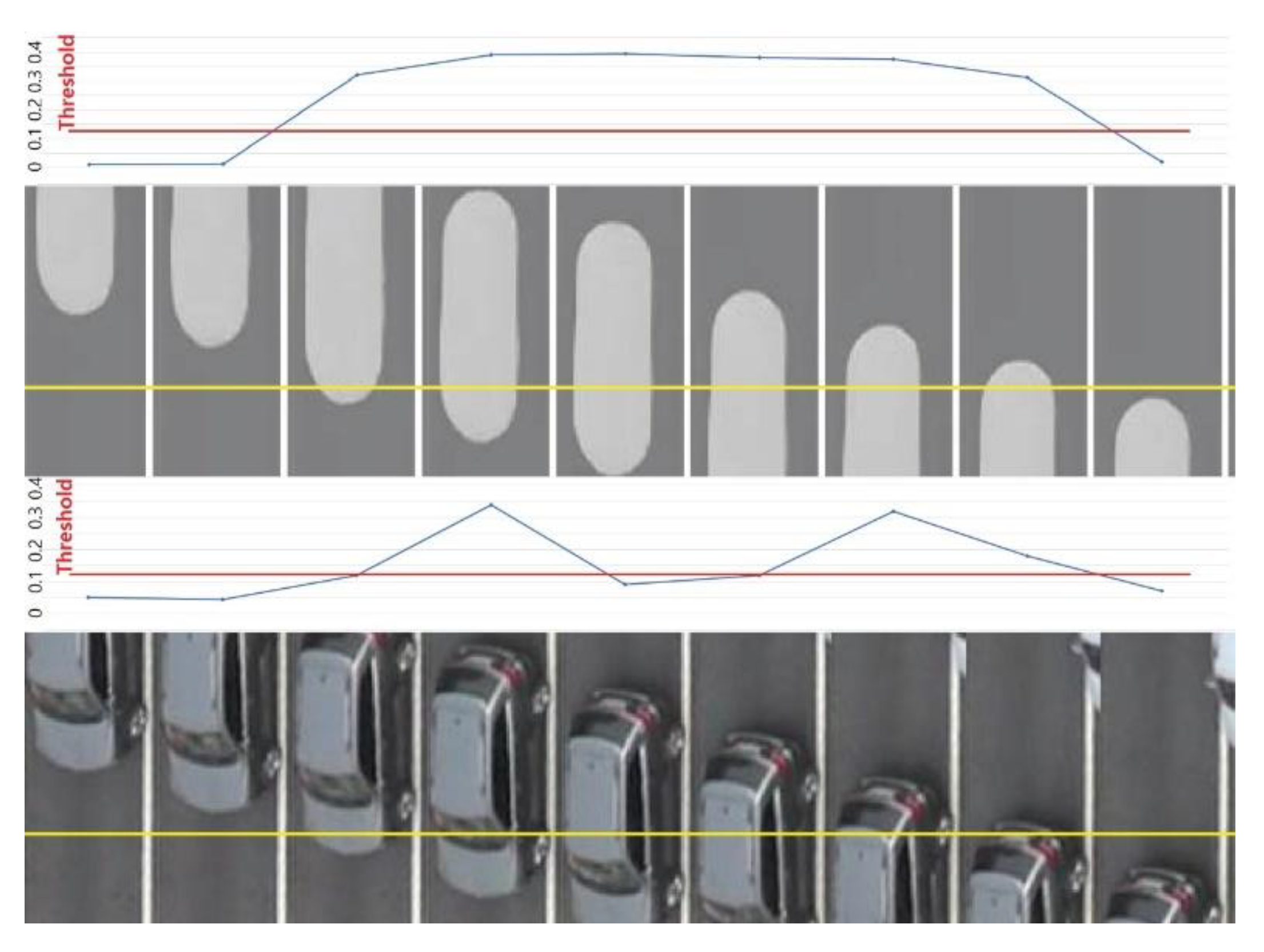
4.1. Choosing Threshold Values to Measure Traffic Volumes

The trained autoencoder provided signals for the test data and the signal profile, as shown in Figure 3. Once a signal profile that a trained autoencoder emits is available, it is possible to find a threshold value with the naked eye by watching the video simultaneously with the signal profile. We selected a threshold value to recognize the presence of vehicles in such a way. When compared with actual video, signal values closer to 1 indicated that a vehicle was occupying the virtual detection line, whereas those closer to 0 corresponded to the background. Unfortunately, there is no rigorous way to drive an optimal boundary between the presence and absence of vehicles. We chose a threshold directly from the signal profile, such that it could be slightly larger than the lowest signal value for the background. The signal value for the background was almost 0, and the chosen threshold was set at 0.06. This manual choice did no harm in recognizing the presence of vehicles, which is verified in the next subsection by computing the precision and recall based on the ground truth.

Although signals are derived from a sigmoid function, 0.5 cannot be selected as a threshold value because the signals corresponding to the presence of vehicles fluctuates significantly. The signal profile in Figure 3 shows variations in the signals of a vehicle’s presence. This fluctuation could have been due to inconsistent shapes and colors of vehicles. If vehicle shapes and colors were consistent, it would be possible to establish a more robust way to choose a threshold value. A CycleGAN [23] will be adopted in the next section to transform real photos into simple illustrations with consistent vehicle shapes and colors.

Once a vehicle’s presence is recognized, the raw signal profile can be updated in a clearer manner, as shown in Figure 4. Another threshold is the necessity to judge whether a series of signals belongs to a vehicle’s passage. It is simple to count vehicles based on the updated signal profile, because the time gap between consecutive vehicles cannot be decreased to a minimum value in an intersection approach. Thus, a period of background shorter than the minimum gap was ignored and incorporated with the previous and next intervals of a vehicle’s presence. The highway capacity manual (HCM, 2020) defines the saturation flowrate in an intersection approach for various geometric and operational conditions. The minimum headway derived from the saturation flowrate under ideal conditions is 1.8 s. This means that no vehicle could pass the stop line within 1.8 s right after the preceding vehicle has passed it. The minimum gap is shorter than the minimum headway according to the time it takes for the vehicle length to pass. The minimum gap (=0.5 s) chosen in the present study was very conservative. This minimum gap is globally applicable. However, the threshold value to recognize the vehicle presence is expected to vary from site to site.

4.2. The Performance of the Autoencoder at Judging the Presence of Vehicles

The precision and recall of the trained autoencoder was computed to evaluate its performance for detecting the presence of vehicles. As mentioned earlier, to validate the autoencoder model we manually recognized the presence of vehicles. To facilitate the labeling task, only the video frames for green signals were utilized. Out of 100-min video frames, 80 min were used for training, and the remainder was reserved for testing.

Table 1. The precision and recall of the proposed autoencoder to identify the presence and absence of vehicles on the virtual detection line.

	Train Data			Test Data
	Positive (Ground Truth)	Negative (Ground Truth)	Sum	Positive (Ground Truth)	Negative (Ground Truth)	Sum
Positive (Predicted)	19,806	456	20,262	4230	84	4314
Negative (Predicted)	1355	51,603	52,958	202	11,164	11,366
Sum	21,161	52,059	73,220	4432	11,248	15,680
Precision	0.977			0.981
Recall	0.936			0.954

shows the precision and recall for both the training and the testing data. Unlike the prior expectation, the testing results were ameliorated somewhat when compared with the training results. This might be due to a coincidence wherein the test dataset includes fewer problematic situations. The test results showed that the proposed autoencoder is not error free. A remedy was needed to increase the model performance, and that will be introduced in the next section.

4.3. The Performance of the Proposed Approach to Measure Traffic Volumes Compared with that of a Yolo-Based Model

The accuracy of measuring traffic volumes for the test data is introduced in this subsection. Since the autoencoder was not perfect in judging the presence of vehicles, its accuracy in measuring the traffic volumes entailed some errors. The traffic volume measured by the autoencoder-based methodology was overestimated when compared with observations. This implies that the methodology mistakenly double-counted some vehicle passages (

Table 2. Comparing the accuracy of the proposed model with that of the reference model.

Accuracy Comparison		Autoencoder Model				YOLO v3 Model
		Lane 1	Lane 2	Lane 3	Lane 4	Lane 1	Lane 2	Lane 3	Lane 4
C1~2	Predicted/ Ground truth	35/34	31/30	18/18	21/21	22/34	29/30	18/18	20/21
C3~4	Predicted/ Ground truth	39/39	42/40	17/17	19/19	38/39	39/40	14/17	17/19
C5~6	Predicted/ Ground truth	46/44	39/39	22/20	16/16	36/44	38/39	20/20	10/16
C7~8	Predicted/ Ground truth	41/43	45/46	21/20	18/18	31/43	44/46	32/20	13/18
Total	Predicted/ Ground truth	161/160	157/155	78/75	74/74	127/160	150/155	84/75	60/74
	Error (%)	+0.6%	+1.3%	+4%	0%	−20.6%	−3.2%	+12%	−18.9%

).

A YOLO-based model was selected as a reference to validate the proposed model. The reference model adopted a two-step approach that involved detecting and tracking. The YOLO detects vehicles, and then a SORT algorithm tracks them [18]. Table 2 compares the accuracy of both the reference and the proposed methodology. Unexpectedly, the accuracy of the reference model was inferior to that of the proposed model. This resulted from the fact that the original YOLO had been trained only on vehicle images taken from the ground view, whereas testing images were taken from an aerial view. In the next section, the model will be fine-tuned using extra labeled images taken from an aerial view to enhance the performance. A CycleGAN-based remedy will also be used to allow the proposed model to overcome the inaccuracy.

5. The Model Performance Based on Synthesized Images

The dependence on real photos is an aspect of the proposed autoencoder that prevents it from sufficiently recognizing the presence of vehicles. Pixel intensities on the detection line are inconsistent while a vehicle is passing the line, because the shape and color of the vehicle varies. A robust way to change an original photo into a simpler image is introduced in this section under the assumption that the performance of the autoencoder could be enhanced if the shape and color of a vehicle were consistent within an image.

A CycleGAN was used to preprocess input images so that a vehicle image could be simpler and more consistent in both color and shape. It should be noted that a CycleGAN is not a prerequisite for an autoencoder to measure traffic volumes, but instead is an assistant tool to refine input images for the best accuracy.

5.1. The Introduction of a Cycle-Consistent Adversarial Network (CycleGAN)

The use of deep learning technologies in computer vision has recently trended toward the development of generative models to synthesize images [23,32,33]. In the use of these technologies, the approach of Zhu et al. [23] has been noteworthy in that an image in one context can be transformed to its corresponding image in another context. A CycleGAN has been used to change the photos of a summer landscape into those of a winter landscape, female photos into male photos, or satellite images into real physical maps. This capability of a CycleGAN also facilitates traffic surveillance that depends on images. We have already used images synthesized by a CycleGAN to enhance the accuracy of measuring both traffic speeds and delays [22,24]. This scheme was adopted in the present study to obtain images that were more consistent at recognizing the presence of vehicles on the detection line.

A CycleGAN is composed of two types of CNN models that are alternately updated during training. A generator converts images in one context to corresponding images in the other context, whereas a discriminator judges which context an image belongs to. Generators are trained to minimize the discrepancies between the images in one context and the images that are cycled from them. The training of discriminators must address two different objectives. A discriminator judges real photos as true and synthesized images as fake. Adversarial learning, however, attempts to deceive a discriminator so that it cannot discern a cycled image from the original real photo. For details concerning the training of a CycleGAN, readers can refer to previously published studies listed in the references [23,24].

Two separate image sets in different contexts are necessary to train a CycleGAN. In the present study, original photos were taken in the field, and cartoon-like illustrations were obtained from a traffic simulator (VISSIM v5.0, PTV, Karlsruhe, Germany). When training a CycleGAN two image sets do not have to be paired, which is a tremendous advantage. That means that no human effort is required to tag photos with labels in order to train a CycleGAN. The only requirement was traffic simulation that would mimic real traffic conditions. Most traffic simulators provide an animation module to visualize the simulation results. This function facilitates the generation of images that contain vehicles that are consistent in shape and color. Figure 5 shows examples of real photos and their corresponding images that were synthesized using a CycleGAN. The synthesized images include jelly-like vehicle shapes, each of which is represented by a constant color. In the next subsection, the enhancement in the performance of the autoencoder will be examined based on precision and recall.

5.2. Enhancing the Performance of the Autoencoder to Better Judge the Presence of Vehicles

As expected, the performance of the autoencoder to judge the presence of vehicles was considerably improved when synthesized images were used instead of real photos for training and testing (compare Table 1 and

Table 3. The precision and recall of the autoencoder when synthesized images are used as input.

	Train Data			Test Data
	Positive (Ground Truth)	Negative (Ground Truth)	Sum	Positive (Ground Truth)	Negative (Ground Truth)	Sum
Positive (Predicted)	20,051	376	20,427	4206	32	4238
Negative (Predicted)	942	51,851	52,793	213	11,229	11,442
Sum	20,993	52,227	73,220	4419	11,261	15,680
Precision	0.982			0.992
Recall	0.955			0.952

). The profile of raw signals from the enhanced autoencoder is quite different from that of the original autoencoder, which was based on real photos (see Figure 3 and Figure 6). The updated profile more closely approximated the final profile after recognizing vehicle passages based on chosen thresholds (see Figure 6 and Figure 7).

Figure 8 was drawn to directly show the reason for the performance enhancement. The signal of a real vehicle varies while passing the virtual detection line (=yellow line), whereas that of a jelly-type vehicle shape synthesized from a CycleGAN is much more consistent. This confirms that the proposed methodology has a great advantage when directly applied to field operation.

5.3. The Performance of the Updated Autoencoder in Measuring Traffic Volumes Compared with that of a Yolo-Based Model

The performance of the autoencoder to measure traffic volumes was improved considerably when synthesized images were used. The accuracy of the updated autoencoder approached 100%, which is much higher than that of the naive autoencoder trained on real photos (compare Table 2 and

Table 4. The accuracy comparison between the updated model and reference model.

Accuracy Comparison		Autoencoder Model (Updated)				YOLO v3 Model (Fine Tuned)
		Lane 1	Lane 2	Lane 3	Lane 4	Lane 1	Lane 2	Lane 3	Lane 4
C1~2	Predicted/Ground truth	34/34	30/30	18/18	21/21	34/34	20/20	18/18	21/21
C3~4	Predicted/Ground truth	39/39	40/40	17/17	19/19	47/39	40/40	16/17	19/19
C5~6	Predicted/Ground truth	44/44	39/39	20/20	16/16	44/44	39/39	20/20	16/16
C7~8	Predicted/Ground truth	41/43	45/46	20/20	18/18	41/43	45/46	25/20	16/18
Total	Predicted/Ground truth	158/160	154/155	75/75	74/74	166/160	154/155	79/75	72/74
	Error (%)	−1.3%	−0.6%	0%	0%	+3.8%	−0.6%	+5.3%	−2.7%

).

The performance of the updated autoencoder to measure traffic volumes was compared with that of a YOLO-based model. For a fair comparison, a YOLO-based model was also updated with extra labeling data. One thousand and five hundred pictures from an aerial view were annotated with bounding boxes to fine tune the original YOLO v3 model with default weights. This took almost a week with two coding experts hired. Drawing a bounding box for every vehicle within all images is a very labor-intensive task, which makes the use of a YOLO-based model less practical for use in traffic surveillance. The performance of the YOLO-based model after fine tuning was comparable to that of the proposed model (Table 4). It should be noted that the proposed model does not require human effort for the task of labeling. Both the autoencoder and the CycleGAN belong to the category of unsupervised learning.

6. The Model Efficiency and the Potential to Classify Vehicle Types

One of the main purposes of the present study is to develop a lighter model that could be implemented on a real-time basis using edge computing. A one-dimensional input instead of a full image has a great advantage in saving computer memory onsite. The comparison of computing time and memory usage is introduced in

Table 5. The efficiency comparison between the proposed model and reference model.

	Number of Parameters	Evaluation Time per Frame
Autoencoder model	59,361	0.00007 s
CycleGAN + Autoencoder model	9,525,101	0.032 s
YOLO v3 model	61,581,727	0.078 s

. The number of parameters in the proposed model was much smaller than that in a YOLO. The proposed model turned out to be much lighter and faster than a YOLO when recognizing vehicles for a frame. Even when a CycleGAN was used to preprocess an input image, a YOLO did not outperform the proposed model in computing speed.

The proposed model did not include the intrinsic function of classifying vehicle types, whereas other image-based models such as YOLO can easily classify vehicle types. A plausible methodology is proposed to classify vehicle types via a simple rule-based approach. It is possible that the vehicle length could be approximately measured under the assumption that the length would be proportional to the passing time. This assumption has been widely accepted when the vehicle type was estimated based on signals from a conventional loop detector. The moving average of a vehicle’s passage time was dynamically updated and used as a basis on which the vehicle length was determined. If a vehicle passage time is larger than a threshold value, the vehicle is categorized into a group of large trucks or buses (Figure 9). We determined a threshold value to be 1.67-fold of the average of vehicle passage times.

On the other hand, a YOLO has the ability to directly classify vehicle types. We reduced the number of classes of a YOLO model and trained it from scratch using our own labeled images without depending on pretrained parameters. A YOLO version 3 was trained so that it could classify three different types of vehicles such as cars, small vehicles, and large vehicles. Small vehicles include SUVs and small trucks, and large vehicles include buses, large trucks, and trailers. For the comparison with the proposed model with only two classes, cars and small vehicles were categorized into a single group of small vehicles. As shown in

Table 6. The accuracy comparison for classifying vehicle types.

Accuracy Comparison	Autoencoder				CycleGAN + Autoencoder				YOLO v3
	Lane 1	Lane 2	Lane 3	Lane 4	Lane 1	Lane 2	Lane 3	Lane 4	Lane 1	Lane 2	Lane 3	Lane 4
Small Vehicle	152/150	155/155	74/73	71/72	149/150	154/155	73/73	72/72	156/150	154/155	77/73	70/72
Large Vehicle	9/10	2/0	4/2	3/2	9/10	0/0	2/2	2/2	10/10	0/0	2/2	2/2

, the proposed model turned out to be capable of classifying vehicle types, even though the performance was slightly inferior to that of a YOLO.

The motorcycles were excluded in measuring traffic volumes. The passage of a motorcycle left smaller signals than vehicles. These signals of motorcycles could be a cause of false positives. Although a carefully chosen threshold turned out to minimize the errors, rigorous measures should be taken to recognize motorcycles, which will depend on two-dimensional signals in the further study.

7. Conclusions

A novel methodology to measure traffic volumes without supervision was developed in the present study. An autoencoder was trained to recognize the presence of vehicles on a cross section of a roadway based solely on pixel intensities. The proposed methodology requires no human effort to tag images with labels. The performance of the proposed model trained on synthesized images approximated that of a YOLO-based model that was fine-tuned with the extra labeling of images. When considering the human effort required for the labeling task, the proposed methodology seems more promising for use in the field.

The proposed methodology, however, demonstrated a critical drawback wherein vehicle types could not be distinguished. It is possible to approximately classify vehicle types if a constant speed is assumed for all moving vehicles. This assumption is acceptable when the detection line is placed on the stop line of an intersection approach. Speed estimation that depends on spot detectors usually adopts such an assumption. Further study is expected to develop a traffic volume counter that could classify each vehicle type.

References

1. Riedel, T.; Erni, K. Do my loop detectors count correctly? A set of functions for detector plausibility testing. J. Traffic Transp. Eng. (JTTE) 2016, 4, 117–130. [Google Scholar]
2. Meng, C.; Yi, X.; Su, L.; Gao, J.; Zheng, Y. City-wide traffic volume inference with loop detector data and taxi trajectories. In Proceedings of the 25th ACM SIGSPATIAL International Conference on Advances in Geographic Information Systems, Redondo Beach, CA, USA, 7–10 November 2017; pp. 1–10.
3. Ozkurt, C.; Camci, F. Automatic Traffic Density Estimation and Vehicle Classification for Traffic Surveillance System using Neural Networks. Math. Comput. Appl. 2009, 14, 187–196. [Google Scholar] [CrossRef] [Green Version]
4. López, M.T.; Fernández-Caballero, A.; Mira, J.; Delgado, A.E.; Fernández, M.A. Algorithmic lateral inhibition method in dynamic and selective visual attention task: Application to moving objects detection and labeling. Expert Syst. Appl. 2006, 31, 570–594. [Google Scholar] [CrossRef] [Green Version]
5. López, M.T.; Fernández-Caballero, A.; Fernández, M.A.; Mira, J.; Delgado, A.E. Visual Surveillance by Dynamic Visual Attention Method. Pattern Recogn. 2006, 39, 2194–2211. [Google Scholar] [CrossRef] [Green Version]
6. Ji, X.; Wei, Z.; Feng, Y. Effective vehicle detection technique for traffic surveillance systems. J. Vis. Commun. Image Represent. 2006, 17, 647–658. [Google Scholar] [CrossRef]
7. Qimin, X.; Xu, L.; Mingming, W.; Bin, L.; Xianghui, S. A methodology of vehicle speed estimation based on optical flow. In Proceedings of the 2014 IEEE International Conference on Service Operations and Logistics, and Informatics, Qingdao, China, 8–10 October 2014; pp. 33–37. [Google Scholar]
8. Indu, S.; Gupta, M.; Bhattacharyya, A. Vehicle tracking and speed estimation using optical flow method. Int. J. Eng. Sci. Technol. 2011, 3, 429–434. [Google Scholar]
9. Haag, M.; Nagel, H.H. Combination of edge element and optical flow estimates for 3D-model-based vehicle tracking in traffic image sequences. Int. J. Comput. Vis. 1999, 35, 295–319. [Google Scholar] [CrossRef]
10. Zhou, J.; Gao, D.; Zhang, D. Moving vehicle detection for automatic traffic monitoring. IEEE Trans. Veh. Technol. 2007, 56, 51–59. [Google Scholar] [CrossRef] [Green Version]
11. Niu, X. A semi-automatic framework for highway extraction and vehicle detection based on a geometric deformable model. ISPRS J. Photogramm. Remote Sens. 2006, 61, 170–186. [Google Scholar] [CrossRef]
12. Qian, Z.M.; Shi, H.X.; Yang, J.K. Video vehicle detection based on local feature. Adv. Mater. Res. 2011, 186, 56–60. [Google Scholar] [CrossRef]
13. Jayaram, M.A.; Fleyeh, H. Convex hulls in image processing: a scoping review. Am. J. Intell.Syst. 2016, 6, 48–58. [Google Scholar]
14. Zhu, Z.; Xu, G. VISATRAM: A real-time vision system for automatic traffic monitoring. Image Vis. Comput. 2000, 18, 781–794. [Google Scholar] [CrossRef]
15. Redmon, J.; Divvala, S.; Girshick, R.; Farhadi, A. You only look once: Unified, real-time object detection. In Proceedings of the IEEE conference on Computer Vision and Pattern Recognition(CVPR), Las Vegas, NV, USA, 6 June–1 July 2016; pp. 779–788. [Google Scholar]
16. Ren, S.; He, K.; Girshick, R.; Sun, J. Faster r-cnn: Towards real-time object detection with region proposal networks. In Proceedings of the Advances in Neural Information Processing Systems (NIPS), Montreal, QC, Canada, 7–12 December 2015; pp. 91–99. [Google Scholar]
17. Asha, C.S.; Narasimhadhan, A.V. Vehicle counting for traffic management system using YOLO and correlation filter. In Proceedings of the 2018 IEEE International Conference on Electronics, Computing and Communication Technologies (CONECCT), Bangalore, India, 16–17 March 2018; pp. 1–6. [Google Scholar]
18. Lopez, G. Traffic Counter with YOLO and SORT. Available online: https://github.com/guillelopez/python-traffic-counter-with-yolo-and-sort (accessed on 11 December 2018).
19. Sang, J.; Wu, Z.; Guo, P.; Hu, H.; Xiang, H.; Zhang, Q.; Cai, B. An improved YOLOv2 for vehicle detection. Sensors 2018, 18, 4272. [Google Scholar] [CrossRef] [PubMed] [Green Version]
20. Bathija, A.; Sharma, G. Visual Object Detection and Tracking using YOLO and SORT. Int. J. Eng. Res. Technol. (IJERT) 2019, 8, 705–708. [Google Scholar]
21. Wojke, N.; Bewley, A.; Paulus, D. Simple online and realtime tracking with a deep association metric. In Proceedings of the 2017 IEEE International Conference on Image Processing (ICIP), Beijing, China, 17–20 September 2017; pp. 3645–3649. [Google Scholar]
22. Shin, J.; Roh, S.; Sohn, K. Image-Based Learning to Measure the Stopped Delay in an Approach of a Signalized Intersection. IEEE Access 2019, 7, 169888–169898. [Google Scholar] [CrossRef]
23. Zhu, J.Y.; Park, T.; Isola, P.; Efros, A.A. Unpaired image-to-image translation using cycle-consistent adversarial networks. arXiv 2017, arXiv:1703.10593. [Google Scholar]
24. Lee, J.; Roh, S.; Shin, J.; Sohn, K. Image-based learning to measure the space mean speed on a stretch of road without the need to tag images with labels. Sensors 2019, 19, 1227. [Google Scholar] [CrossRef] [PubMed] [Green Version]
25. Zabalza, J.; Ren, J.; Zheng, J.; Zhao, H.; Qing, C.; Yang, Z.; Du, P.; Marshall, S. Novel segmented stacked autoencoder for effective dimensionality reduction and feature extraction in hyperspectral imaging. Neurocomputing 2015, 185, 1–10. [Google Scholar] [CrossRef] [Green Version]
26. Hinton, G.E.; Salakhutdinov, R. Reducing the dimensionality of data with neural networks. Science 2016, 313, 504–507. [Google Scholar] [CrossRef] [PubMed] [Green Version]
27. Lu, X.; Tsao, Y.; Matsuda, S.; Hori, C. Speech enhancement based on deep denoising autoencoder. In Proceedings of the Interspeech, Lyon, France, 25–29 August 2013; pp. 436–440. [Google Scholar]
28. Vincent, P.; Larochelle, H.; Bengio, Y.; Manzagol, P.A. Extracting and composing robust features with denoising autoencoders. In Proceedings of the 25th international conference on Machine learning (ICML), Association for Computing Machinery, New York, NY, USA, 5–9 July 2008; pp. 1096–1103. [Google Scholar]
29. Pasa, L.; Sperduti, A. Pre-training of recurrent neural networks via linear autoencoders. In Proceedings of the Advances in Neural Information Processing Systems, Montreal, QC, Canada, 8–13 December 2014; pp. 3572–3580. [Google Scholar]
30. Glüge, S.; Böck, R.; Wendemuth, A. Auto-encoder pre-training of segmented-memory recurrent neural networks. In Proceedings of the European Symposium on Artificial Neural Networks (ESANN), Bruges, Belgium, 24–26 April 2013. [Google Scholar]
31. Goodfellow, I.; Bengio, Y.; Courville, A. Deep Learning; MIT Press: Cambridge, UK, 2016. [Google Scholar]
32. Goodfellow, I.; Pouget-Abadie, J.; Mirza, M.; Xu, B.; Warde-Farley, D.; Ozair, S.; Courville, A.; Bengio, Y. Generative adversarial nets. In Proceedings of the Advances in Neural Information Processing Systems, Montreal, QC, Canada, 8–13 December 2014; pp. 2672–2680. [Google Scholar]
33. Radford, A.; Metz, L.; Chintala, S. Unsupervised representation learning with deep convolutional generative adversarial networks. arXiv 2015, arXiv:1511.06434. [Google Scholar]
Figure 1. Architecture of the proposed autoencoder used to recognize the presence of a vehicle.
Electronics 09 00702 g001
Figure 2. Testbed for the present study.
Electronics 09 00702 g002
Figure 3. Signal profile from the autoencoder for the test data.
Electronics 09 00702 g003
Figure 4. Final signal profile after judging the presence of vehicles based on chosen thresholds.
Electronics 09 00702 g004
Figure 5. Original photos vs. synthesized images.
Electronics 09 00702 g005
Figure 6. Updated signal profile from the autoencoder when using synthesized images for the test data.
Electronics 09 00702 g006
Figure 7. Final signal profile of vehicle passages when using synthesized images for the test data.
Electronics 09 00702 g007
Figure 8. Signal profile comparison between a real vehicle (bottom) and a synthesized vehicle shape (top).
Electronics 09 00702 g008
Figure 9. Threshold to classify vehicle types.
Electronics 09 00702 g009