An Analysis of Battery Degradation in the Integrated Energy Storage System with Solar Photovoltaic Generation

Abstract

Renewable energy generation and energy storage systems are considered key technologies for reducing greenhouse gas emissions. Energy system planning and operation requires more accurate forecasts of intermittent renewable energy resources that consider the impact of battery degradation on the system caused by the accumulation of charging and discharging cycles. In this study, a statistical model is presented for forecasting a day-ahead photovoltaic (PV) generation considering solar radiation and weather parameters. In addition, the technical performance of energy storage systems (ESS) should be evaluated by considering battery degradation that occurs during the charge and discharge cycles of the battery. In this study, a battery degradation model based on the data-driven method is used. Based on a suitable forecasting model, ESS scheduling is performed to charge the maximum amount of PV generation and discharge for the self-consumption of the customer load when PV generation ends. Since the battery is highly dependent on operating conditions such as depth of discharge, state of charge and temperature, two different ESS charge and discharge modes are proposed. From the simulation with the battery degradation model using parameters derived from experiments, we show that the battery is degraded along with charging cycles during testing periods. Variations in state of health are observed owing to the different characteristics of the battery according to the ESS operation modes, which are divided into the low and high SOC. Through experimental validation, it is proved that the state of charge (SOC), 0.45 is the optimal threshold that can determine the low and high SOC. Finally, the simulation results lead to the conclusion that the battery degradation in different operation modes should be taken into account to extend the end of life efficiently.

1. Introduction

While an increase in fossil energy consumption contributes to global warming, countries are seeking pathways to reduce greenhouse gas emissions by substituting fossil energy with renewable energy after the Paris agreement in 2015 [1]. Because of increasing concerns on grid resiliency caused by volatile renewable electricity generation from solar and wind, secure grid management has risen as a crucial factor in energy transition for climate change mitigation. In particular, the energy storage system (ESS) is expected to play a pivotal role in the distributed energy system which comprises variable renewable energy resources [2,3].

ESS is one of the methods to transfer energy from the electrical power system into various applications [4]. The ESS has been expected to bring benefits to market and system while stabilizing the electric market price, freeing the volatility by renewable energy, avoiding transmission congestion charges, and allowing a market-driven electricity dispatch through customer’s market participation [5]. However, there are a few countries that have set specific regulations or operating rules of the ESS in the electricity markets.

Some reports discussed possible services of the ESS as power generation, transmission and distribution (T&D) assets [6,7,8]. The main applications of the ESS can be grouped as balancing variable renewable generation and increasing the reliability and asset utilization of the grid. From a large-scale bulk storage to a substation storage and a distributed energy storage, detailed applications and their relevant operational goals in the system were analyzed [5,6]. Those applications were assessed in terms of size, duration, cycles and lifetime considering requirements for their necessity in industry and market.

When the ESS has cost-effectiveness to replace some part of the conventional T&D infrastructure in order to meet growing peak demand and reserve margin, it will get more importance in a position to respond during periods of high prices and operate within seconds to minutes of a signal in electricity market [7,9,10]. Therefore, it has been also discussed how to solve not only the barriers in market rules and regulation, but also technological penetration and economic viability [9]. Some studies argued with the number of challenges to restrict its deployment to different applications for electric supply and ancillary services for electricity wholesale market, renewable integration to the grid system for utility system and many others for end-users [11,12].

For the purpose of energy system planning and operation, it is required to get more accurate forecasts of intermittent renewable energy resources while distributed energy resources (DER) are increasing in the grid system [13]. Energy planning based on short-term to long-term forecasting is utilized to maintain the reliability of the power system and the efficient system operation. According to the forecast horizon which means the amount of time between the actual time and the effective time of prediction, forecasting models can be divided into the following: very-short-term (1 minute–a few minutes), short-term (1 hour–1 week), mid-term (1 month–1 year),and long-term (1–10 years) [14].

The integrated system of the ESS with renewable energy can play an important role to mitigate the effects of the intermittent and uncertain energy sources when it is connected to the grid and decreases the loss of capacity and power fluctuation [11]. Hence, the integrated system can decrease the dependency of the electricity from the grid system and shift its use from the expensive peak period to the non-peak period to lower the electricity bill of the customer. This can be achieved by storing surplus power from the DER and using it to supply the electricity when the customer needs it.

From the perspective of the system operation, it is important to efficiently manage relevant elements from energy generation to consumption in the energy system. According to its system design, the system operator considers customer’s load, generation from renewable energy resources, and participation in the electricity market such as demand response and ancillary services and other types of incentives [6,7]. To find the economically optimal strategy, control of charging and discharging the ESS is managed to earn maximum profit from savings of electricity tariff and incentives from the market [15,16,17].

However, it is not easy to facilitate the roles of the ESS without understanding the characteristics of the battery and the battery management system (BMS) which controls charging and discharging power of the ESS. To set an appropriate management strategy, the technical performance of the ESS must be evaluated considering forecasting errors that occurred by changes of the customer’s load and intermittent characteristics of renewable energy and battery degradation. Among system-perspective studies, there are only a few to consider the impact of the battery degradation to the system which is caused by the accumulation of charging and discharging cycles [18]. Otherwise, it is not feasible to calculate an accurate performance based on an initial value of the state of health (SOH) [19].

This study focuses on battery degradation in the self-consumption ESS, exploring a correlation between the state of charge (SOC) and the SOH of the Li–phosphate (LFP) battery. Self-consumption ESS in this study is supposed to charge the maximum Photovoltaic (PV) generation and discharge the same amount of power to the load. Since the SOC of the battery is highly dependent on PV generation and the self-consumption of the load, a day-ahead schedule of the ESS can be determined by the PV generation forecast. To enhance the performance of PV generation forecasting, a statistical model is presented as a case study considering solar radiation and weather parameters. As a result, based on the better forecasting model, the ESS scheduling is performed to charge the maximum amount of PV generation and discharge for the self-consumption of the customer’s load when the PV generation ends. Once the charge and discharge cycles are determined, battery degradation can be estimated by the cycle aging model using experimental parameters of the LFP. Finally, simulation results show that the battery is degraded along with charging cycles during test periods and its change of the SOC is the main factor that influences capacity loss.

2. Literature Review

A lot of research has been done to address how the battery loses its capacity or power output during operation. Some studies argued that effective knowledge of battery states especially, the SOH is crucial for battery health management [20,21] and the expected remaining useful life (RUL) can present potential power of the battery for practical applications [22]. In addition, numerous amounts of researches economically evaluated the battery. Because of advancements in material technology and manufacturing process, the cost of the battery is decreasing following the path of PV modules, while he battery pack price has fallen to $ 156/kWh in 2019 and is expected to decrease to $ 100/kWh in 2023 [23,24]. However, there is one study to consider degradation cost instead of replacement and operational costs throughout battery lifetime [25] and another study to mention its cost of battery could be equivalent to the cost of electricity generation [26]. Even if the ESS operation optimization also was studied increasingly, there are few paying attention to the impact of battery degradation to the system.

Because of the complexity of the battery characteristics, there are a number of methods such as the linear model, the nonlinear model, the Tremblay model and the Volterra model to estimate parameters and internal states of batteries [27,28,29]. Those are mathematical models to fulfill the different requirements such as battery life, efficiency, etc..

Basically, the solid electrolyte interface (SEI) layer is formed on the electrode surfaces from decomposition products of electrolytes with the battery during the charge and discharge operations. As active lithium-ions decrease in the battery, its available charge and discharge capacity fade, following the loss of active lithium-ions. While the battery aging is an inevitable problem with charge and discharge operation, there are a large number of studies to capture the major factors and simulate the phenomena using various methods which can be classified into physical-chemical models and empirical models [30]. The former ones are effective in understanding degradation under different conditions and the impact on different aspects of the battery performance. However, there are limitations that a detailed modeling is required for simulating the degradation process which results in a long computation time. To overcome this problem, a semi-empirical model is developed by considering simplified physical relationship and using the parameters with experimental data obtained from aging experiments. The model with benefits of accurate performance using relatively simple equations is constructed to investigate the impact of battery degradation at the different SOC ranges.

Because of the importance of prediction by using different types of forecasting models in energy planning, many forecasting techniques were developed [31]. Depending on data availability and objectives of the analysis and time horizon, a different approach needs to be considered among quantitative forecasting techniques such as physical methods, statistical methods and advanced methods which are based on the computational intelligence techniques [31]. In [32], the artificial neural networks and the support vector machine techniques were proposed for energy generation forecasting and condition-based maintenance strategies in PV plants. For planning and controlling electricity load, short-term forecasting ranging from hours to days is effective and for a national or regional scope of operations and the impact of policy in longer-term, long-term forecasting is utilized [33]. Because a day-ahead prediction is essential for system operation, the short-term forecasting techniques have been predominantly used in the power sector [33].

In the case of renewable energy, forecasting models can be divided into three types; measured data of renewable energy generation systems, historical measured data of explanatory variables including weather parameters such as temperature, humidity, pressure and other climate factors [34]. In addition, there are hybrid forecasting methods with integration of machine learning algorithms and numerical weather prediction. Since renewable energy is highly dependent on weather parameters and climate conditions, it is a challenge to reduce forecasting error, capture rapid changes in the power output and calculate net loads from DER [35]. Therefore, a reliable forecasting model helps decreasing mismatches between the power contracted and actual delivery, which lead to less capital and operation cost [35,36].

Because of the high capability of regression, artificial intelligence techniques are recently used in renewable energy and power system forecasting field [34]. Machine learning methods have been proposed in the control strategy of power systems, which suggested an intelligent framework [37]. To minimize forecasting errors occurred by a nonlinear relationship between input and output, support vector machine, artificial neural network, extreme learning machine and adaptive fuzzy neural network were frequently selected for forecasting solar radiation [38] and wind speed [39,40].

As mentioned above, there is little to be studied considering the impact of battery degradation to PV-ESS operation in the case of charging and discharging the battery at the different SOC ranges. This research aims to provide the method that incorporates partial cycles at the different SOC ranges for the technical assessment.

3. Methodologies of PV Generation Forecasting

3.1. Input Data Collection and Preprocessing

Forecasting models for predicting PV generation are essential to schedule the ESS operation to maximize charging PV generation. For developing those models, exogenous inputs such as weather, solar radiation, and integrated system data are required to estimate potential power from PV generation and determine the ESS schedule during the next 24 hours.

In general, atmosphere temperature, relative humidity and cloud cover are highly relevant elements to PV generation. In this study, weather forecasts from the Korea Meteorological Administration (KMA) which manages the official records of Korea’s meteorological data are used for PV generation forecasting. To increase the accuracy of the model results, weather dataset from the close weather station should be included in the model. Among various types of weather forecast data, relevant factors should be selected as input variables considering correlation with PV generation.

In South Korea, the KMA provides 12 forecast elements 8 times per day by Dong-Nae Forecast [41]. However, they do not provide the solar irradiance forecast which is the most essential for PV generation forecasting. Thus, the ASHRAE Clear-Sky model is used exogenously to estimate the solar radiation where the PV generator is located [42].

In particular, the presence of clouds affects the value of radiation on the earth’s surface which leads to uncertainty of forecasting. Following the cloud amount, the sky condition can be represented by 4 groups following 10 scales of cloud amount; ‘clear’ (0 ≤ cloud amount ≤ 2), ‘partly cloudy’ (3 ≤ cloud amount ≤ 5), ‘mostly cloudy’ (6 ≤ cloud amount ≤ 8) and ‘cloudy’ (9 ≤ cloud amount ≤ 10).

3.2. Solar Irradiance Estimation

Global Hourly Irradiance (GHI) can be calculated using different models such as the empirical model, statistical model and advanced computational model based on artificial neural networks (ANN) [43]. Because clouds can block the sun’s rays and affect PV generation with uncertainty, estimating the radiation is complex [44]. However, the KMA is providing only 3-hour interval weather forecasts and solar radiation forecast which is one of the most essential for PV generation analysis, is not included. Therefore, the ASHRAE Clear-Sky model is used to estimate the radiation. The model is a type of parametric model offering a relatively simple method and widely used in building community.

Since the estimated radiation is necessary for PV forecasting, the ASHRAE Clear-Sky model is chosen to calculate the value for the PV forecasting model input [38]. In order to design the model, environmental variables and solar geometry data should be used in the model. First of all, GHI (I) can be calculated as shown in Equation (1) [42,45]:

$$I=I_{BH}+I_{DH}+I_{RH}$$

(1)

where, $I_{BH}$, $I_{DH}$ and $I_{RH}$ are hourly direct beam radiation, hourly diffuse radiation and hourly reflected radiation, respectively.

Second, to get the direct beam normal to the sun’s rays ($I_B$), the individual value of radiation can be calculated using the solar altitude angle (β) and two empirical coefficients (“apparent” extraterrestrial flux (A) and a dimensionless factor called the optical depth (k)) which are fitted to a trigonometric function of sine function of the day number of the year (n) as shown in (2). In addition, variables such as the hour angle (H), the latitude of the location (L) and the solar declination (δ) are used to calculate altitude angle (β) [42,45]:

$$I_B=A{e}^{-k/\sin \beta }$$

(2)

where,

$$A=1160+75\times \sin \left[\frac{360}{365}\left(n-275\right)\right]$$

$$k=0.174+0.0035\times sin\left[\frac{360}{365}\left(n-100\right)\right]$$

$$\sin \beta =\cos L\cos \delta \cos H+\sin L\sin \delta$$

And, the direct beam radiation on a horizontal surface is represented using the direct beam normal to rays ($I_B$) and its altitude angle in Equation (3) [42,45]:

$$I_{BH}=I_B\sin \beta$$

(3)

And, the diffuse radiation ($I_{DH}$) is also expressed using $I_B$ and the diffuse sky factor (C) in Equation (4) [42,45]:

$$I_{DH}=I_{B}C$$

(4)

where,

$$C=0.095+0.04\times \sin \left[\frac{360}{365}\left(n-100\right)\right]$$

3.3. PV Forecasting Based on the Statistical Model

Building an accurate forecasting model needs to explore relative variables and capture highly correlated variables influencing the forecasted value. In a case of PV generation, those variables include weather data such as temperature, humidity, cloud amount and solar irradiance and time. In that sense, correlation analysis ensures understanding dependencies among variables and improving the prediction of the model.

In order to evaluate the statistical correlation between PV generation and all other variables, 15-minute interval PV generation data are used during training periods. It shows that the solar irradiance variable is the most correlated and humidity and temperature variables present high correlation value as shown in

Table 1. Correlation of variables with photovoltaic (PV) generation.

Variable	Correlation (%)
solar irradiance	85.1
humidity	47.8
temperature	47.6
sky condition	18.0
day	11.8
hour	4.2

.

PV generation forecasting model is developed with the autoregressive model using variables selected by correlation analysis above such as weather forecast data (temperature and humidity) and solar radiation derived from the ASHRAE Clear-Sky model. The forecasting model can be expressed as follows [45]:

$$G_t={\displaystyle \sum }_{i=1}^p{a}_i{G}_{t-i}+b{I}_t+c{T}_t+d{H}_t+{\epsilon }_t$$

(5)

where, $G_t$ indicates PV generation at forecasting time (t) and $G_{t-i}$ indicates historical PV generation if available or previous forecasts at a time (t-i). I_t indicates radiation, T_t indicates temperature, H_t indicates humidity at forecasting time (t) and ε_t is a white noise with mean zero.

3.4. Performance Measure

While most studies provide characteristics of different models and their applicability, accuracy and scope of the research, those models are investigated by performance index such as mean absolute error (MAE), mean absolute percentage forecast error (MAPE) and root mean square error (RMSE) [41]. In this study, MAPE is used to determine the most accurate model as follows:

$$MAPE=\frac{1}{N}{\displaystyle \sum _{k=1}^N\frac{\left|A_k-F_k\right|}{\left|A_k\right|}}\times 100$$

(6)

where, N is the number of forecasting value, A_k is actual value and F_k is forecasting value.

4. Simulation for Self-Consumption ESS with PV Generation

4.1. Simulation Design

For this study, we chose an integrated PV and ESS in Cheonnam province in South Korea as shown in

Table 2. System information on PV and energy storage system (ESS).

PV generation	360 kW
Operation mode	Island mode
Battery type	Li–phosphate
Round-trip efficiency	90%
ESS Rated Capacity	1 MWh
ESS Upper Limit	100%

.

The selected site in this study operates the commercial building with the PV-ESS integrated system which is running in island mode. In this mode, the customer gets the electricity load from the DERs. The need for ESS is to charge the amount of PV generation and discharge the same to the customer for their self-consumption. To find out a day-ahead control strategy for searching the system’s charge and discharge schedule, forecasting models are necessary to predict PV generation and the customer’s load consumption. In general, ESS can minimize the electricity use purchased from the grid and lower the electricity bill when charging electricity during off-peak time. In this study, PV generation installed for self-consumption helps increasing independence from the utility by using ESS which operates independently from the main grid.

The reference system used in this study consists of a solar PV generator, electrical ESS and power conversion system (PCS). The battery type is LFP which has a higher charge and discharge cycle with an excellent electrochemical performance than other types such as Li-ion and lead–acid batteries [46]. Due to its wide range of temperatures possibly from −30 °C to 60 °C, it has proven as a safe battery with high chemical resistance to thermal runaway [47]. As shown in Table 2, it is assumed that the battery operates between 0% and 100% of the full capacity and its initial value of the SOH is 100%.

It is assumed that ESS operates in island mode which is charging from PV generation during daytime and discharging to the customer for their self-consumption. Since the battery is operating independently from the main grid, it is not necessary to predict the customer’s load consumption. To set a day-ahead ESS control, it is necessary to take into account battery degradation occurred by charging and discharging cycles during test periods.

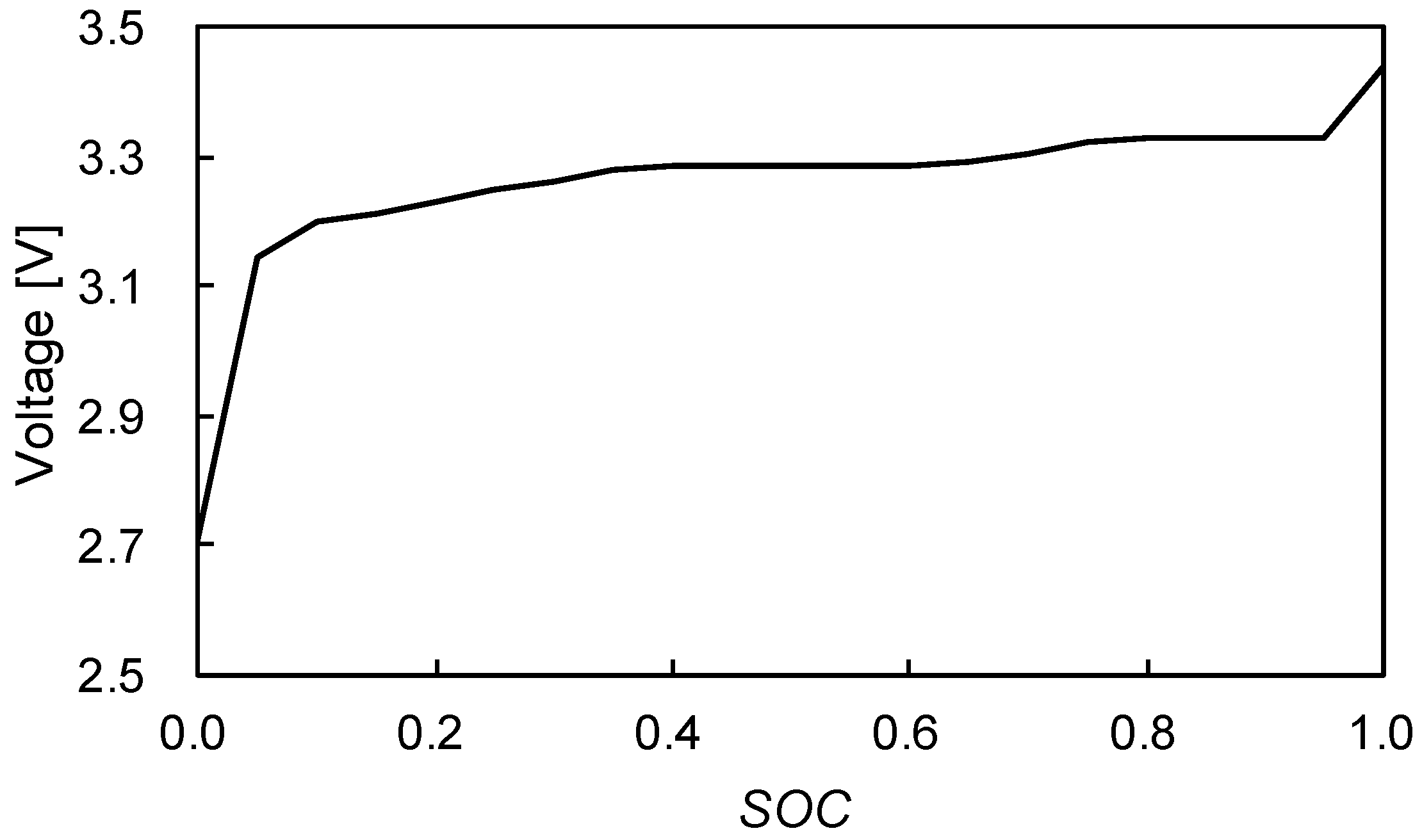
4.2. Battery Degradation based on Cycle Aging Model

Because of the battery’s characteristics of electrochemical dynamics and multi-physics coupling, it is difficult to monitor internal states accurately and robustly [22]. Although there is a conflict between energy consumption and battery life extension, there have been studies investigating methods to minimize both energy consumption and battery aging in terms of energy management [44]. Therefore, it is necessary to set a control strategy to optimize power management and battery aging without performance loss.

To estimate the impact of battery degradation occurred by charging from PV generation, cycle aging model is adopted as follows [30,48]:

$$Q_{cycle}=(\alpha SOC+\beta )\cdot (\frac{-E_a+\eta \cdot C_{rate}}{R_{gas}\cdot T_K})A{h}^z$$

(7)

where α and β are fitting coefficients, E_a is the activation energy, η is the compensation factor of C_rate, R_gas is the gas constant and T_K is the ambient temperature in [K]. Ah is the ampere-hour throughput and z is the power-law factor. The parameters such as fitting coefficients, activation energy, compensation factor, gas constant and power law factor used in the model are derived from [30,48]. Fitting coefficients α and β are defined by the SOC dependency and each fitting coefficient is varied by the SOC, 0.45, which is a critical point to define the low and high SOC.

And then, to investigate charging cycles of ESS during test periods, a discrete-time model of cycle aging can be defined as follows:

$$Q_{cycle,n+1}-Q_{cycle,n}=\Delta Ah\cdot z(\alpha SOC+\beta )\cdot (\frac{-E_a+\eta \cdot C_{rate}}{R_{gas}\cdot T_K})A{h}_n{}^{z-1}$$

(8)

where Q_cycle,n and Q_cycle,n+1 are the capacity loss at the time instants t_n and t_n+1, respectively; ΔAh is the ampere-hour throughput from t_n to t_n+1; Ah_n and Ah_n+1 are the accumulated ampere-hour throughput until the time instants t_n and t_n+1, respectively.

In this study, ampere-hour throughput is defined as the value that energy (E) is divided by nominal voltage (V_nominal) as follows:

$$\Delta Ah=\frac{1}{3600}{\displaystyle {\int }_{t_n}^{t_{n+1}}|C_{bat}(t)|dt}\approx \frac{E}{V_{\mathrm{nominal}}}$$

(9)

$$A{h}_{n+1}=A{h}_n+\Delta Ah$$

(10)

where C_bat is the battery current for charge, E and V_nominal are energy and a nominal voltage of the battery, respectively.

5. Results and Discussions

5.1. Results of PV Generation Forecasting

To calculate the statistical model parameters, two weeks of PV generation data and relevant datasets are used for training, and the selected model is tested with another ten days of data. When the performance of the selected models by varying the time lag (p) is tested, the multivariate model, MV_hour using 10 prior historical data with meteorological variables such as temperature, humidity, and irradiance, is determined as the best model, which has the least MAPE during the overall forecasting periods [45].

Figure 1 shows the PV forecasting using the selected short-term forecasting model. In both sunny and cloudy day, it shows excellent performance. As a result, MAPE result on a sunny day (day 4) is 0.227 and on a cloudy day (day 3) is 0.386.

The statistical test between forecasted and actual produced power is summarized in

Table 3. Comparison of mean absolute percentage forecast error (MAPE) between sunny days and cloudy days.

Weather Type	MVhour
Sunny	0.167
Cloudy	0.327

which presents the comparison of MAPE values between sunny days and cloudy days. For validating the performance of PV generation forecasting, the least value of MAPE is observed by the model differently. Table 3 shows that the performance of the model is better on sunny days (days 2, 4, 5, 8, 9 and 10).

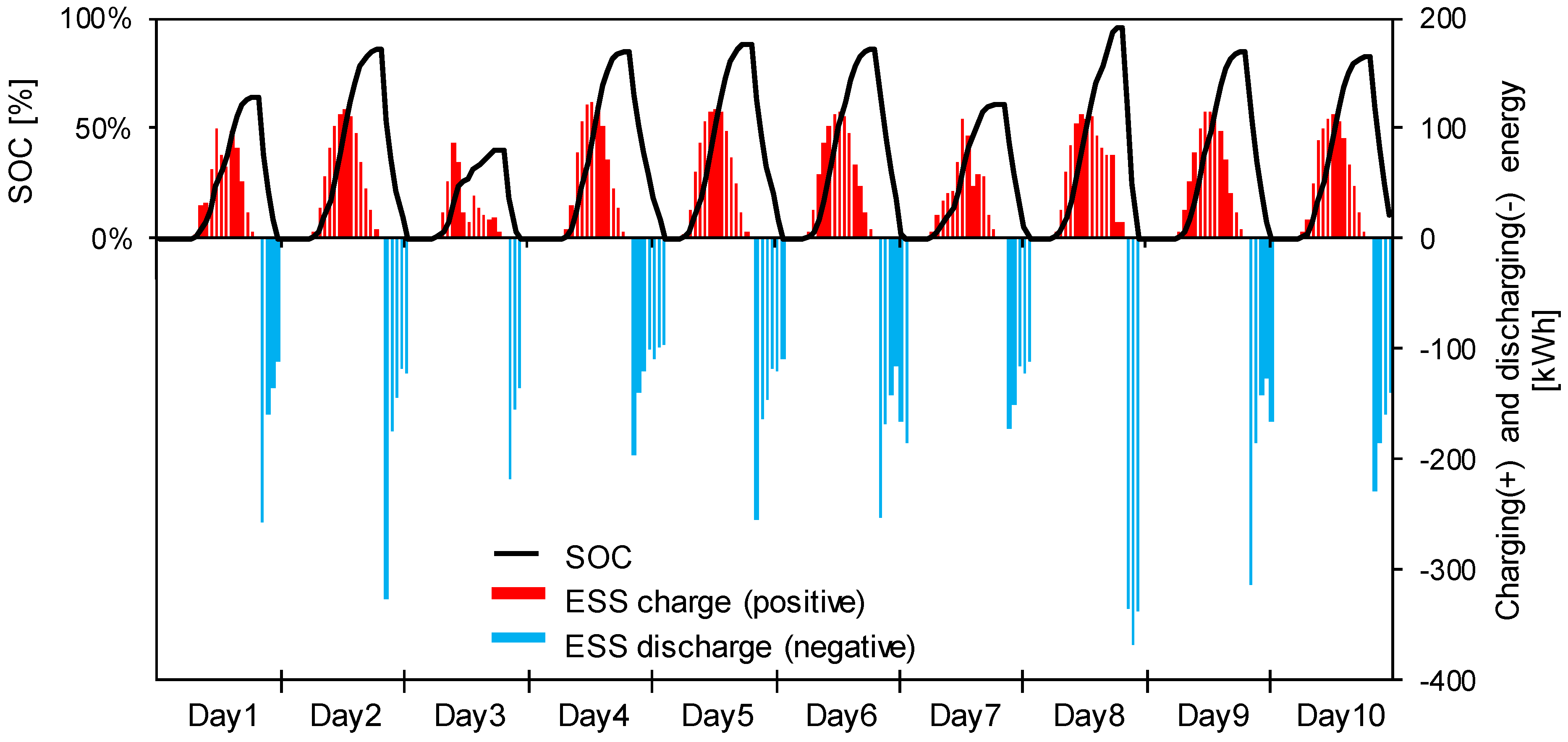
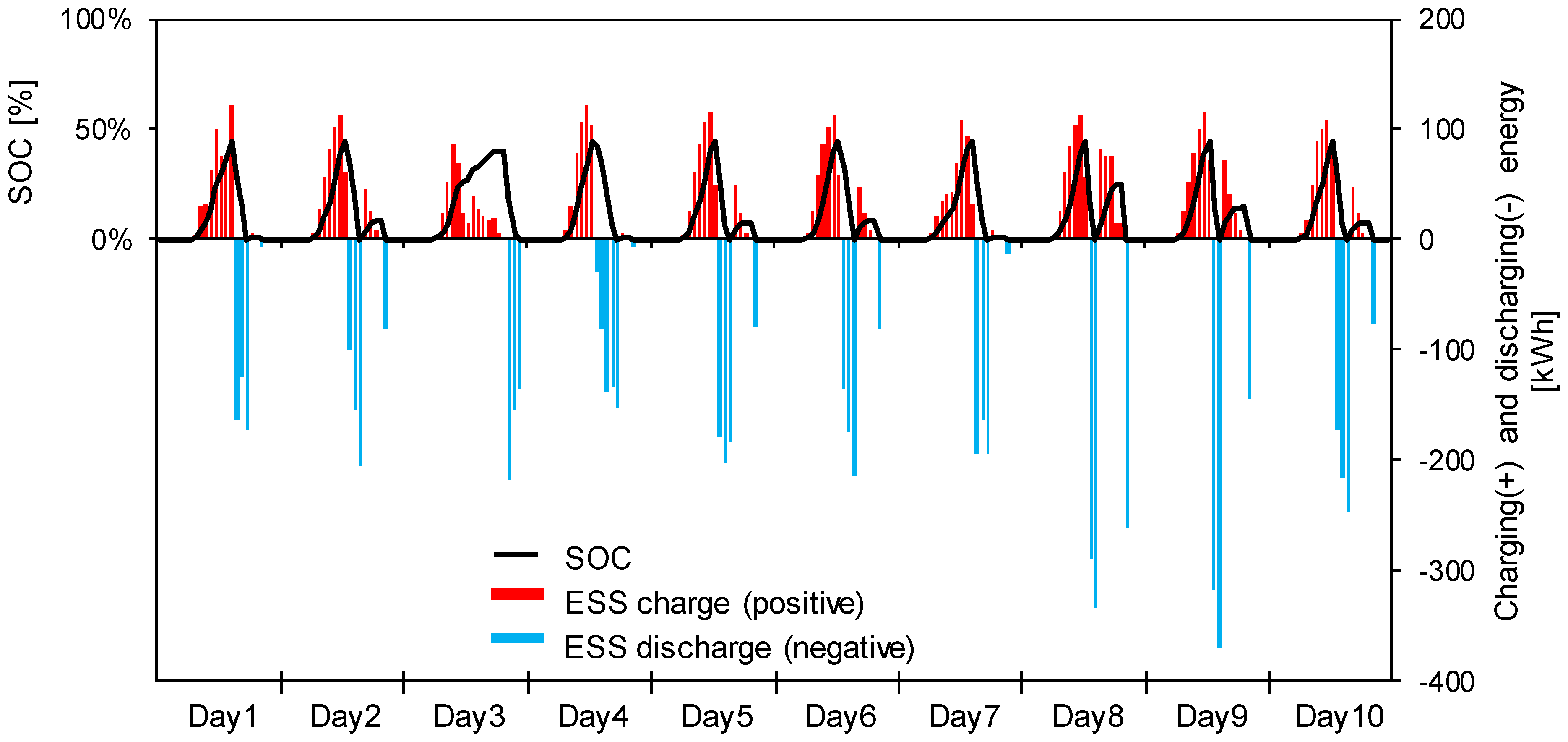
5.2. Simulation Results of ESS Charge and Discharge Operation Modes

According to self-consumption operation, the ESS is scheduled to charge and discharge energy to maximize charging PV generation based on PV forecasting. During testing periods of ten days, a day-ahead PV forecasting is performed by MV_hour model. While PV is generating electricity in the daytime and discharging the same amount to the load, the ESS starts charging.

In this study, we proposed two different ESS operation modes to investigate the difference in battery degradation depending on a different DOD (depth of discharge). In mode 1, the ESS is supposed to charge maximum PV generation and start discharging energy to the load for self-consumption when PV generation ends. In mode 2, the ESS is supposed to charge PV generation up to a certain point of the SOC, 0.45 which is the optimal value for investigating the operational stress factor of DOD.

Based on mode 1, Figure 2 shows the ESS is scheduled to charge the maximum amount of PV generation and discharge the same amount to the load. The daily peak of the SOC which is dependent on PV generation and the peak in cloudy days (days 1, 3 and 7) is relatively lower than sunny days.

Based on mode 2, the ESS is scheduled to charge the designated amount of PV generation and discharge the same amount to the load as shown in Figure 3. When the ESS reaches the SOC, 0%, the ESS operates to charge again until PV generation ends. The daily peak of the SOC is the same during testing periods and the ESS operates two cycles per day except day 3 when is not charged to the SOC, 0.45.

However, it is difficult to calculate the actual value of energy to be delivered to the load because the battery loses its capacity along with the charge and discharge cycles. Thus, using the battery cycle aging model is used to estimate capacity loss considering partial cycles at the different SOC ranges in a daily basis.

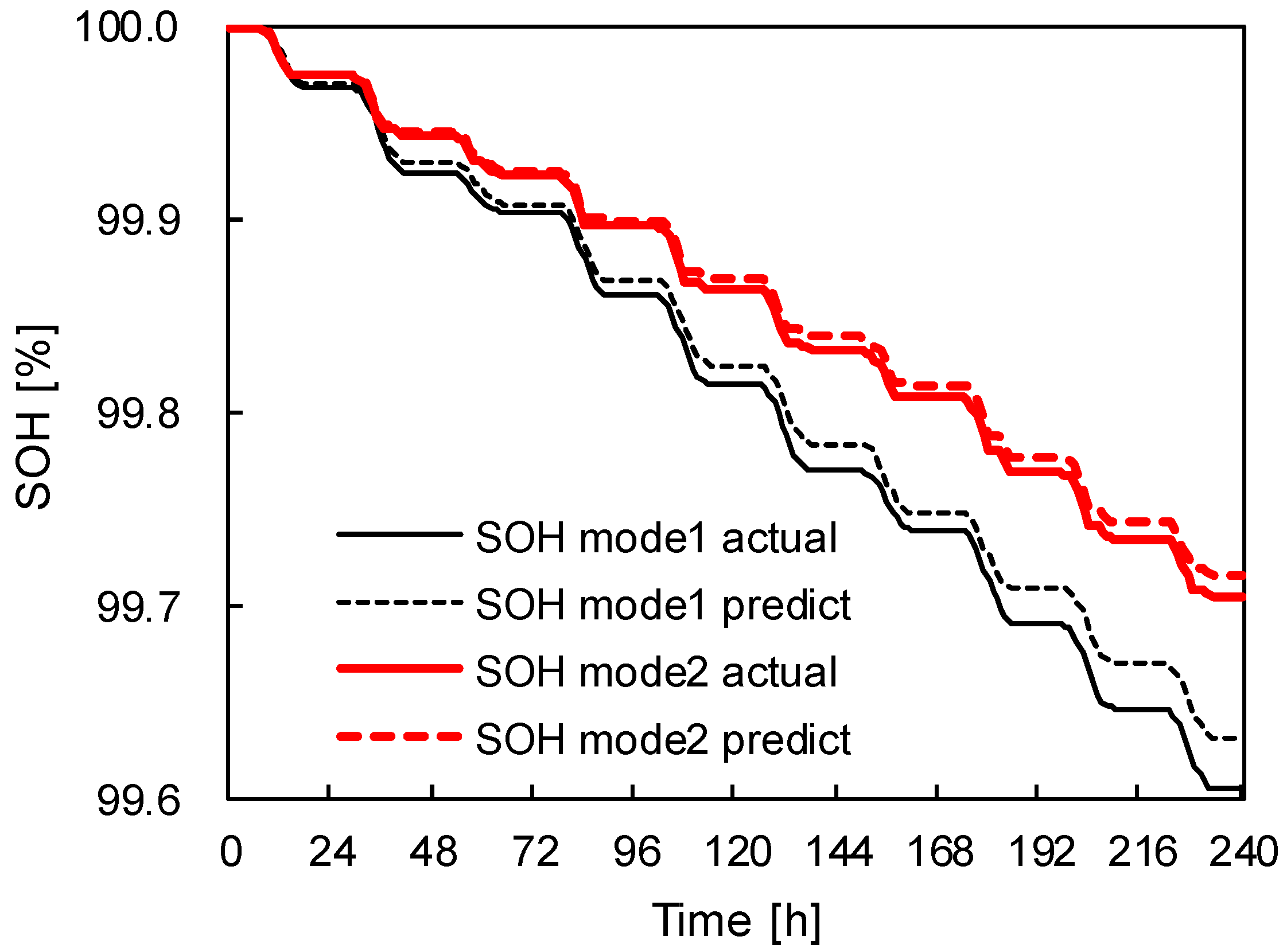
5.3. Results and Discussions

Starting with the ESS scheduling operation based on PV generation forecasting, capacity loss estimation using its hourly SOC data from the charging cycle is performed to evaluate the battery’s SOH. During whole testing periods, the results of battery degradation based on the ESS operation modes are compared to the result from the actual value of PV generation as shown in Figure 4. The battery degradation from the predicted ESS cycle in mode 1 is 0.37% and the SOH is 99.6% and the battery degradation in mode 2 is 0.29% and the SOH is 99.7%. In mode 2, the result of the SOH is 0.1% higher than mode 1 which indicates that the ESS operation with low DOD results in the less battery degradation than the result with high DOD. As can be seen, the difference of the SOH between battery degradation based on the actual value of PV generation and the predicted value is approximately 0.02% which is owing to the high accuracy of the PV forecasting model.

In general, the aging of the LFP battery indicates that the main factor of the battery degradation is the high SOC occurred by the charging process, which is due to the electrochemical charge overpotential when the SEI layer becomes large in high SOC region [49]. In the battery degradation model, the SOC coefficients (α and β) are reflected as shown in (7), which is changed at the SOC, 0.45. These coefficients are defined as the SOC dependence, which is determined from the curve fitting of experimental data [30]. The reason of the change can be identified through the SOC-open circuit voltage (OCV) relationship of the LFP battery as shown in Figure 5. The OCV is sharply changed in the low and high SOC region (0.9 and 0.05) and the other region is relatively flat because the SEI formation is varied little [49].

However, from only the SOC-OCV curve, the optimal threshold is hard to be determined for reflecting the SOC dependency. When the SOC-OCV relation is transformed to slope value as shown in Figure 6, the minimum value is at the SOC, 0.45. From this result, the coefficients (α and β) can be separately applied based on the SOC region and the optimal operation region of the battery is regulated under the SOC, 0.45 for the prolonged battery life.

6. Conclusions

This study presents PV generation forecasting models to find a control strategy for the integrated system of PV and ESS. Compared to the model research using the statistical model with a single variable, the PV forecasting technique with multivariate to increase the strength in a cloudy day can bring about the best prediction of PV generation. Those models are developed and trained with two weeks of 15-minutes interval generation data, weather data and solar radiation and tested with the next ten days of actual PV generation.

Derived from the comparison of the forecasting results, renewable energy forecasting can be separated by several steps. As mentioned earlier, the value of solar radiation should be input exogenously because the KMA weather forecast does not provide solar radiation. Since the Clear-Sky model is based on radiation estimation in a clear weather condition, other types of sky conditions should be modeled by different variables. Hence, depending on the sky condition, the MV_hour model operates with weather parameters. The result shows the proposed model has high performance both in sunny and cloudy days. However, it is necessary to consider predicting PV generation with an intelligent computational model that can perform better in the weather with high temporal variability PV generation to increase its confidence in forecasting.

Although EOL (End of life) is one of the most important factors for determining the battery replacement period, estimating EOL is difficult without measured data of battery capacity. In a realistic environmental condition, only voltage, current and energy can be acquired, and the capacity can be obtained limitedly by the specific experiment. In this study, a battery degradation model based on the data-driven method is utilized. From the experiment with the battery degradation model using parameters derived from experiments, it shows that the battery is degraded along with charging cycles during testing periods and variations in state of health are observed owing to the different characteristics of the battery according to the ESS operation modes. To separate the ESS operation modes, the optimal value of the SOC is set to investigate the impact of different DOD to battery degradation. From the simulation result, the result of the SOH in mode 2 which operates up to 0.45 of the SOC is 0.1% higher than mode 1 using full operation range. This result indicates that the ESS operation with low DOD results in less battery degradation than the result with high DOD. Finally, the simulation result leads to the conclusion that the battery degradation in different operation modes should be taken into account to extend the end of life efficiently.

However, avoiding high DOD to extend the EOL of the battery can bring a negative impact on the customer’s benefit. Therefore, future works will develop the capacity loss model with a wide range of battery aging data from experiments and suggest the optimal operating strategy under the various ESS operation mode. This preliminary research will provide effective guidelines for future research, to encourage more ESS integrating with renewable energy resources considering battery degradation.

References

1. UNFCCC. Adoption of the Paris Agreement. 2015. Available online: https://unfccc.int/process-and-meetings/the-paris-agreement/what-is-the-paris-agreement (accessed on 2 April 2020).
2. Beaudin, M.; Zareipour, H.; Schellenberglabe, A.; Rosehart, W. Energy storage for mitigating the variability of renewable electricity sources: An updated review. Energy Sustain. Dev. 2010, 14, 302–314. [Google Scholar] [CrossRef]
3. Suazo-Martínez, C.; Pereira-Bonvallet, E.; Palma-Behnke, R. A Simulation Framework for Optimal Energy Storage Sizing. Energies 2014, 7, 3033–3055. [Google Scholar] [CrossRef]
4. Suberu, M.Y.; Mustafa, M.W.; Bashir, N. Energy storage systems for renewable energy power sector integration and mitigation of intermittency. Renew. Sustain. Energy Rev. 2014, 35, 499–514. [Google Scholar] [CrossRef]
5. Denholm, P.; Ela, E.; Kirby, B.; Milligan, M. Role of Energy Storage with Renewable Electricity Generation; NREL/TP-6A2-47187; National Renewable Energy Lab. (NREL): Golden, CO, USA, 2010.
6. Akhil, A.A.; Huff, G.; Currier, A.B.; Kaun, B.C.; Rastler, D.M.; Chen, S.B.; Cotter, A.L.; Bradshaw, D.T.; Gauntlett, W.D. DOE/EPRI Electricity Storage Handbook in Collaboration with NRECA; Sandia National Laboratories: Albuquerque, NM, USA, 2015.
7. Eyer, J.M.; Corey, G.P. Energy Storage for the Electricity Grid: Benefits and Market Potential Assessment Guide: A Study for the DOE Energy Storage Systems Program; SAND2010-0815; Sandia National Laboratories: Albuquerque, NM, USA, 2010.
8. Rastler, D.M.; Electric Power Research Institute. Electricity Energy Storage Technology Options: A White Paper Primer on Applications, Costs and Benefits; Electric Power Research Institute: Palo Alto, CA, USA, 2010. [Google Scholar]
9. Bhatnagar, D.; Currier, A.; Hernandez, J.; Ma, O.; Kirby, B. Market and Policy Barriers to Energy Storage Deployment; SAND-2013-7606; Sandia National Lab. (SNL-NM): Albuquerque, NM, USA, 2013.
10. Medina, P.; Bizuayehu, A.W.; Catalão, J.P.S.; Rodrigues, E.M.G.; Contreras, J. Electrical Energy Storage Systems: Technologies’ State-of-the-Art, Techno-economic Benefits and Applications Analysis. In Proceedings of the 2014 47th Hawaii International Conference on System Sciences, Waikoloa, HI, USA, 6–9 January 2014; pp. 2295–2304. [Google Scholar]
11. Akinyele, D.O.; Rayudu, R.K. Review of energy storage technologies for sustainable power networks. Sustain. Energy Technol. Assess. 2014, 8, 74–91. [Google Scholar] [CrossRef]
12. Ela, E.; Milligan, M.; Bloom, A.; Botterud, A.; Townsend, A.; Levin, T. Evolution of Wholesale Electricity Market Design with Increasing Levels of Renewable Generation; National Renewable Energy Lab. (NREL): Golden, CO, USA, 2014.
13. Alarcon-Rodriguez, A.; Ault, G.; Galloway, S. Multi-objective planning of distributed energy resources: A review of the state-of-the-art. Renew. Sustain. Energy Rev. 2010, 14, 1353–1366. [Google Scholar] [CrossRef]
14. Nespoli, A.; Ogliari, E.; Leva, S.; Massi Pavan, A.; Mellit, A.; Lughi, V.; Dolara, A. Day-Ahead Photovoltaic Forecasting: A Comparison of the Most Effective Techniques. Energies 2019, 12, 1621. [Google Scholar] [CrossRef] [Green Version]
15. Kang, B.O.; Lee, M.; Kim, Y.; Jung, J. Economic analysis of a customer-installed energy storage system for both self-saving operation and demand response program participation in South Korea. Renew. Sustain. Energy Rev. 2018, 94, 69–83. [Google Scholar] [CrossRef]
16. Lee, W.; Kang, B.O.; Jung, J. Development of energy storage system scheduling algorithm for simultaneous self-consumption and demand response program participation in South Korea. Energy 2018, 161, 963–973. [Google Scholar] [CrossRef]
17. Park, M.; Kim, J.; Won, D.; Kim, J. Development of a Two-Stage ESS-Scheduling Model for Cost Minimization Using Machine Learning-Based Load Prediction Techniques. Processes 2019, 7, 370. [Google Scholar] [CrossRef] [Green Version]
18. Xu, B.; Oudalov, A.; Ulbig, A.; Andersson, G.; Kirschen, D.S. Modeling of Lithium-Ion Battery Degradation for Cell Life Assessment. IEEE Trans. Smart Grid 2018, 9, 1131–1140. [Google Scholar] [CrossRef]
19. Azuatalam, D.; Paridari, K.; Ma, Y.; Förstl, M.; Chapman, A.C.; Verbič, G. Energy management of small-scale PV-battery systems: A systematic review considering practical implementation, computational requirements, quality of input data and battery degradation. Renew. Sustain. Energy Rev. 2019, 112, 555–570. [Google Scholar] [CrossRef] [Green Version]
20. Li, X.; Wang, Z.; Zhang, L.; Zou, C.; Dorrell, D.D. State-of-health estimation for Li-ion batteries by combing the incremental capacity analysis method with grey relational analysis. J. Power Sources 2019, 410, 106–114. [Google Scholar] [CrossRef]
21. Berecibar, M.; Gandiaga, I.; Villarreal, I.; Omar, N.; Van Mierlo, J.; Van den Bossche, P. Critical review of state of health estimation methods of Li-ion batteries for real applications. Renew. Sustain. Energy Rev. 2016, 56, 572–587. [Google Scholar] [CrossRef]
22. Hu, X.; Feng, F.; Liu, K.; Zhang, L.; Xie, J.; Liu, B. State estimation for advanced battery management: Key challenges and future trends. Renew. Sustain. Energy Rev. 2019, 114, 109334. [Google Scholar] [CrossRef]
23. Asif, A.A.; Singh, R. Further Cost Reduction of Battery Manufacturing. Batteries 2017, 3, 17. [Google Scholar] [CrossRef]
24. Bloomberg New Energy Finance. A Behind the Scenes Take on Lithium-ion Battery Prices. 2019. Available online: https://about.bnef.com/blog/behind-scenes-take-lithium-ion-battery-prices/ (accessed on 2 April 2020).
25. Sachs, J.; Sawodny, O. A Two-Stage Model Predictive Control Strategy for Economic Diesel-PV-Battery Island Microgrid Operation in Rural Areas. IEEE Trans. Sustain. Energy 2016, 7, 903–913. [Google Scholar] [CrossRef]
26. Lai, C.S.; McCulloch, M.D. Levelized cost of electricity for solar photovoltaic and electrical energy storage. Appl. Energy 2017, 190, 191–203. [Google Scholar] [CrossRef]
27. Sidorov, D.; Muftahov, I.; Tomin, N.; Karamov, D.; Panasetsky, D.; Dreglea, A.; Liu, F.; Foley, A. A dynamic analysis of energy storage with renewable and diesel generation using Volterra equations. IEEE Trans. Ind. Inform. 2019, 16, 3451–3459. [Google Scholar] [CrossRef] [Green Version]
28. Chang, W.-Y. The State of Charge Estimating Methods for Battery: A Review. ISRN Appl. Math. 2013, 2013, 953792. [Google Scholar] [CrossRef]
29. Kim, W.-Y.; Lee, P.-Y.; Kim, J.; Kim, K.-S. A Nonlinear-Model-Based Observer for a State-of-Charge Estimation of a Lithium-Ion Battery in Electric Vehicles. Energies 2019, 12, 3383. [Google Scholar] [CrossRef] [Green Version]
30. Zhang, S.; Hu, X.; Xie, S.; Song, Z.; Hu, L.; Hou, C. Adaptively coordinated optimization of battery aging and energy management in plug-in hybrid electric buses. Appl. Energy 2019, 256, 113891. [Google Scholar] [CrossRef]
31. Debnath, K.B.; Mourshed, M. Forecasting methods in energy planning models. Renew. Sustain. Energy Rev. 2018, 88, 297–325. [Google Scholar] [CrossRef] [Green Version]
32. Ferrero Bermejo, J.; Gómez Fernández, J.F.; Pino, R.; Crespo Márquez, A.; Guillén López, A.J. Review and Comparison of Intelligent Optimization Modelling Techniques for Energy Forecasting and Condition-Based Maintenance in PV Plants. Energies 2019, 12, 4163. [Google Scholar] [CrossRef] [Green Version]
33. Tascikaraoglu, A.; Uzunoglu, M. A review of combined approaches for prediction of short-term wind speed and power. Renew. Sustain. Energy Rev. 2014, 34, 243–254. [Google Scholar] [CrossRef]
34. Wan, C.; Zhao, J.; Song, Y.; Xu, Z.; Lin, J.; Hu, Z. Photovoltaic and solar power forecasting for smart grid energy management. CSEE J. Power Energy Syst. 2015, 1, 38–46. [Google Scholar] [CrossRef]
35. Botterud, A. Forecasting renewable energy for grid operations. In Renewable Energy Integration; Academic Press: Cambridge, MA, USA, 2017; pp. 133–143. [Google Scholar]
36. Notton, G.; Nivet, M.L.; Voyant, C.; Paoli, C.; Darras, C.; Motte, F.; Fouilloy, A. Intermittent and stochastic character of renewable energy sources: Consequences, cost of intermittence and benefit of forecasting. Renew. Sustain. Energy Rev. 2018, 87, 96–105. [Google Scholar] [CrossRef]
37. Rudin, C.; Waltz, D.; Anderson, R.N.; Boulanger, A.; Salleb-Aouissi, A.; Chow, M.; Dutta, H.; Gross, P.N.; Huang, B.; Jerome, S. Machine learning for the New York City power grid. IEEE Trans. Pattern Anal. Mach. Intell. 2012, 34, 328–334. [Google Scholar] [CrossRef] [Green Version]
38. Deo, R.C.; Wen, X.; Qi, F. A wavelet-coupled support vector machine model for forecasting global incident solar radiation using limited meteorological dataset. Appl. Energy 2016, 168, 568–593. [Google Scholar] [CrossRef]
39. Jianzhou, W.; Na, Z.; Lu, H. A novel system based on neural networks with linear combination framework for wind speed forecasting. Energy Convers. Manag. 2019, 181, 425–442. [Google Scholar]
40. Wang, H.Z.; Lei, Z.X.; Zhang, X. A review of deep learning for renewable energy forecasting. Energy Convers. Manag. 2019, 198, 111799. [Google Scholar] [CrossRef]
41. Korea Meteorological Administration Official Webpage. Available online: http://web.kma.go.kr/eng/biz/forecast_03.jsp (accessed on 2 April 2020).
42. Masters, G.M. Renewable and Efficient Electric Power Systems; John Wiley & Sons: Hoboken, NJ, USA, 2013. [Google Scholar]
43. Mousavi Maleki, S.A.; Hizam, H.; Gomes, C. Estimation of Hourly, Daily and Monthly Global Solar Radiation on Inclined Surfaces: Models Re-Visited. Energies 2017, 10, 134. [Google Scholar] [CrossRef] [Green Version]
44. Antonanzas, J.; Osorio, N.; Escobar, R.; Urraca, R.; Martinez-de-Pison, F.J.; Antonanzas-Torres, F. Review of photovoltaic power forecasting. Sol. Energy 2016, 136, 78–111. [Google Scholar] [CrossRef]
45. Lee, M.; Lee, W.; Jung, J. 24-Hour photovoltaic generation forecasting using combined very-short-term and short-term multivariate time series model. In Proceedings of the 2017 IEEE Power & Energy Society General Meeting, Chicago, IL, USA, 16–20 July 2017; pp. 1–5. [Google Scholar]
46. Sun, C.; Rajasekhara, S.; Goodenough, J.B.; Zhou, F. Monodisperse porous LiFePO4 microspheres for a high power Li-ion battery cathode. J. Am. Chem. Soc. 2011, 133, 2132–2135. [Google Scholar] [CrossRef] [PubMed]
47. Miao, Y.; Hynan, P.; von Jouanne, A.; Yokochi, A. Current Li-Ion Battery Technologies in Electric Vehicles and Opportunities for Advancements. Energies 2019, 12, 1074. [Google Scholar] [CrossRef] [Green Version]
48. Suri, G.; Onori, S. A control-oriented cycle-life model for hybrid electric vehicle lithium-ion batteries. Energy 2016, 96, 644–653. [Google Scholar] [CrossRef]
49. Weißhar, B.; Bessler, W.G. Model-based lifetime prediction of an LFP/graphite lithium-ion battery in a stationary photovoltaic battery system. J. Energy Storage 2017, 14, 179–191. [Google Scholar] [CrossRef]
Figure 1. MVhour model forecast; (a) PV forecasting on a sunny day; (b) PV forecasting on a cloudy day.
Electronics 09 00701 g001
Figure 2. Self-consumption ESS schedule in mode 1.
Electronics 09 00701 g002
Figure 3. Self-consumption ESS schedule in mode 2.
Electronics 09 00701 g003
Figure 4. Comparison of the day-ahead battery degradation estimations.
Electronics 09 00701 g004
Figure 5. Relationship between the state of charge (SOC)-open circuit voltage (OCV) curve.
Electronics 09 00701 g005
Figure 6. Slope of the linearized SOC-OCV curve.
Electronics 09 00701 g006