Towards Traffic Identification and Modeling for 5G Application Use-Cases

Abstract

To analyze next-generation mobile networks properly, there is a need to define key performance indicators (KPIs). Testing signaling only or just partial domains of the network have been replaced with end-to-end testing methodologies. With the appearing of machine-to-machine (M2M) applications, this question became even harder, since there is no direct user feedback. Quality of experience cannot be measured accurately in M2M applications, even if the network operates correctly and without failures. There are dozens of new—but theoretical—use-cases for 5G; however, these are not tested on a live network. The modeling methodology used throughout the paper follows the steps of observation, analysis, model creation, implementation, and verification. The first part of the paper examines the three application-types: enhanced mobile broadband (eMBB), critical Internet of Things (cIoT), and mass Internet of Things (mIoT). Afterwards, we introduce the main traffic characteristics based on current mobile networks’ traffic patterns and measurements. Considering the measurement results, we introduce a methodology and define traffic models for the simulation of different application-types. To validate these models, we compare the generated artificial traffic with real traffic patterns. In the second part of the paper, we examine what the main effects of these traffic patterns on a domestic 5G test-network are. Finally, we suggest some considerations on the possible main impacts regarding 5G network design.

1. Introduction

Their rapid spread and popularity prove the success of cellular networks all around the world; therefore, advanced mobile networks are major components of the digital future. Since the boundaries between mobile and broader (industrial) digital systems continue to blur in various senses, many telco operators are moving beyond their traditional telecommunication businesses to explore new opportunities [1].

Nevertheless, smartphones will still remain the focal point of the consumer internet economy in the upcoming years [2]—the volume of connected devices is higher than ever. Today’s digital consumers will likely to become tomorrow’s augmented customers, adopting emerging technologies such as virtual reality and Artificial Intelligence (AI). The telco sector is under pressure due to slowing unique subscriber growth and regulatory interventions. However, upcoming new opportunities have the potential to provide the uplift for mobile operator revenue. Mobile operators are pursuing new incremental revenue opportunities in content-, Internet of Things (IoT)-, and 5G-related use cases. They are looking for expanding their role in the value chain, from providing capabilities or tools. On one hand, they tend to move from merely supporting their partners to create IoT solutions and becoming end-to-end IoT solution providers themselves [3]. On the other hand, an increasing number of telco operators are entering the content space or strengthening their existing content offerings. They are creating content themselves or making partnerships with Over-The-Top (OTT) video service providers [4].

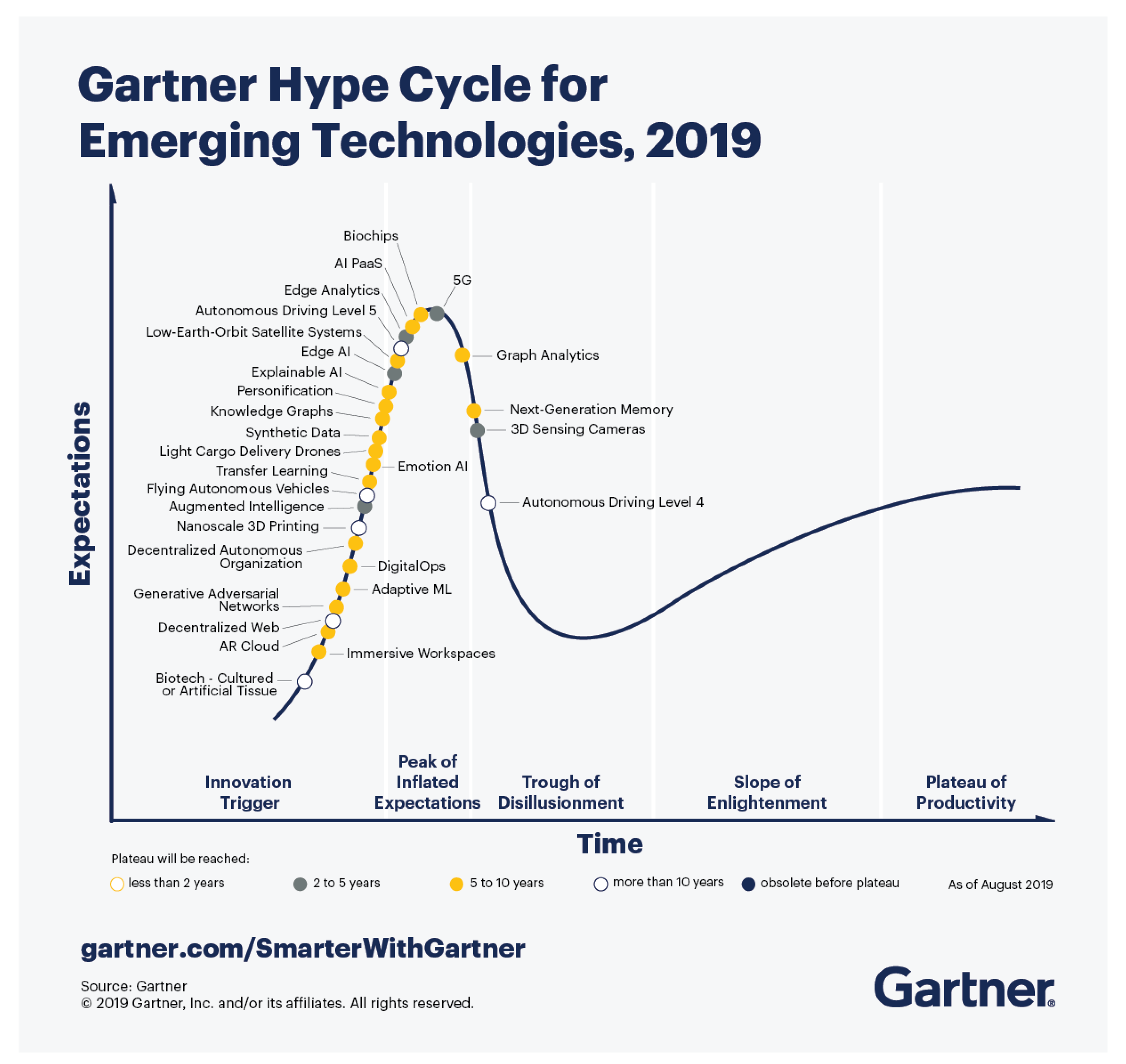
5G is now upon us, holding the promise of multiple exciting new services and applications. It arguably is one of the most hyped technology currently. According to the Gartner Hype Cycle report (Figure 1), the International Telecommunication Union and other standards bodies are expected to ratify full 5G technical standards by 2020. Another Gartner report claims that 5G wireless network infrastructure revenue will reach $4.2 billion in 2020, an 89% increase from 2019 revenue of $2.2 billion [5].

With the emerging new applications, accurate traffic identification and measurements are crucial elements of creating high-quality network business intelligence and network policy control. Content service providers (CSP) can not generate new subscriber services, optimize resource utilization, and ensure correct charging without measuring and monitoring the traffic flow on their current networks. There are several techniques to identify traffic patterns, gain additional information and measure quantities, ranging from relatively simple (e.g., statistics) to extremely complex (e.g., machine learning). It is not fully understood how the various user demands can affect the traffic flows since there are no KPIs defined yet to quantify these effects. Every element of the cellular network need to co-operate to serve user demands, deal with traffic peaks, and have to obey quality of service (QoS) guarantees. To do this, traffic-related characteristics should be determined and should be used during network planning, optimization, and service shaping. This is exactly what motivates our work.

Regarding 5G cellular traffic modeling and use-case traffic pattern analysis, so far, there are just a few published measurement results on lab, pilot, or live networks. In addition to the measurements over the 5G infrastructure, the description of the upcoming use-cases needs to be more accurate. Publications of next-generation protocols and even the general formalism of 5G are hard to find at this stage, hence posing a research gap.

It has not yet been examined how the new generation application traffic types or the currently existing ones will affect the live 5G network and how the user experience will change in the future. As part of the preparation for the upcoming changes, the main use-cases regarding data and signaling resource allocation demands are to be defined and well understood. While the related standard, 3rd Generation Partnership Project (3GPP) TS22.261 [7] set the scene for a lot of use-cases, this current paper extends the perspective with real-life network measurement results on the 4G live network. The results support the understanding of the current cellular network usage scenarios. Moreover, these results can help to define their traffic patterns and give a methodology to describe the traffic of applications—separately as well as aggregated—hence facilitating traffic modeling.

The contributions of this paper are the following:

• analysis of live 4G user as well as control traffic to identify usage patterns and to facilitate modeling;
• analysis of live 4G control traffic to provide input for modeling;
• applying the approach of “observation–analysis–model creation–traffic generation–verification” for 5G traffic modeling based on 4G traffic observations;
• active verification of a 5G testbed based on the model-based, generated traffic;
• sharing the QoS measurement results (throughput, latency, jitter) of the 5G testbed—for eMBB, mIoT, but not for critical IoT traffic.

The paper is structured as follows: Section 2 briefly presents the state of art and trends of the telecommunication industry. First, the key features of 4G application traffic types and their features are introduced. Afterwards, the main principles and expectations for 5G are presented. Section 3 introduces the main 5G use-cases, presents the architectural elements of the 5G non-standalone network, and gives you an overview of the limitations and capacity considerations for each network element. Section 4 presents the modeling approach we followed, which consists of the steps “observation–analysis–model creation–traffic generation–verification”. Section 5 explores the user traffic modeling methodology and describes what parameters can be used to find the predecessors of 5G use-cases on existing 4G networks. As part of this, we extract the characteristics of four, partly different usage scenarios and build a traffic model for these to be used during 5G performance and quality of service analysis. Section 6 describes the 5G measurement environment, then the design, implementation, execution, and analysis of measurements based on the earlier-described use-cases. Section 7 summarizes the measurement results, whereas Section 8 draws conclusions, and highlights the main findings of our work.

2. Related Works

Both the growing number of users and their individual expectations drive the need for better QoS and new services. 4G became the leading cellular technology across the world in the previous years, overtaking 2G with 3.4 billion connections, accounting worldwide [8]. The growth of 4G growth will continue, replacing 3G and 2G infrastructures in the following years – meanwhile, 5G is becoming reality. Current 5G research trends are summarized in [9]:

• the architecture itself,
• scalability, massive deployments,
• interoperability and dense HetNets,
• security and privacy concerns,
• issues related to slicing, software defined networks (SDN) and network function virtualization (NFV) issues,
• device-to-device communication,
• energy efficiency,
• mobile edge computing and the edge-cloud,
• artificial intelligence and
• private campus networks and production-related applications, just to mention a few.

The following subsections first summarize the actual cellular network trends, then provide an overview of 5G features, and finally list some of the related traffic modeling articles.

2.1. Cellular Network Trends

Each generation of mobile technology has been motivated by the need to meet a requirement identified between that technology and its predecessor. The transition from 2G to 3G was expected to enable mobile internet on consumer devices, but while it did, added data connectivity issues. In 3G a giant leap in terms of consumer experience occurred, as the combination of mobile broadband networks and smartphones brought about a significantly enhanced mobile internet experience. It eventually led to the application-centric world as we see today. From social media through music and video streaming to controlling your home appliances from anywhere in the world, mobile broadband has brought enormous benefits. It has fundamentally changed the lives of many people through services provided both by operators and third-party players.

The transition from 3G to 4G services has offered users access to considerably faster data speeds and lower latency [10]. The way that people access and use the internet on mobile devices continues to change dramatically. Operators often cite an increased level of video streaming by customers on 4G networks as a major contributing factor to this. The IoT has also been discussed as a key aspect for 4G, but in reality, the challenge of providing low power, long-ranging networks to meet the demand for widespread M2M deployment is not specific to 4G or, indeed, 5G.

According to Cisco’s global mobile data traffic forecast [11] on the global market of telecommunication, the relative share of 4G-capable devices and connections surpassed all other connection types in 2019 (Figure 2). There were 42% 4G connections in 2018, but by the end of the forecast period, there will be 46% 4G connections, while 3G and below will only have 29% of connections. By 2023, there will be 11% of all devices and connections with 5G capability. The network evolution toward more advanced networks is happening both across the end-user device segment and within the M2M connections category.

There are many ideas that exist on the purpose of 5G will become as an infrastructure. One of them is that mobile operators would create a blend of pre-existing technologies covering previous generation technologies, WiFi, low power wide area (LPWA) and others to allow higher coverage and availability, and higher network density in terms of cells and devices. Another commonly reflected idea is that 5G will be an enabler to more excellent connectivity for M2M services and the IoT. This vision may include a new radio technology to enable low power, low throughput field devices with long life-cycles of ten years or more. Another one is more of the traditional ‘generation-defining’ view. It has specific targets for data rates and latency being identified, such that new radio interfaces and core architecture can be assessed against such criteria. This makes a clear demarcation between a technology that meets the criteria for 5G, and which does not.

LPWA connectivity is explicitly meant for M2M modules that require low bandwidth and extensive geographic coverage [12]. It provides high coverage with low power consumption, module, and connectivity costs, thereby creating new M2M use cases for mobile network operators (MNOs) that cellular networks alone could not have addressed. Examples include utility meters in residential basements, gas or water meters that do not have power connection, street lights, and pet or personal asset trackers. As the forecast states, the share of LPWA connections (all M2M) will grow from about 2 percent in 2017 to 14 percent by 2022, from 130 million in 2017 to 1.8 billion by 2022.

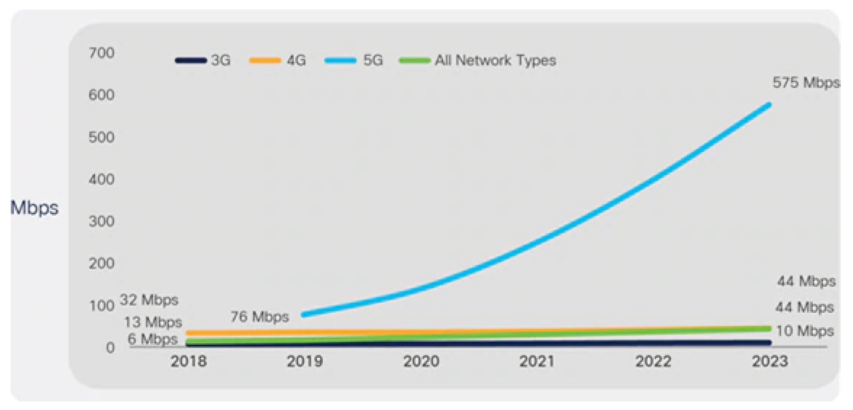
Regarding traffic, Cisco’s forecast [11] mentions, the average mobile network connection speed in 2018 was 13.2 Mbps. In the future, it will continue to grow, the average speed will more than triple and will be 43.9 Mbps by 2023 (Figure 3). The incrementing proportion of 4G mobile connections and the ascension of 5G connections are crucial factors promoting the incrementation in mobile speeds over the forecast period. The effect of 4G and 5G connections on traffic is significant, as they contribute to a disproportionate magnitude of mobile data traffic.

It is anticipated that 5G deployment will probably not be as quick as 4G’s was. Slow expansion of 5G means that being first to market with 5G is less important than having a long-term strategy for 5G investment that creates value for customers. The rollout of 4G holds some important lessons. Since the quality of the mobile broadband experience relies heavily on network capability and capacity, network tests and consumer mobile broadband satisfaction tests will be even more important in the 5G world than for 4G or 3G. For the same reasons, it is also anticipated by the operators that 5G devices will take time to roll out and become affordable.

2.2. The Main Features of 5G

Primary improvements of 5G over 4G include high bandwidth, broader coverage, and ultra-low latency [13]. These features combined with enhanced power efficiency, cost optimization, high-precision positioning, massive IoT connection density and dynamic allocation of resources based on awareness of content, user, and location make 5G a flexible as well as a transformative technology. 5G will be able to accommodate IoT applications such as environment monitoring, various sensors, and meters at the low end of the IoT spectrum. It also aims to support autonomous cars, smart grid, factory automation, and other tactile Internet-driven applications such as augmented and virtual reality.

The expectations are quite diverse, although the actual value of 5G will lie beyond providing connectivity itself, and even beyond advanced application and massive IoT enablement. 5G can genuinely unlock the business value for the customers and create new revenue opportunities for the providers with enhanced network edge capabilities, data analytics, machine learning and artificial intelligence services. This technology is expected to solve or at least significantly improve frequency licensing and spectrum management issues. Currently, there are various standards, bodies, regulatory agencies, and industry consortium focused on concerted efforts to resolve 5G issues, such as network standardization, spectrum availability and return of investment strategies to justify the investment associated with new infrastructure transitions and deployments. Given these evolving technology and business dynamics, we anticipate that some large scale commercial 5G deployments may not be executed until after the current forecast period (after 2022). A large number of mobile carriers perceive 5G as imperative for future growth and long-term sustainability.

As a result of this blend of requirements, many of the industry initiatives that have progressed with work on 5G identify a set of eight requirements [14]:

• 1–10 Gbps connections to endpoints in the field (i.e., not theoretical maximum);
• 1 millisecond end-to-end delay (latency);
• 1000× bandwidth per unit area;
• 10–100× number of connected devices;
• (Perception of) 99.999% availability;
• (Perception of) 100% coverage;
• 90% reduction in network energy usage;
• Up to ten-year battery life for low power, machine-type devices.

These requirements are specified from different perspectives, and they do not make an entirely coherent list. It is difficult to conceive of a new technology that could meet all of these conditions simultaneously, and 5G will not be capable of satisfying all of these requirements at the same time.

Equally, while these eight requirements are often presented as a single list, no use case, service or application has been identified that requires all eight performance attributes across an entire network simultaneously. Indeed some of the requirements are not linked to use cases or services but are instead theoretical goals of how networks should be built, independent of service or technology—no use case needs a network to be significantly cheaper, but every operator would like to pay less to build and run their network. It is more likely that various combinations of a subset of the overall list of requirements will be supported "when and where it matters." ITU-R has defined the following main usage scenarios for IMT for 2020 and beyond in their Recommendation ITU-R M.2083 [15]:

• eMBB to deal with hugely increased data rates, high user density and very high traffic capacity for hotspot scenarios as well as seamless coverage and high mobility scenarios with still improved used data rates;
• Massive Machine-type Communications (mMTC) also known as mIoT for the IoT use-cases, requiring low power consumption and low data rates for vast numbers of connected devices;
• Ultra-reliable and Low Latency Communications (uRLLC) or cIoT to cater for safety-critical and mission-critical applications.

2.3. Traffic Modeling—A Brief Overview

The composite model described in this paper incorporates building blocks from earlier published modeling methods, briefly summarized in the following references.

Chandrasekaran [16] gives an overview of the various traffic models. The Cisco paper [17] on voice over internet protocol (VoIP) traffic patterns compares various traffic models for voice calls, including Erlang B and C, Extended Erlang B, Engset, Poisson, EART/EARC, Neal-Wilkerson, Crommelin, Binomial, and Delay.

The UMTS Forum Report 44 [18] is built on a traffic model which distinguishes service categories (video/audio streaming, mobile gaming, etc.), device categories (smartphones, tablets, connected embedded devices, etc.) and various subscriber activity patterns. These components contribute to the overall traffic models through parameters such as traffic per service/device, device mix, upload/download direction, the period of the day/week/year, and others.

Aalto et al. [19] compared various scheduling algorithms from link delay and fairness aspects, and found that scheduling algorithms in the access network have their impact on the observed traffic in the core network.

Traffic modeling has a huge literature, and the modeling based on arrival processes, on-off behavior, long-range dependent behavior, and heavy-tailed file size distributions are researched deeply. To get the traffic generator’s composite model realistic, these traffic-features should also be considered—both during the modeling and the verification phases.

Arlitt et al. published a comprehensive workload characterization study of Internet Web servers in 1997 [20], which they repeated ten years later [21]. Although traffic volume increased 30-fold over the elapsed years, they found that some key workload characteristics seem to persist over time. These include one-time referencing behaviors, high concentration of references, heavy-tailed file size distributions, non-Poisson aggregate request streams, Poisson per-document request streams, and the dominance of remote requests. They speculate that these invariants will continue to hold in the future, because they represent fundamental characteristics of how information is organized, stored and accessed on the Web.

Park and his colleagues [22] found that self-similarity in network traffic can arise due to the reliable transfer of files drawn from heavy-tailed distributions. Crovella et al. [23] concluded that the heavy-tailed nature of transmission and idle times is not primarily a result of protocols or user preference, but rather some basic properties of information storage and processing: both file sizes and user “think times" are strongly heavy-tailed. Shaikh et al. [24], examining the on-off model, propose a wavelet-based criterion to differentiate between the network-induced traffic gaps and user think times.

Bregni and Jmoda [25] exhaustively analyze long-range dependency and provide an accurate estimation for the Hurst parameter. They attribute this to the moderating effect of TCP on network performance in the presence of highly bursty traffic. According to their observations, performance declines drastically with increasing self-similarity when a UDP-like unreliable transport mechanism was employed. Sahinoglu et al. [26] report that their research aims are to detect self-similarity in real-time, and come up with a measure of self-similarity such that this measure can be input for the optimization of resource allocation algorithms. Wilson [27] overview concludes that non-self-similar models (such as the Poisson or Markov Modulated Poisson Process or packet trains) are not adequate for modeling the self-similar properties of network traffic at larger time scales. This gave rise to self-similar models such as the Pareto and Weibull distribution processes. Vishwanath et al. [28] set off for implementing the Swing network emulation environment, which automatically extracts distributions for user, application and network behavior, and is capable of reproducing traffic burstiness (thus demonstrating self-similar properties) across a range of timescales.

Andreev et al. [29] propose a practical traffic generation model based on the discrete-time batch Markovian process with the intent to fill the gap between the analytically complex models discussed in academic publications and the simpler, more practical models preferred by standardization bodies.

Terdik and Gyires [30] believe that it is time to reexamine the Poisson traffic assumption because the amount of Internet traffic grows dramatically, and any irregularity of the network traffic, such as burstiness, might cancel out because of the enormous number of different multiplexed flows.

As this section has shown, traffic modeling has wide and often diverging aspects. Beside following the general idea of modeling systems, we have incorporated the packet- and flow-based traffic-separation ideas and used the statistical distribution features and complex metrics of various traffic patterns. Although our composite model allows utilizing features related to arrival processes and self-similarity, we have not implemented those in the currently presented models.

3. Service Provider Perspective on 5G Traffic and the Network

Standardization bodies continuously keep an eye on the new opportunities, enabler functions and technologies that can define the upcoming use-cases. The user expectations keep growing every year – as well as the performance of cellular devices. 5G delivers basic connectivity as well as mobile data services that are always available to customers when they need them. 5G will enable networking services for applications with high computing requirements. The growing sophistication of Artificial Intelligence and the availability of cheap computing power will drive the widespread adoption of digital assistants, intelligent IoT nodes, and automated industrial processes.

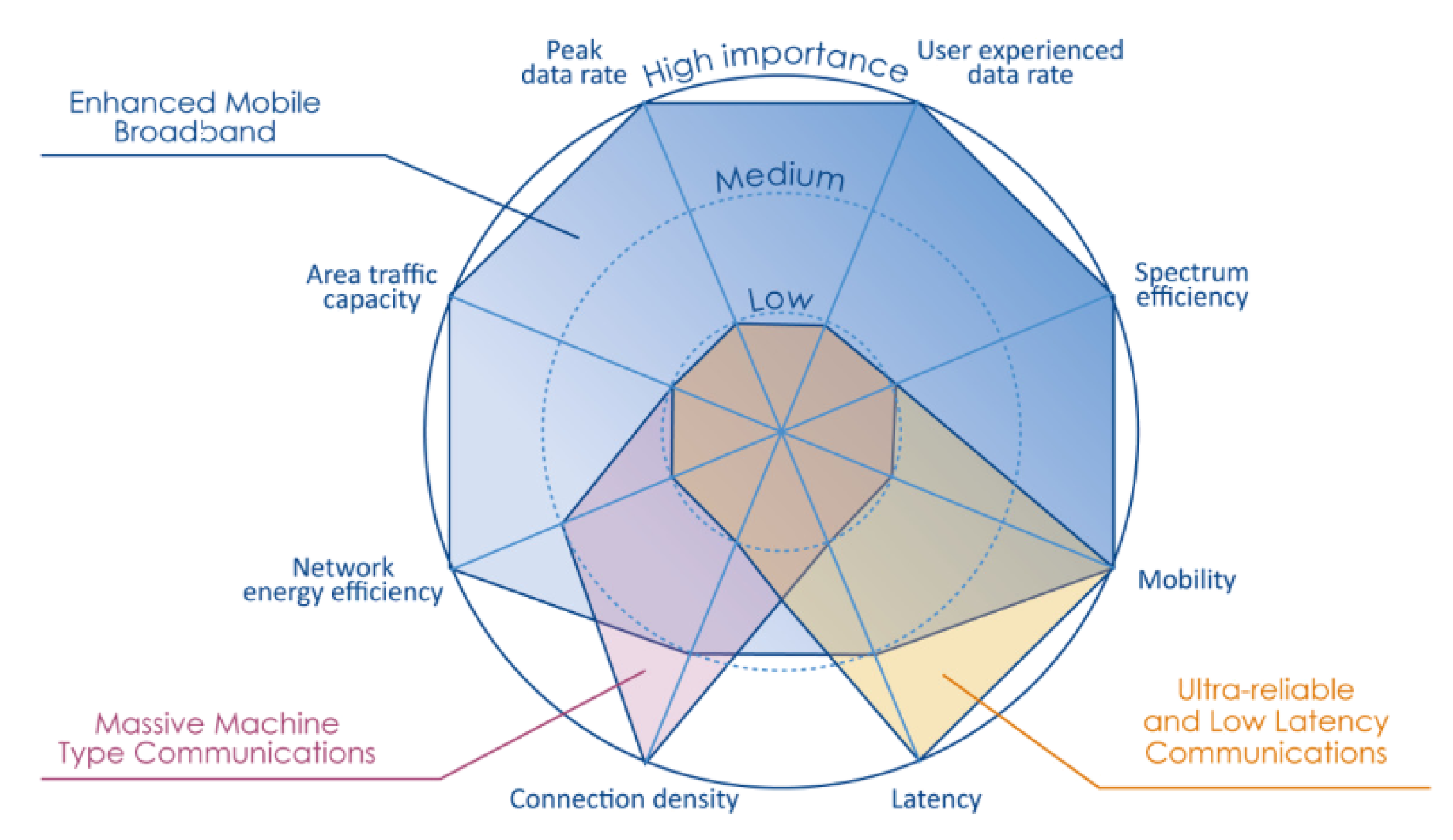
Industry stakeholders and standardization bodies have identified several potential use cases for 5G, which pose demands for very diverse requirements. Most of these can be identified within three primary categories [31]: enhanced Mobile Broadband, massive IoT, and critical IoT (

Table 1. Use-cases and their corresponding, important parameters (Scale-importance: tolerant/low: 1, normal/medium: 3, major/high: 5).

Use-Case	eMBB	mIoT	cIoT
High bandwidth	5	1	1
Low latency	4	1	5
High reliability	4	1	5
Low jitter	3	1	5
Cell handover	5	1	4
Transmit power control	5	1	5
High security	4	1	5
High availability	3	3	4
High number of devices	2	5	2
LAN-WAN connection	5	1	1

and Figure 4).

3.1. Enhanced Mobile Broadband

eMBB will be the key proposition in early 5G deployments and will drive increased performance, functionality and efficiency. Out of these three use-cases, “Massive Broadband” is currently the most widely spread – subscribers are humans. The main requirement is to serve the user with as high data rate as possible, while keeping the latency and end-to-end response time low. It will support high definition video (TV and gaming), and smart city services (video cameras for surveillance). eMBB is targeting mainly general subscribers; their primary interest is to provide better QoS and user experience. Furthermore, it provides higher bandwidth and higher speeds for densely populated urban areas and event locations, such as stadiums. Broadband connectivity is expected from application services delivering augment and virtual reality, 4K/8K video streaming, and seamless cloud services on demand.

The push for eMBB in 5G is a continuation of the 4G mobile broadband transformation. The emphasis on eMBB will sustain the 5G business case, and drive 5G network investment, in the absence of any new mobile use cases. However, under current operator business models, building a ubiquitous 5G network to support the latency that autonomous vehicles require remains as unrealistic as funding the level of small cell deployment needed to support a seamless augmented reality experience.

3.2. Ultra Reliable Low Latency Communications

The user base of cIoT on the current cellular networks is negligible. This is due to the fact that service providers can not guarantee sub 20 ms latency and a high level of QoS in case of packet delivery. However, the main goals of uRLLC include very low latency, packet delivery guarantees, and accurate user localization. Service Providers (SP)s offer various opportunities for the possible use-cases, but concrete business needs do not exist yet. From a technical point of view, examining cIoT is maybe the most labor-intensive task among the three main 5G use-cases, as concrete user demands are not known. These use cases serve the real-time interactions for mission-critical communications, such as autonomous driving, robotic control for industrial automation, drones and remote surgery medical care systems. The tactile response time is expected to be less than 1 ms. Public safety and emergency services supporting disaster response and location services are critical for lifeline communication and recovery [32].

3.3. Massive IoT

The need for machine-to-machine and machine-to-human communication is growing rapidly. Therefore, massive IoT will be a key application type in 5G. In mIoT, 5G network has to be capable of dealing with the high density of IoT devices. It will serve billions of low-cost, long-range, ultra-energy efficient devices, machines and things that need connectivity from remote locations as well as cloud applications with periodic, infrequent communication. It is important that devices have to be able to connect as groups to the network without individual authentication. mIoT devices need to be cheap but unlike eMBB devices, they nor have high calculation capacity processors neither memory capacity. Also, their radio receiver/transceiver module has to be as primitive as possible. Furthermore, mIoT features include 10 years battery lifetime, which can be achieved only with highly efficient communication strategies to minimize power consumption. Fortunately, these kinds of applications and traffic patterns already exist on cellular networks. LPWA cellular technologies weSre introduced with narrow band IoT (NB-IoT) and LTE-M in 3GPP release 13 [33] with further enhancements in Release 14. they are aligned to the improvements of the 5G architecture. NB-IoT use-cases do not hit the critical amount of end-devices yet, but traffic patterns from currently operating live network are more than enough for further examinations.

4. Traffic Modeling Methodology

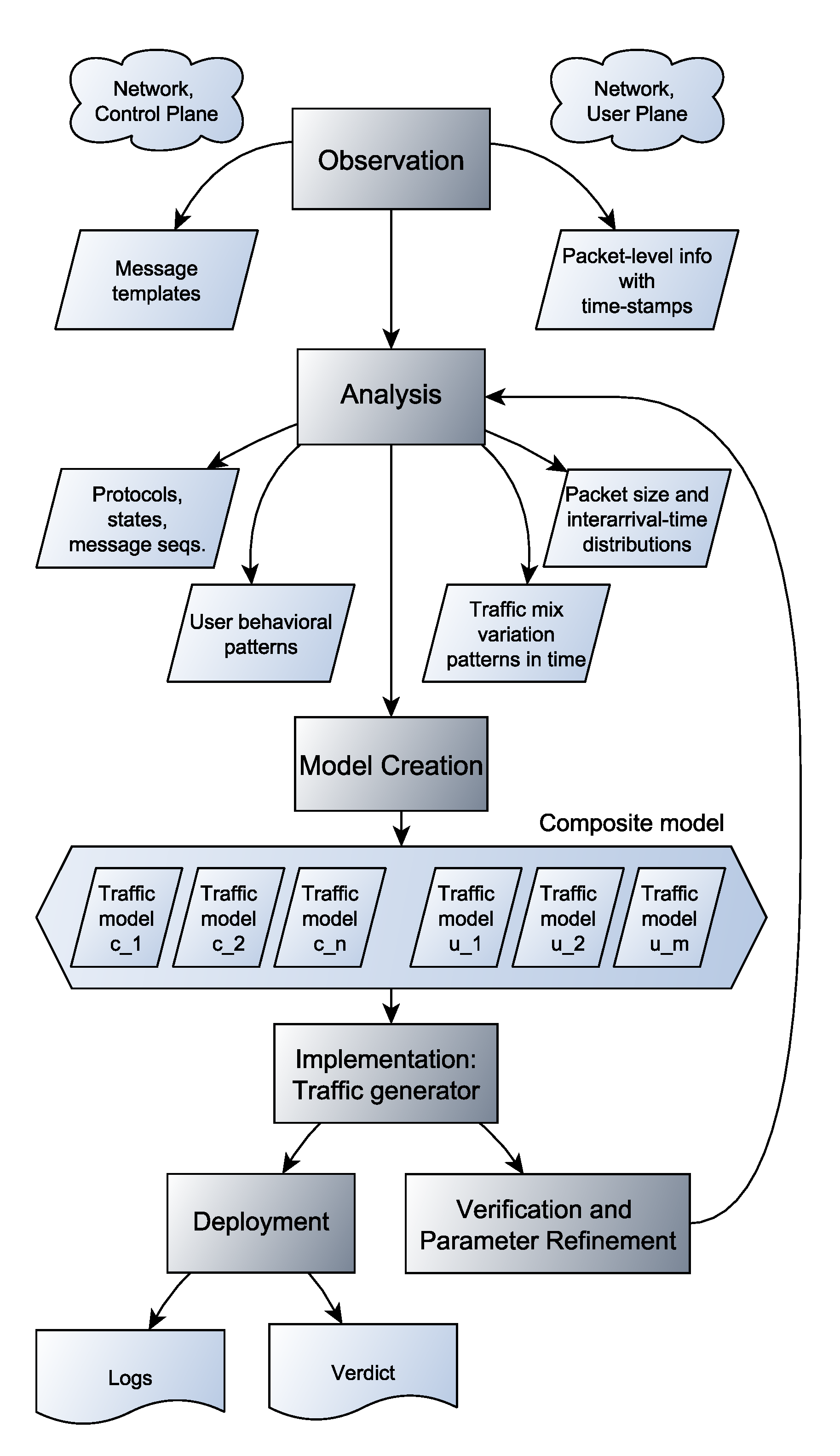
A major task of the methodology is traffic analysis, carried out in order to find proper models and parameters that fit this behavior. The models are implemented in the form of a traffic generator, which produces synthetic traffic whose statistical parameters match the observed real-life patterns. After verification and fine-tuning of the model, the traffic generator can be deployed in order to reveal the performance limitations of mobile core networks.

Figure 5 illustrates our methodology through the general cycle of modeling: observation, analysis, model creation, implementation and finally verification and deployment—according to [35].

• Observation: Capturing of real-life traffic data in an operational network. Traces are collected from both the control plane and the user plane.
• Analysis is performed on the collected data. Types of various network activities are identified. For each activity, relevant features and statistical parameters are identified, and their values are extracted from the data.
• Model creation: Based on the relevant parameters and message samples models are built, which account for the various activities and traffic patterns observed in the network.
• Implementation: The models are realized as a traffic generator. The device simulates the operation of a specific network segment through the parameters of the implemented models.
• Verification and refinement: The statistical properties of the synthetic traffic are matched against those observed in real patterns. The models’ parameters are refined in an iterative process in order to improve the prediction accuracy of the models.
• Deployment: Once the models are considered sufficiently accurate, the traffic generator can be deployed in a pilot network (or live network) to carry out complex load testing tasks. At this point the models may be operated outside the previously observed realistic parameter range. Thus the device can be used to simulate extreme network activities or boundary conditions, which would otherwise be difficult or impossible to produce in a real-life setup.

Because of their distinct characteristics, control and user planes need to be addressed separately throughout the model creation process.

4.1. Control Plane

Control plane messages are captured bit-by-bit. In the analysis phase, control message sequences and protocol state transitions are identified and stored. Subscriber mobility patterns are analyzed and their relevant parameters are identified.

The models created for the control plane are mainly based on protocol specifications: message sequences and state transitions need to conform to the standards and vendor-specific extensions. Subscriber mobility models, on the other hand, can as well employ statistical parameters.

4.2. User Plane

User plane capture is a process of collecting data packets sent over the network.

The analysis needs to identify categories of user activities – such as voice calls, video streaming, web browsing, email traffic, or IoT endpoint reporting periodically. The analysis also defines relevant parameters which characterize the activities (e.g. packet delay and jitter for VoIP and video; expected value and variance of packet sizes for email download).

Typically different sets of parameters (i.e., delay, jitter, loss rate) are identified for different types of observed activities (i.e., video streaming of IoT endpoint reporting).

4.3. Application of the Model for 4G Traffic-Based 5G Modeling

The next sections follow this methodology – by measurements and knowledge extraction (observation and analysis) on 4G live network traffic, and model creation, implementation on an experimental 5G network segment.

5. Analysis and Modeling of Current Mobile Network Traffic

After the mass launch of 3G and 4G smartphones and applications, the hunger for mobile data traffic has increased significantly. Mobile network operators were well aware that applications having video sharing functions, such as Youtube, Facebook, and Instagram would generate a high amount of data. Operators had developed different tariff packages in order to increase their revenues. The competition among SPs forced them to find out which applications and services are those that users most emotionally attached to. Previously, it was enough to determine about user groups how much data and when would they like to transmit, but this approach has been replaced by much more profound analytical methods. SPs were curious about which applications, websites are the most visited and when. This information is obtained through packet analysis (PA) and mainly used to meet business needs. Due to the evolving business requirements, researchers have made significant improvements in relation to traffic analysis and deep packet inspection (DPI). Nowadays, it is easy to provide a fair estimate about which application generated a specific network traffic flow – even for encrypted traffic.

5.1. Live Network Measurements

Regarding network design, the packet arrival rate and the size of data packets by a user or group of users have exceptional significance. In the Open Systems Interconnection Reference Model (OSI) L2 and L3 network layers switches, and routers are responsible for processing packet headers and deciding which direction to forward them. Received packets have to be saved in memory then forwarded to the chosen outgoing interface. This requires different sized buffers and transport tables. An L2 or L3 transmission device will react differently and transmit data packet at different speeds depending on their size. This paper does not cover the internal packet transfer properties of routers and switches, which are considered as Device or Network Under Test (DoNUT) and defined as a black box. By examining the inputs and outputs, conclusions can be drawn about the operation of the network and network elements [36].

One of the important features of Internet Protocol (IP)-based networks is that they can dynamically handle the traffic and traffic-directions. This flexibility and scalability also means that by analyzing traffic at a node, we can make estimations about the whole network traffic. From our analysis point of view, this is a disadvantage, since I would like to examine and draw conclusions separately for each upcoming use-case of 5G. To gather such accurate information, we have contacted one of the largest Internet providers in Hungary. The measurements were carried out within this service provider’s network. Measurements took place during September and October, 2019. Analyzing live network measurements is the best method to predict future traffic, even for cellular networks. By examining the current SP’s network, several conclusions can be presented regarding the live network traffic patterns, and general estimations can be made on the upcoming 5G traffic.

5.2. Identifying Application Types Based on Traffic Flows

The distributions of packet size and packet interarrival-time are essential parameters for the live network. Network operators aim to meet customer needs as quickly, efficiently, and properly as possible. In the previous section, we have shown that different usage demands require different packet size distributions and, thus, service requirements. However, the user experience, whether human or machine, is not necessarily the same as the packet size distribution.

If you are looking for a higher-level interpretation of customer experience, you might examine the network-side reactions to different kinds of user activities. For example, when a user opens a website, the time between sending the request and the arrival of the response, all of its related packages define a flow [37], which has a related user experience. Flows can be used to track the activity of a user or group of users. From another aspect, a flow can be a mixture of various traffic types (such as http or/and ftp samples) traversed between the same IP source/destination addresses and ports. This was already detailed in Section 2.

In a service provider’s DPI system, it is typically easy to separate anonymized user groups to different kinds of flows. Flows can be characterized by two parameters: the sum of transmitted data, and the total number of packets, where you can see how many packets have been handled by that flow. Of course, we can separate them to up- and downlink traffic as well.

The purpose of this paper is to provide models for the expected traffic types of future 5G use-cases through the identification of the essential properties of these traffic-types. The analysis takes place on a pre-5G network where the generated traffic approximates the traffic patterns of the identified application types. In order to draw the right conclusions and to make any predictions about the behavior of 5G applications, it is necessary to know the current mobile traffic trends. To determine what features eMBB, mIoT or cIoT will have, we need to know what trends are driving the current mobile networks.

In our previous work [38] we classified users based on their content nature into three categories. These categories – eMBB, mIoT and cIoT – already exist on 4G networks, as some kind of forerunner of future 5G use-cases.

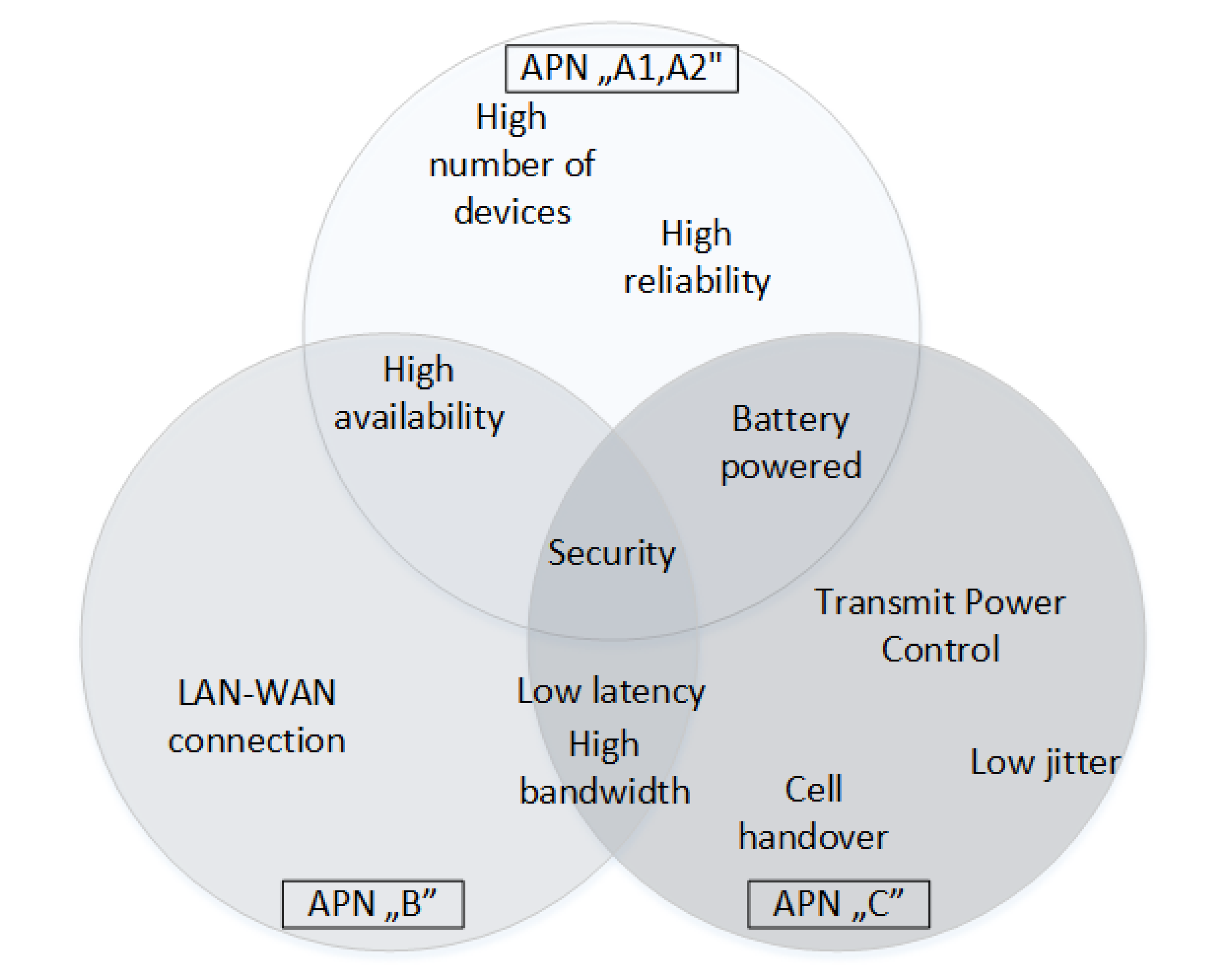
With 10 different features it can be described (see Figure 6) to which group a certain use-case belong to, and then identified these groupings within a live mobile network, where the subscription was bought by a service partner because their primary interest is these kinds of use-cases. With the help of Access Point Names (APNs), we examined these distinct user groups without their user identification. Although the exact borders of the three APNs can not be drawn precisely, the distinguishing features are shown in Figure 6 are more than enough for our examination. Nevertheless, strictly speaking, these forecasted 5G use-cases are not existing in current 4G networks; there are only groups with similar purpose can be found. Parts of the following brief description of APN scenarios are from our previous work [31].

We had the opportunity to monitor the traffic of a Hungarian SP, and its various APN’s traffic. There are certain traffic types that the operator aims to gather at given APNs. The traffic we analyzed was monitored in flow separation, each flow representing a user or user group experience. The APNs themselves are nationwide, so the random 10 000 sample is sufficiently representative, not too distorted by the habits of particular user groups. Regarding the analyzed user plane data, 10 000 flows were examined sequentially for each APN. Then, 10,000 packets were extracted from this 10 000 simultaneous flows and plotted. Regarding signalling – also for each APN –, 10,000 signalling messages were collected within a time-window, which we then processed. The report includes the number of packets of each flow and the total number of bytes per flow for up- and downlink on each APN.

For each APN, we plotted the size of the flows as a function of packet numbers. This method can be used to identify the traffic type that a given APN typically serves and the characteristic features that can be observed in traffic patterns. Also, we had prior knowledge about the type of traffic on each APN. For privacy reasons, we do not label each APN with their real name; it is not relevant to the content of this paper in what name they are called or to which service provider they belong.

5.2.1. mIot and cIoT as M2M Communication

APN “A1 and A2” serves mainly machine to machine type communication, as forerunners of mIoT and cIoT type use-cases. There are many subscriptions, with very-low-cost devices. The main business-case for the owners of such APNs are companies working with sensors of public services, or alarm devices of houses and cars. The user equipment (UE) sends keep-alive messages regularly, asking for status updates in a planned interval to one or more central server.

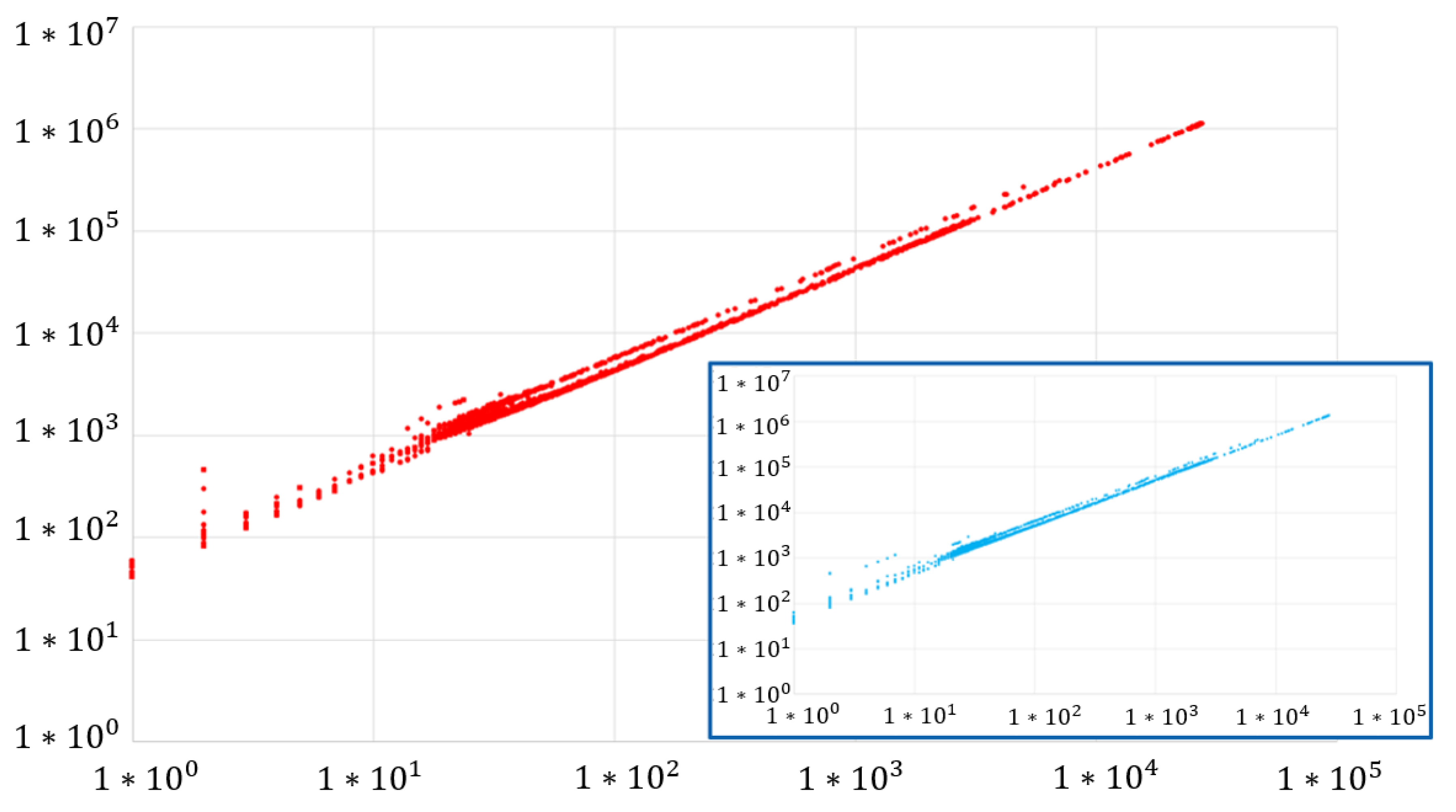
The APN “A1” traffic flows of downlink and uplink are shown in Figure 7, while APN “A2” in Figure 8. In these figures, a few “vertical line” can be seen, which represent specific events with a well-defined number of packets. This indicates that these APNs serve mainly M2M traffic. In the case of M2M applications, there are strictly defined transmission strategies, where the size and the number of packets sent by end-devices are determined.

5.2.2. eMBB as More Subscribers Behind Cellular Routers

APN “B” is a network segment connected by cellular routers [39]. Companies or individuals using these subscriptions to utilize one connection to the SP and then via network address translation (NAT) connect more local users via cable or WiFi. Main use-cases include surfing (web), communicating (e.g., Facebook, Skype), or watching online videos (e.g., YouTube). The owner of these subscriptions can use IP data tunneling between end subscriptions and centralized servers. Here the data consumers are mainly humans, but the operator of the devices connecting to a cellular network can be a company, not allowing the unnecessary reboot cycles. 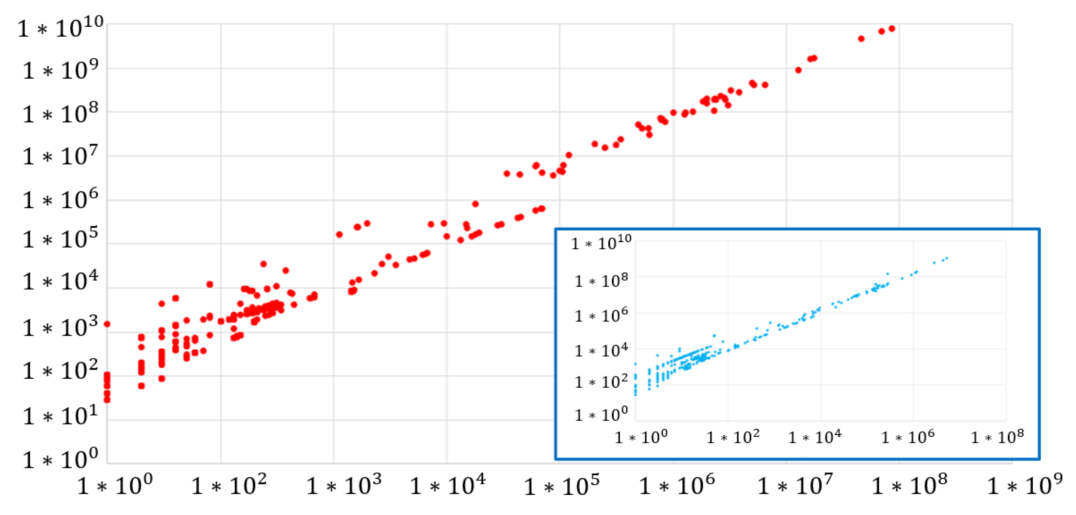Figure 9 shows the flow distribution of APN “B” traffic.

5.2.3. eMBB as Smartphone

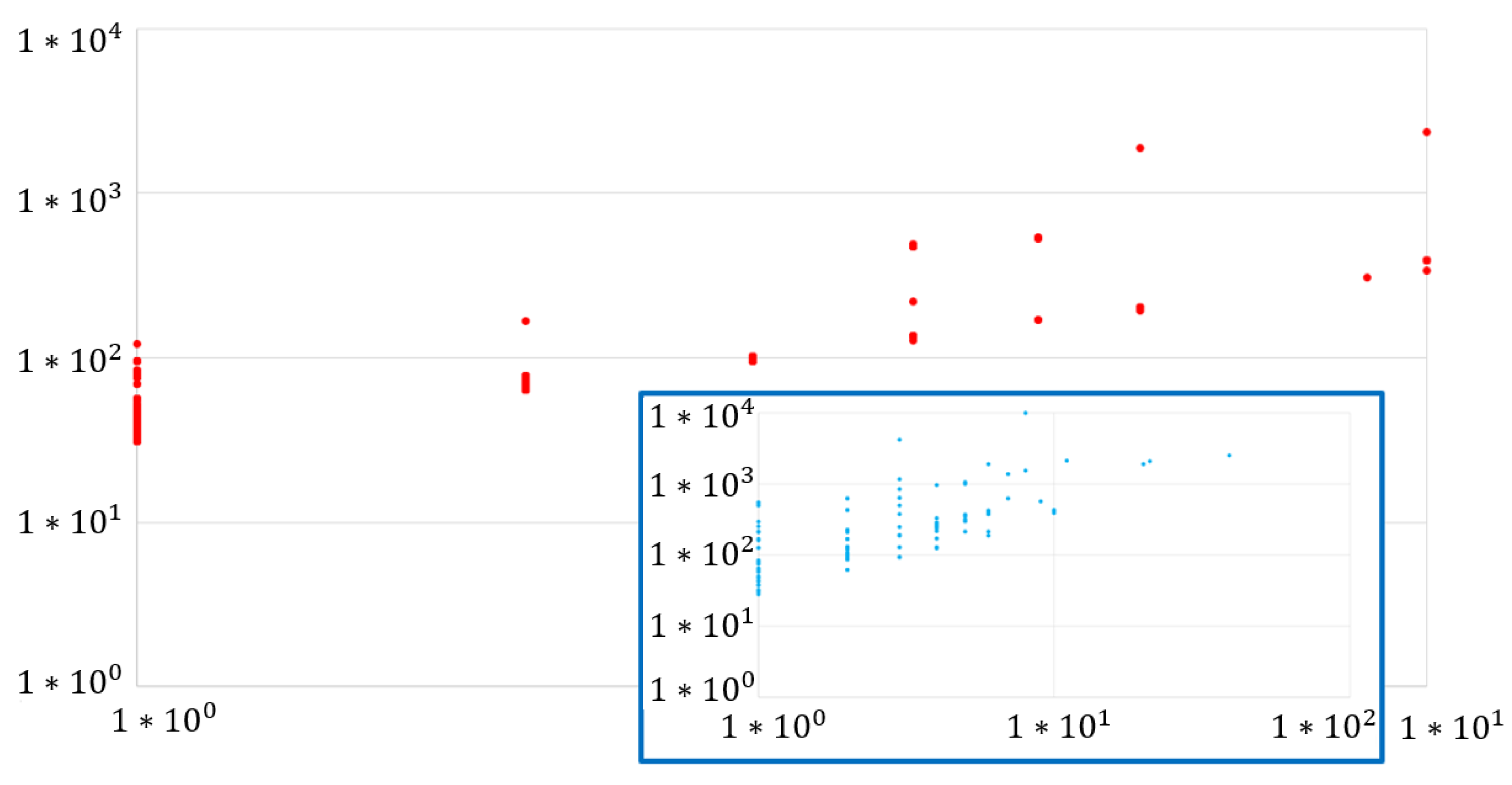
APN “C” is utilized by average cellular mobile subscribers: mainly smartphones, and universal serial bus (USB) sticks used by humans. These customers are also called mass-market at the SPs, who are selling these for anyone entering a customer representative shop. Based on the uplink and downlink traffic of the APNs in Figure 10 it can be seen that the flow sizes and the value of packet numbers are much more varied. It is clear that discrete lines are formed at certain packet numbers, each line is representing a specific event. The varied flow of traffic indicates that the APN “C” serving regular mobile users; thus, it is perfectly capable of simulating eMBB traffic.

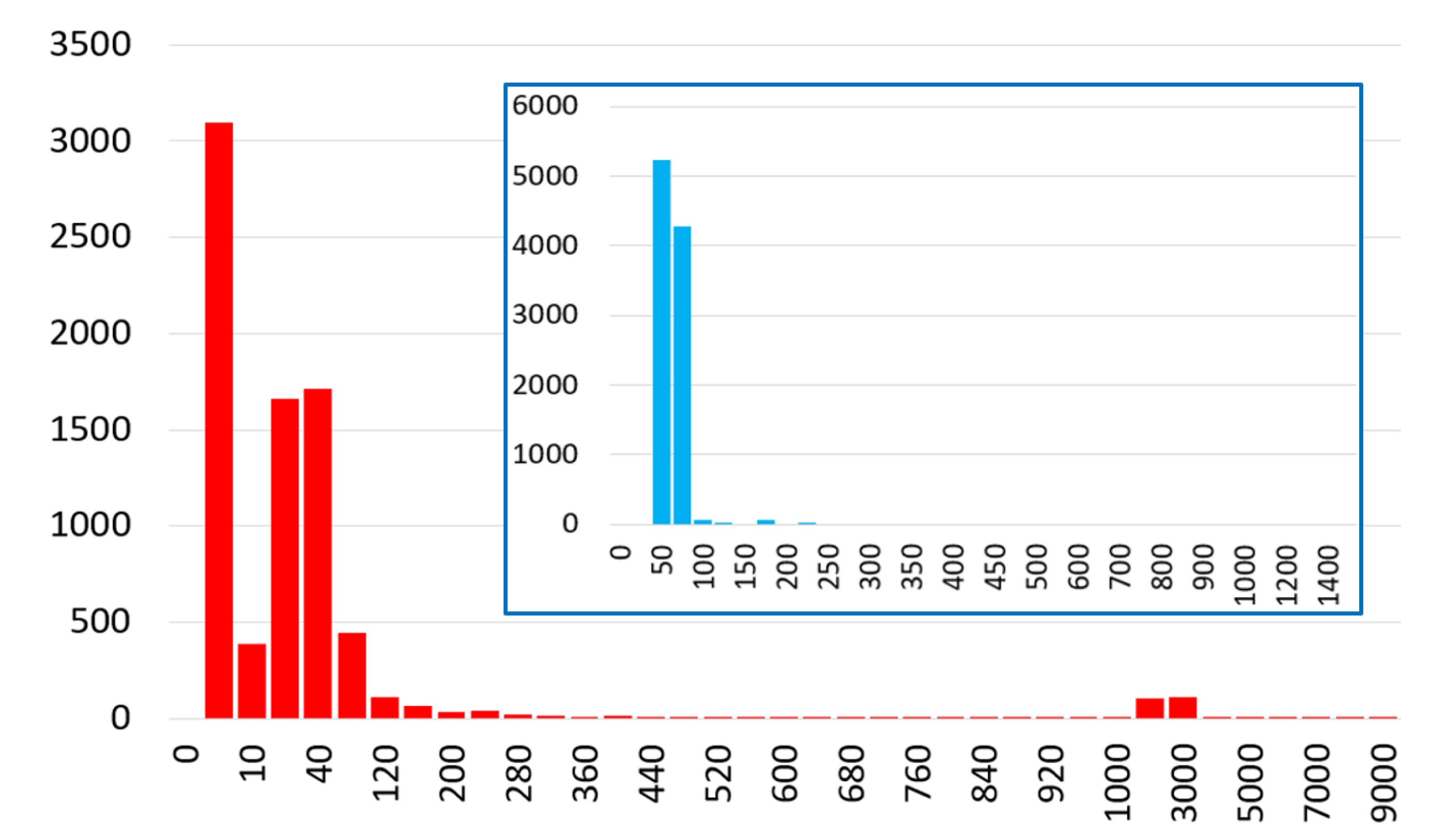
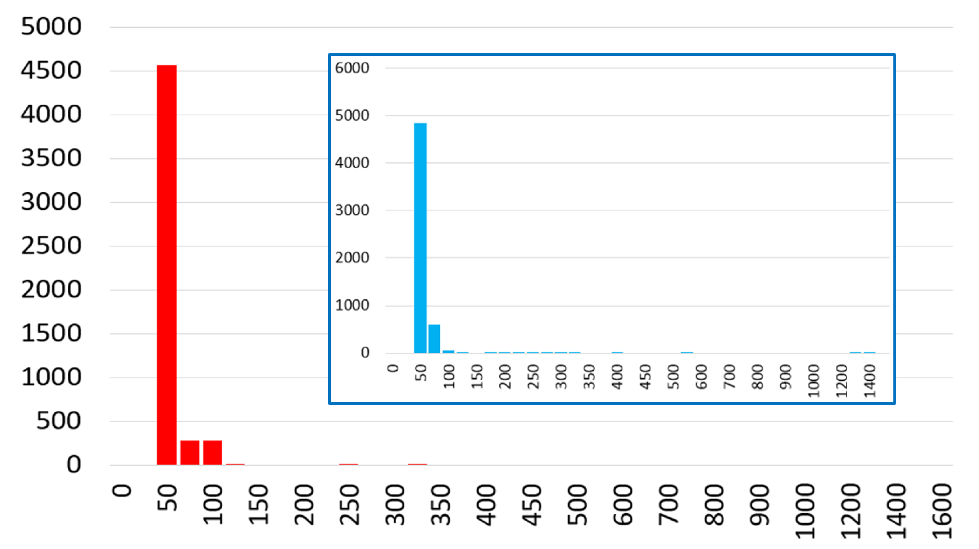
5.3. Identifying Application Types Based on Application Traffic Packet Size

To determine the different application traffic, we analyzed the measured traffic of the APNs on two different kinds of histograms. First, we examined the distribution of packet sizes of the flows (from Figure 11, Figure 12, Figure 13 and Figure 14). Second, we plotted the number of packets that each flow consists of (

Table 2. Flows packet size distribution on different APNs.

APN Name	Packet Size	Percentages
A1	50 Byte	89.10%
	75 Byte	5.5%
	100 Byte	5.4%
A2	50 Byte	84.62%
	75 Byte	15.38%
B	50 Byte	44.99%
	100 Byte	40.45%
	150 Byte	9.23%
C	150 Byte	69.56%
	375 Byte	13.03%
	600 Byte	10.8%
	1400 Byte	6.61%

and

Table 3. Flows packet number distribution on different APNs.

APN Name	Number of Packets	Percentages
A1	5	94.10%
A2	5	44.43%
	20	24.75%
	40	25.48%
B	5	92.58%
C	5	62.50%
	10	14.19%
	20	17.74%

). We have created both types of histograms in separate up- and downlink directions. These histograms approximate the density function of the packet numbers and packet sizes of the flows for each APN. Furthermore, they help to define the key parameters related to the discussed application-types traffic for the simulations. Once we have identified these parameters, the background traffic, and the application traffic types can be simulated.

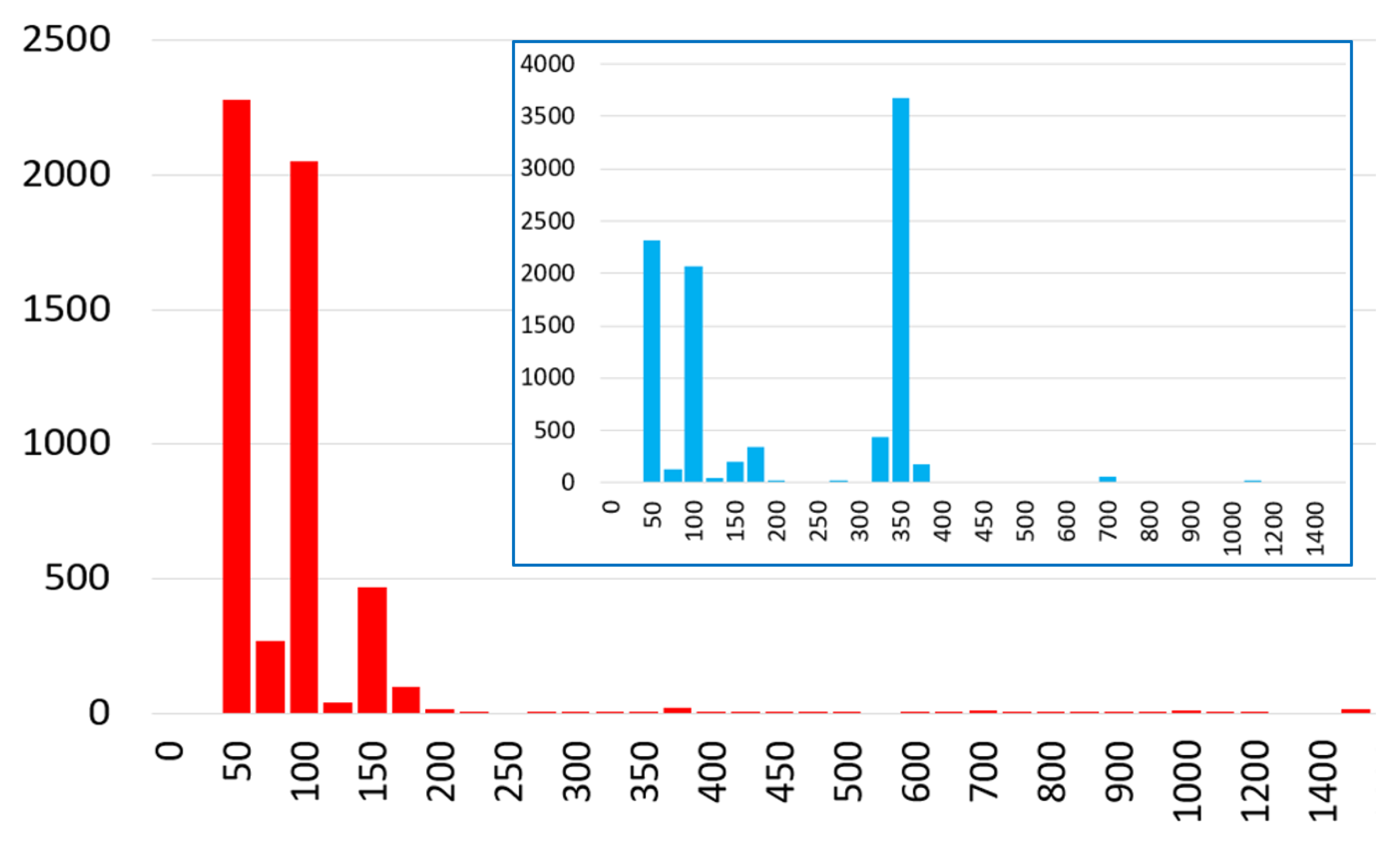
APN “A1”, APN “A2” and APN “B” can be used to model mIoT traffic. It can be observed that for APN “A1” and APN “A2”, the packet size distribution as shown in Table 2 can be derived from a single value (50 Bytes packets – Figure 11 and Figure 12) with a good approximation. APN “B” is a bit different from this pattern (Figure 13); there are significant numbers of 100 Bytes packets besides the 50 Bytes packets. For APN “A2” and APN “B”, the number of packets as shown in Figure 3 that create flow are between 0 and 5. The APN “A1” traffic is slightly different here, while the 5-packets flows are dominating the other two APNs’ traffic – APN “A2” and APN “B” –, here the 10 and 40 packet flows are also significant.

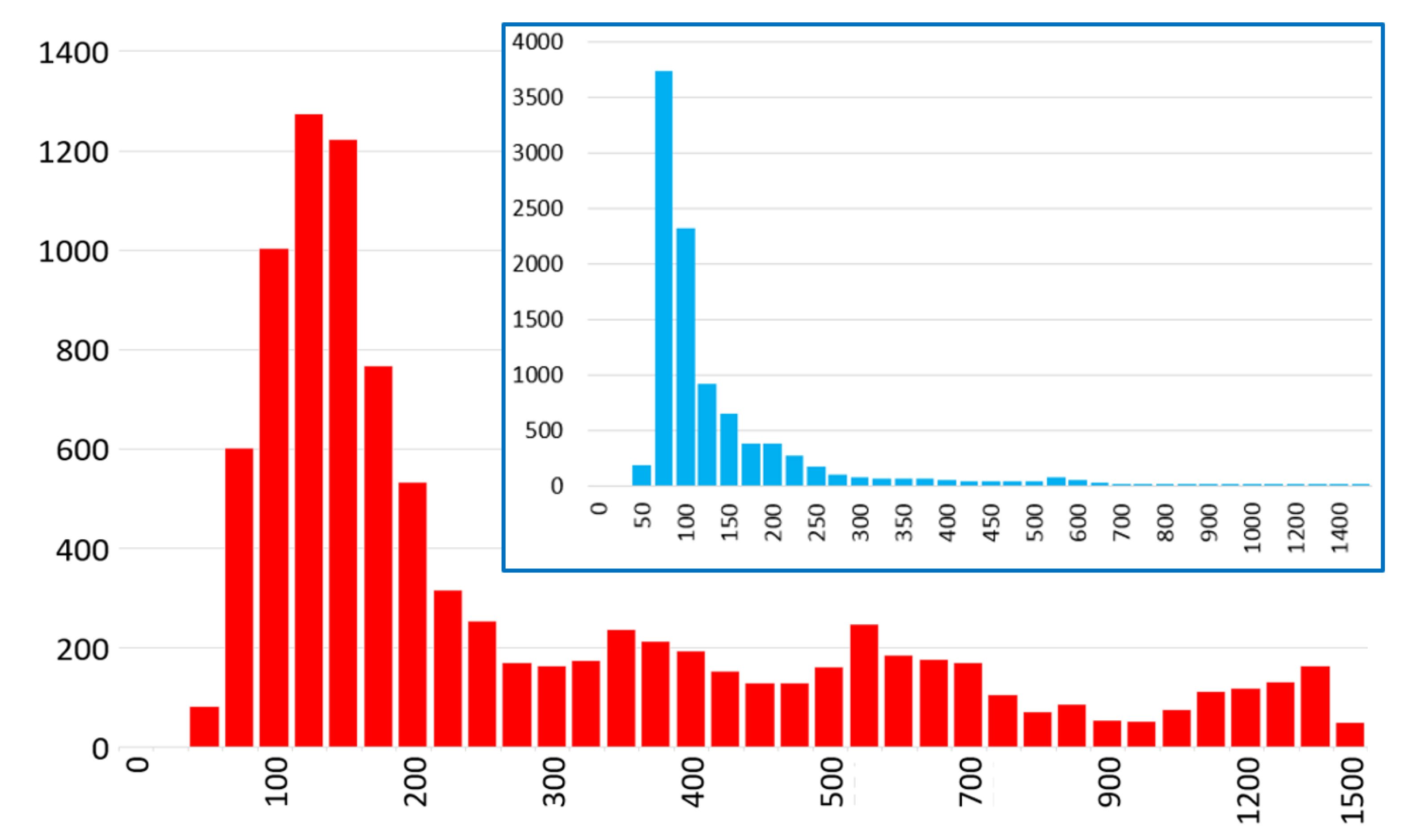
APN “C” traffic is used to model eMBB traffic (Figure 14). You can see that traffic on this APN cannot be modeled as easily as traffic on APN “A1”, “A2” and “B” (altogether: on mIoT). Here, the packet sizes that create the traffic are varied, unlike in the case of mIoT. There are fewer flows where the large packets are dominant, but this is not necessarily true in every scenario. For instance, Figure 13 shows an exception, where there is a peak at 350 Bytes, which typically refers to uplink IoT traffic. Flows with the usual shorter packets are more often seen in IoT traffic, but broadband traffic presents packets even larger than 1400 Bytes. For simpler modeling, we have identified the essential values of the packet size distribution and defined the modes (150, 375, 600, 1400 Byte). Based on these values, we have developed a traffic modeling function that seems to model the live network traffic according to my measurements accurately. However, it should be noted that this method may not always give an accurate approximation of live network traffic.

Note, that unfortunately, there are no real live representation of the cIoT traffic yet, as its significant benefits such as sub-ms latency and 99.99999% network availability can not be guaranteed at current mobile networks. Therefore, cIoT traffic is not to be included in our measurements. However, latency can still be measured, which is one of the essential requirements for these applications.

5.4. Identifying Application Types Based on Signaling Traffic Features

Analysis of signaling traffic is a common task at telecommunication operators [40]—and some assumptions from user traffic characteristics can also be extracted from these. PMR (Peak to Mean Ratio) is one of the best-known parameters for the interarrival times, useful for the operator to scale the system. In our case, we define the peak by two closest arrivals compared to the average arrival of events per second. The squared coefficient of variation (SCV) of the interarrival times is defined as $C^2\left(X\right)=Var\left(X\right)/E^2\left(X\right)$ where X is the interarrival time. Skewness is the third central moment (after mean and variance), and shows the asymmetry of the probability distribution, compared to a real random variable. The three statistics, PMR, SCV, and Skewness, are the basis for comparison of different traffic types. Our measurement results – previously published by us in [31] – for the given 72 h and for APN A, B and C are summarized in

Table 4. Basic statistical comparison of the APN characteristics.

APN	“A”	“B”	“C”
PMR	2859	4.85	121.8
SCV	137	1	4.73
Skewness	60	1.19	15.396

.

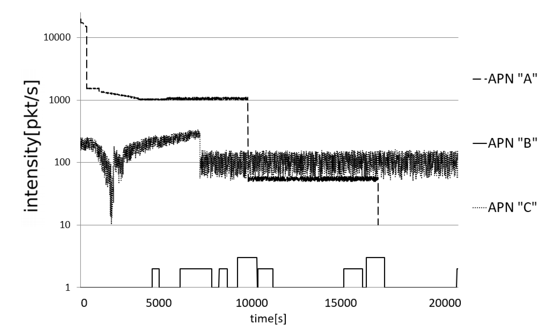
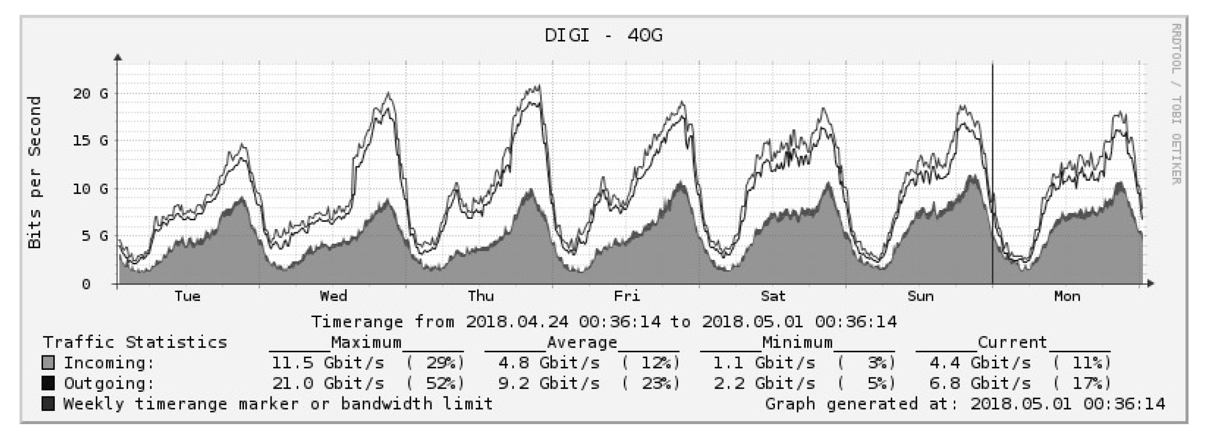
Intensity shows the number of arriving signaling packets correlating with time. Figure 15 shows the number of packets related to one second. This intensity view is very different from the well known data transmission figures, because the showed graphs are signaling traffic and not user data transport (which has trends shown in Figure 16). The differences between the use-cases are quite visible. Use-case APN A, as a machine-type device, requires very tight signaling traffic. The diagram shows a very clean change of the device’s behavior from the signaling point of view around 10,000 s. This also means that there are two different kinds of purposes these devices operate. On the other hand, the traffic of human operators in APN C is much more random. When applied in vast numbers, this will cause a more equalized signaling load, which is far better and more welcome on all server-side.

5.5. Packet Count Correlation for Signaling Traffic Types

To avoid server over-dimensioning and protect from bursty traffic, vendors usually apply queues on different links. This helps to decrease the bursts per server. However, if the bursty traffic gets repeated, the buffers will wobble continuously. To measure this undulation of traffic, the self interval packet count correlation will serve well. Figure 17 shows the great difference between the scenarios. Results for APN A show a huge self auto-correlation in the lag range of 0 to 200. Results for APN B show a lot of periodicity: the network signaling packet-count is relatively high among the users of this service. The APN C curve shows the characteristics of typical, human-originated usage.

6. Simulating Traffic Patterns

Earlier, we have shown the cellular networks’ main characteristics through two approaches. In Section 5.3, we have presented the packet distributions of the 4 examined APNs based on a passive measurement method. Then, we have shown what kinds of flow parameter value ranges can describe a given networking application – and its user experience. In this chapter, we examine how the user experience is affected in the different use-case scenarios by varying background traffic on a live 5G test network. To execute that, we create an active measurement set-up and generate the traffic flows based on the 4 different APNs traffic patterns. The measured 4G traffic was scaled up to the 5G data volume expectation. 5G networks are not used intensively yet, so it would not be relevant to make conclusions based on live 5G network traffic measurements.

6.1. Testbed Architecture

While building the testbed, we aimed to create a setup that resembles a live network architecture as much as possible. The layout is shown in Figure 18. Background traffic was generated by one device (UE2), and measurements were made with another client device (UE1). The UE1 is connected to the measurement server on one side and the Evolved Packet Core (EPC) on the other side via 4G and 5G base stations [41]. The EPC was then connected directly to the measurement server. It should be mentioned that the traffic in this set-up followed the 3GPP reference model 3.X [42], the traffic from the UE to the EPC used 4G devices, whereas downlink from the EPC to the UE used 5G network.

The UE2 generated the background traffic and used a wired connection. It is connected to the background traffic generator server’s client-side interface with a wired connection. UE2 is wirelessly connected to eNB and gNB, then it accessed the background traffic generator server, server-side interface via EPC.

The wired connections were 10 Gbps Ethernet in the testbed, which is similar to a live network. This way, our measurement can offer a good approximation to a live network scenario. With this architecture, those active parts of the network are examined, which influence the user experience the most. Measurements were carried out in a closed box, with set signal levels, under stable radio conditions for the measurement period – as suggested by [43,44].

6.2. Measurement Equipment

Measurement and Background traffic generator servers were x86-based machines with 12-core i7 processors, and had 8-8 GigaByte (GB) of memory. The network interfaces were Intel cards capable of real 4 × 2.5 Gbps Ethernet throughput on the client-side, while the server-side had 4 × 10 Gbps optical connections. The server traffic was provided by a software package based on Ubuntu 18.04. The major measurement, background traffic generator, and monitoring programs were the following: NMAP software packages [45], Iperf [46], Cisco T-rex [47], Ethernet, and Smooth ping. With the help of Iperf and T-rex, the background traffic was generated (packet size and rate), corresponding to Table 2 and Table 3. The network has been tested with Iperf and T-rex also to exclude burst measurement errors. After making sure that both led us to the same result, we presented only the measurement results of Iperf. We generated the measurement samples with Nmap. We used dedicated processor mapping and kernel compiled programs for the smooth running of the software. The measurement results were recorded for traceability purposes.

The EPC is a 2 × 64 × 86 server with 124 GB of memory and has a 2 × 10 Gbps link aggregation group (LAG) connection in all wired directions, towards Next generation NodeB (gNB) and Evolved Node B (eNB). The mobile network software consisted of 4G Mobility Management Entity (MME), Serving Gateway (SGW), Packet Data Network Gateway (PGW) with option 3.X architecture [48], where I implemented a minimal architecture design with only having the S6a interface outside of this. The system did not include any interface other than the minimal design.

The eNB and gNB were running in separate hardware (HW)s, with an x86-based architecture, dedicated with a 2 × 24 core processor and 8 GB of random access memory (RAM). The eNB was responsible for the 4G network, for the uplink channel and the controlling S1AP interface. It operated on 1.8 GHz band with 10 MHz bandwidth in 2 × 3 MIMO mode. The gNB operated on 3.6 GHz with 100 MHz bandwidth, but due to software limitations, it was safely used only in 2 × 2 MIMO mode. Clients were 2 × 3 MIMO mode devices conforming to the option 3.X architecture and were simultaneously connected to 4G and 5G networks. It was supported by a multi-core processor and several GBs of RAM. The brief technical details of the equipment with software versions involved in the tests are show in

Table 5. HW and SW description of devices in the testbed.

	Description
UE1 and UE2	Multicore Client Premise Equipment with dual 2.5GE interface, 8 × 8 Mimo
eNB as anchor cell	Uplink: 4G 64 QAM, Downlink: 256 QAM Radio at 1.8 GHz and 10 MHz Bandwidth, FDD
gNB	Downlink: 256 QAM, Radio at 3.6 GHz width 100 MHz Bandwidth, 64T64R antenna
EPC	Cisco C460 M2, 4x Intel Xeon E7-4870, supporting option 3.X
Measurement server	HP 360, 12x Intel Xeon E5649, 2x 10GE, 2x 2.5GE, Ubuntu 18.0.4 LTS
Background traffic	HP 360, 12x Intel Xeon E5649, 2x 10GE, 2x 2.5GE, Ubuntu 18.0.4 LTS, Cisco T-rex 2.66

.

6.3. Measurement Approach

The generic measurement setup has already been described by Figure 18. The main metrics to gather from our measurements are the different kinds of delays related to 4G and 5G network traffic. This delay-focused approach allowed us that the bandwidth and throughput of the two connecting users did not have to change over time, which also meant that there were no significant changes in relation to packet error rate or data loss in any of the scenarios.

The injected traffic consists of two main types. One is the background traffic, which aims to model the aggregated network traffic. The other type is the traffic of one single designated user or a group of users. While the amount of packets or bytes in a flow does not provide sufficient information when defining the background traffic, the distribution of packet sizes and the total number of bytes are the important parameters in this respect.

6.3.1. One-way Delay

In this setup the measurement traffic flows from the EPC interface of the measurement server to the EPC and then through the gNB via a wireless 5G connection to the UE1. Then, on the wired interface of UE1 there is a connection to the client-side interface of the measurement server.

6.3.2. Round Trip Time

In this setup the measured traffic flows from the UE-side interface of the measurement server to UE1 and then from UE1 to the eNB on a 4G radio access network. It accesses the measurement server from the eNB via the EPC via a wired connection. The measurement server records the arrival of packets and returns the data stream on its wired interface to the EPC. Passing through the EPC, it reaches gNB and then accesses the UE1 client device from the gNB via a 5G wireless connection. Finally, on the UE1 wired connection, it moves to the measurement server.

6.3.3. Perturbations due to Additional Background Traffic

The traffic of different application types was measured with different amounts of background traffic. The arbitrarily chosen measurement cases are as follows:

• without background traffic,
• 25% – of the available bandwidth – background traffic,
• 50% background traffic (to measure 1 direction latency),
• 100% background traffic.

Based in our measurements in Section 5.3, we identified the main flows’ and packet sizes in a typical cellular network. To describe the background traffic, we primarily considered traffic through the live network. However, we model the packet distribution composition of background traffic with APN “C”’s traffic as eMBB application-type traffic. This assumption is based on our previous analysis and previous work [49], where we have found that current machine-to-machine communication is negligible in volume compared to human communication. Furthermore, the predominant application-type (hence a significant portion of network traffic) will be eMBB traffic.

7. Results

The main parameters of the 5G testbed have been defined through a series of measurements, and for reference comparison, we have carried out similar measurements on 4G. The aggregated measurement results (

Table 6. Aggregated (median) results of measurements.

	4G - only	5G - 1 UE	5G - 2 UE
Downlink Peak Rate	420 Mbps	885 Mbps	1465 Mbps
Uplink Peak Rate	87 Mbps	92 Mbps	91 Mbps
Latency (one-way)	12 ms	3.71 ms	4.96 ms
Packet Error Rate	0.2%	0.39%	0.67%

) show that for 5G, even 1 UE downlink peak rate heavily outperforms the 4G values. However, 5G uplink transmission is an exception as it has similar performance as 4G. As expected, latency is also significantly lower at 5G than at 4G.

It was trivial that the basic bandwidth requirements would be fulfilled. However, by generating background traffic, we were able to examine the traffic correlated effects about latency and jitter, and the combined impact of different use-cases such as IoT, video and audio applications.

7.1. Detailed Latency Results

A key promise of 5G is that latency experienced with 4G will be reduced drastically to around 1 ms. Furthermore, latency can be kept low even if the traffic load is high in the network.

To measure 5G network latency in multiple scenarios, we examined how the DoNUT affects latency deviation. It was tested with different-sized packets and flows, where the packet-sending interval was between 25 ms and 200 ms.

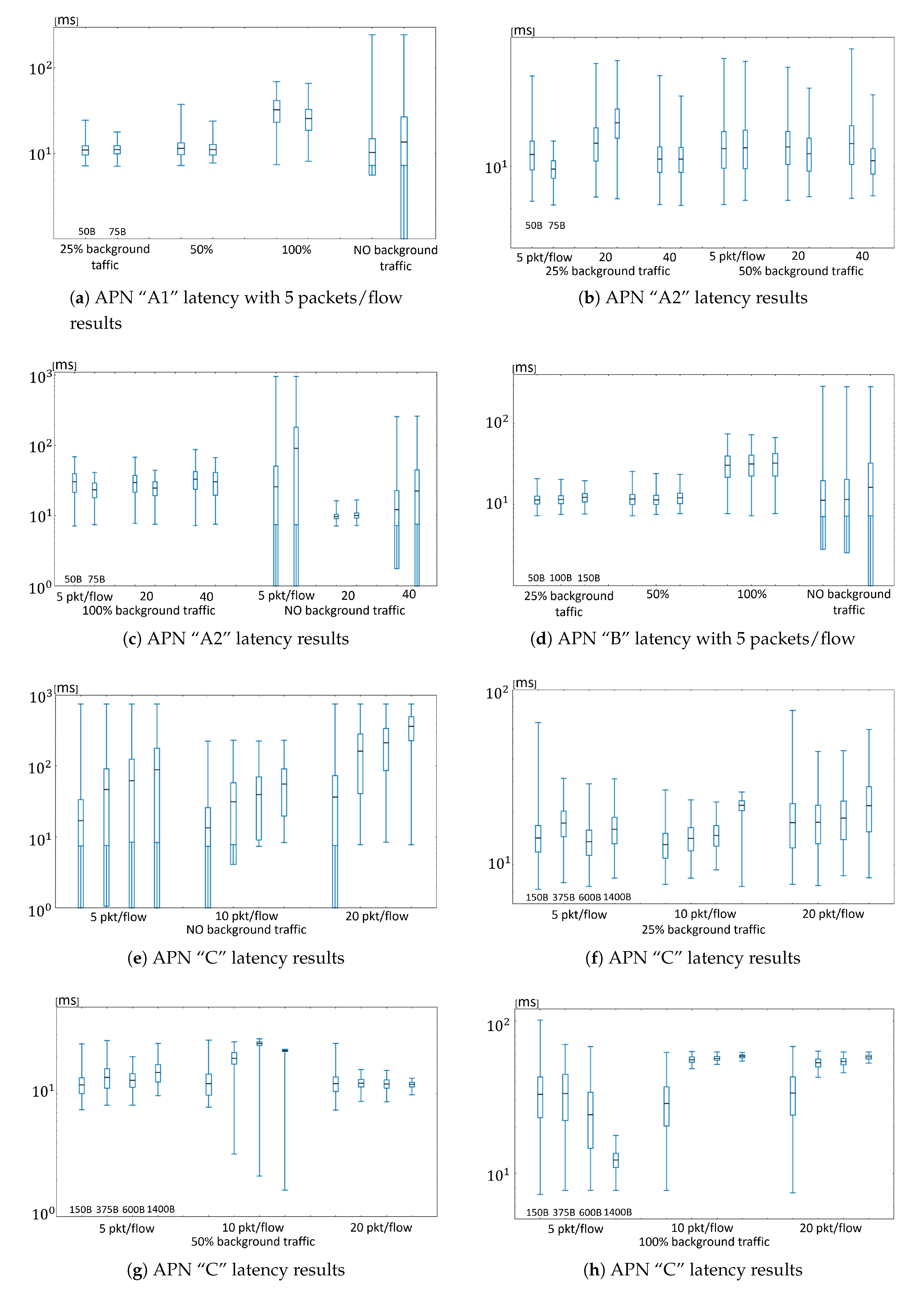
One-way latency results are depicted by Figure 19, where the measurement scenarios are based on our APN investigation results – the APNs are bonded with flow characteristics as shown on Table 2 and Table 3. The tests are perturbed with background traffic represented by the flows of APN “C”. The background traffic took multiple ratios from 0% to 100% of the link capacity. Again, Table 6 shows the aggregated results of the measurements.

As Figure 19 shows, the minimum values for the latency were relatively low, at all sending rates. Furthermore, the packet size does not really affect the minimum latency. The variance of the delay showed similar values for all measurement scenarios.

From Figure 19a–d we can see the user experience of “A1”, “A2” and “B” type APN-s. Since these traffic types are rather sterile – merely two kinds of packet sizes seem to appear –, their results do not differ that much. Minimum values are close to constant. The average values of latency grow when the cell is under high (background) load, although this growth is not extremely high; can be handled well by the applications.

Surprisingly, the observed variance without background traffic is much more significant. One possible explanation is that improving load balancing is one of the main goals of 5G. Because the examined 5G architecture is an early test deployment, this effect may change in the future. However, the packet numbers that make up the flows do not significantly affect the latency values; differences can be detected, but the measurement results do not show a clear pattern. From Figure 19b,c we can see that in case of larger packets the latency of the transmission is somewhat lower; however in case of larger scales as shown in Figure 19e, where the larger packets are almost 10 times larger than the smallest, although the latency is, of course, higher there.

In Figure 19h, where the measurement was taken with different transmission intervals and complex packet ratio, the maximum value of the latency has increased highly. It is especially interesting that the latency of sending bigger, 1000 Byte packets at each 100 ms shows smaller variance than the latency for 100 Byte packets at the same rate. This shows us that the DoNUT can handle the bigger-sized packets more smoothly.

Figure 19b,d,f,g depict our measurement results on different-sized packet-flows sent at different rates, where the background traffic was set to 25%. When taking a closer look at the maximum values of the packet-flow lengths, it seems that the network can handle the middle-sized flows smoothly. Interestingly the mean values of the latency did not change significantly throughout this scenario.

Figure 19g,h show measurement results, where significant – 50% and 100% – background traffic was put on the cell, respectively. There are various, interesting conclusions can be drawn by comparing the two figures. It is clear that the advantage of 5G networks is visible here: small packet flows are handled by the network with low latency. While the variance was low, latency sometimes reaches those very low, expected values of 5G—such as 3–4 ms. This does not increase much in the case of 100% background traffic, either. Figure 19e differs from these because there is no background traffic injected. The latency almost reached 1 s in a few occasions, but this was always due to the very first packet of the flow, which needed the radio channel to set up first.

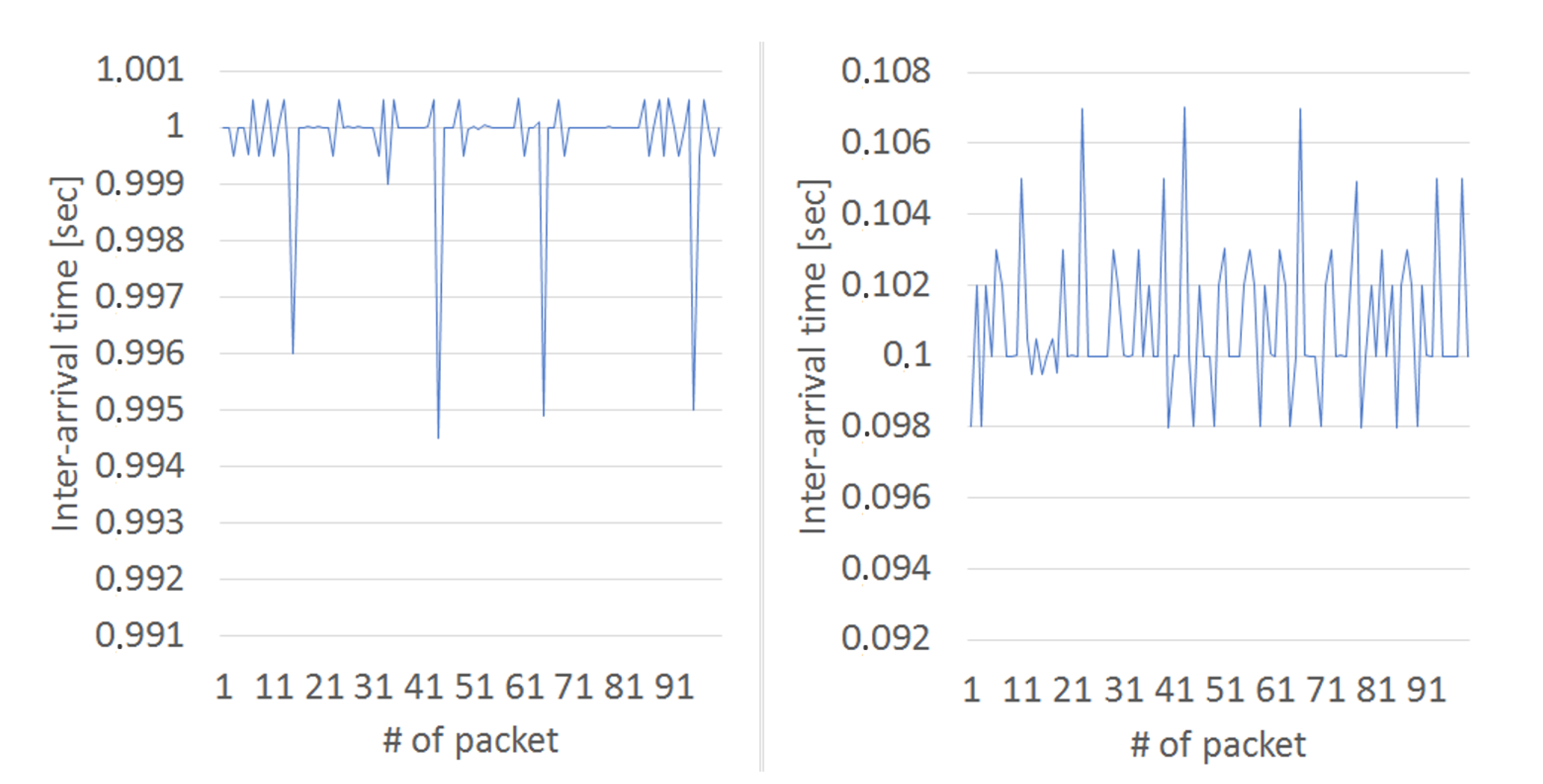
7.2. Detailed Jitter Results

In this measurement setup we were curious about the variance of the packet inter-arrival time during the transmission. The examined packets were 100 Bytes and 1000 Bytes long and also in 2 different packet sending interval scenarios between 1 and 0.1 s. Since we were controlling the ratio of packet sending in multiple dimensions, we also can calculate not only the variance of the packet arrival time, but also the variance difference between the expected and real arrival. The Equation (1) we used is very similar to calculating variance; however we replaced the mean “μ” to the packet sending interval as 1 s to 0.1 s. The absolute deviation around the expected packet arrival was also calculated with the Equation (2). Figure 20, Figure 21, Figure 22 and Figure 23 show the change of inter-arrival time in a graphical format. For comparison, we show all of the calculated results in

Table 7. Variance and absolute deviation around the expected packet arrival.

Dataset		100 Byte		1000 Byte
		1 sec	0.1 sec	1 sec	0.1 sec
without background traffic	${\sigma }^2{\left[msec\right]}^2$	0.0160618	0.232781	0.0222247	0.371
	$\xi$ [msec]	12.749	14.248	25.055	99.804
50% background traffic	${\sigma }^2{\left[msec\right]}^2$	0.01724	0.2157	0.0194	0.3426
	$\xi$ [msec]	11.617	14.155	18.665	67.493

. The variance is around 0.1 msec, and the highest deviation is 99.8 msec. Based on this we can state that our “Option 3x 5G testbed” provides very low jitter to the transmitted data even in case of high background traffic. Equations (1) and (2) we used is very similar to calculating variance and absolute deviation. To apply Equations (1) and (2), we replaced the mean “μ” with the packet sending interval as 1 s to 0.1 s, $x_i$ is the ith packet inter-arrival time; and n is the number of sent packets.

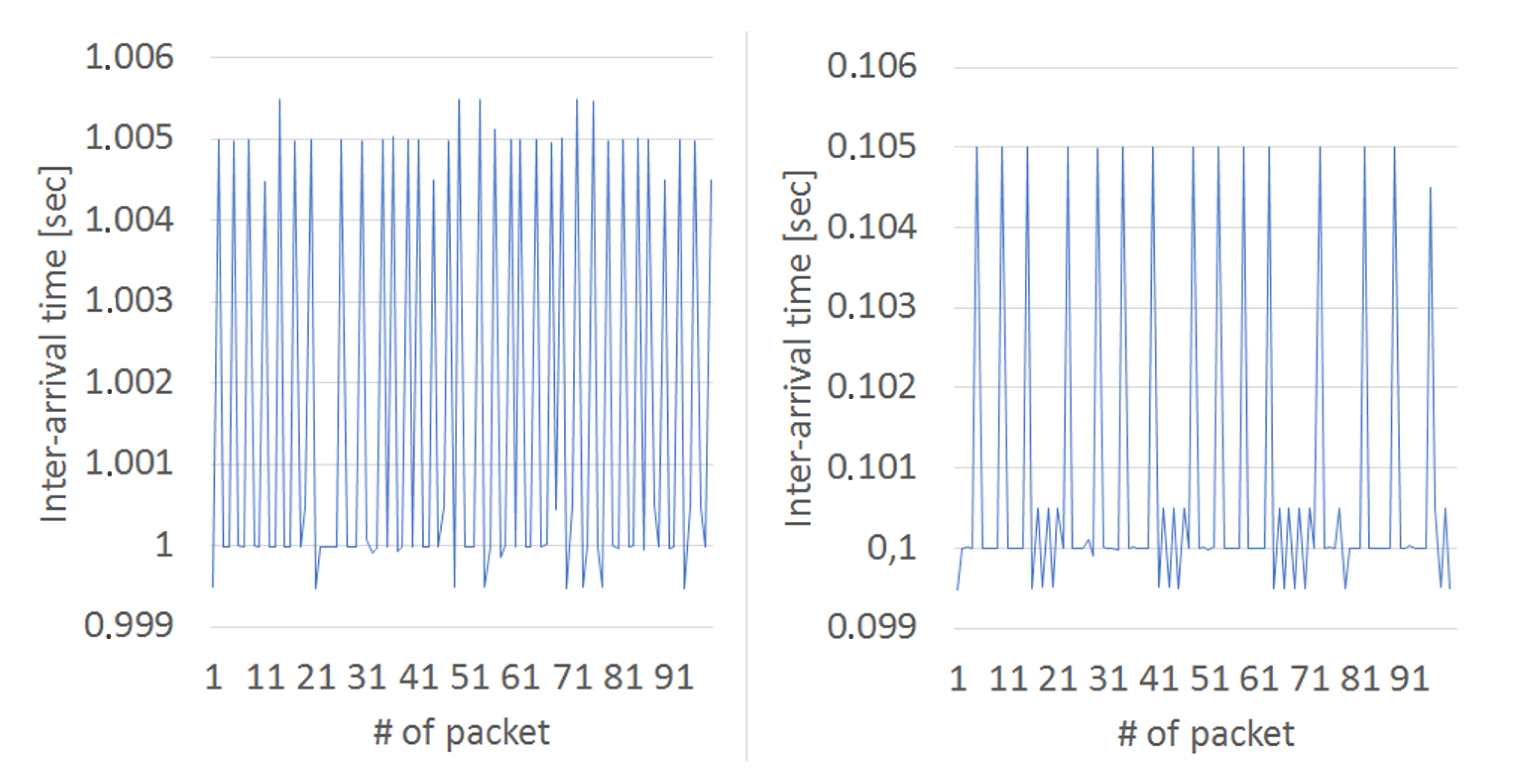
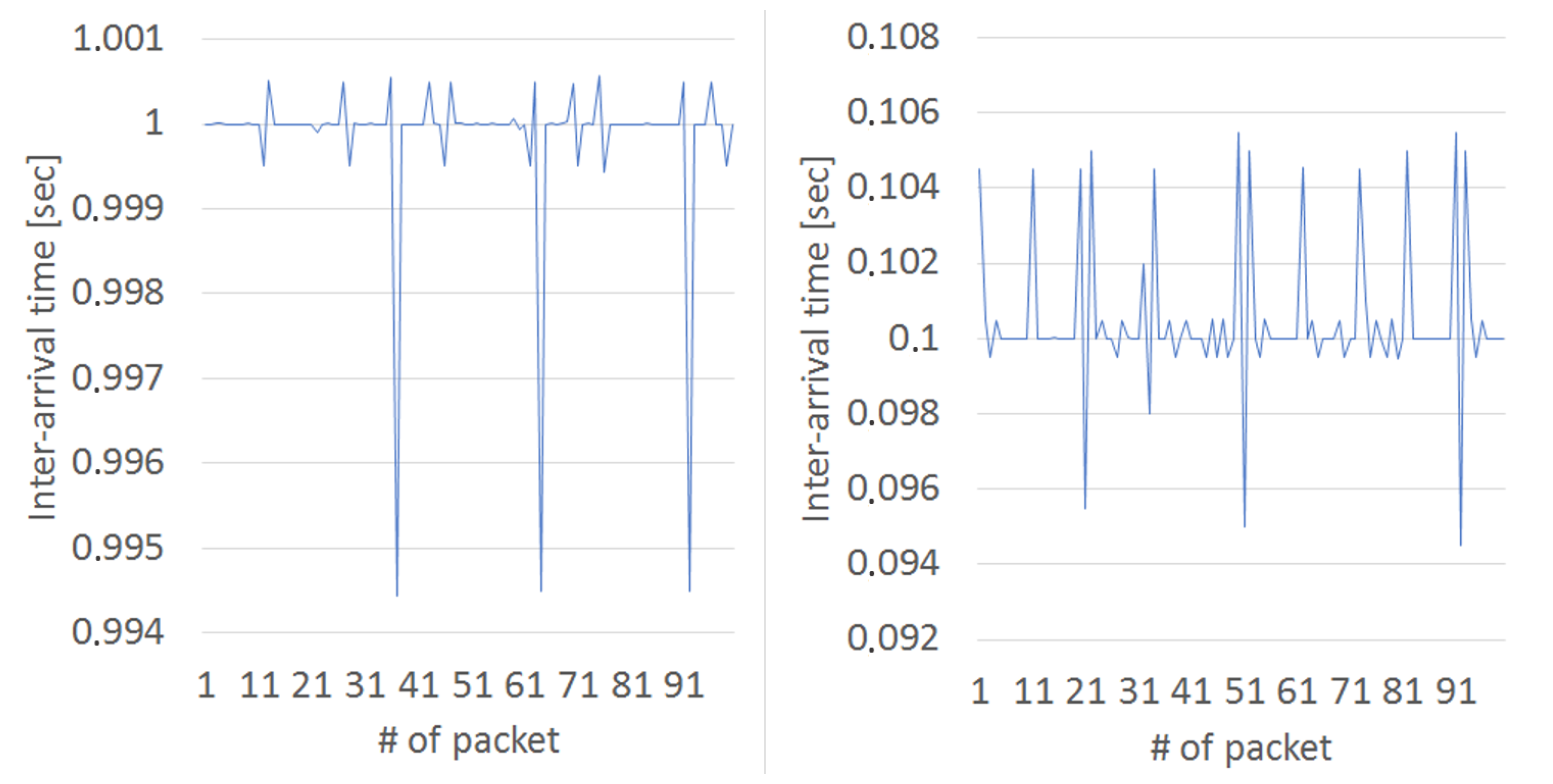
Figure 20 shows the received packets’ inter-arrival times with 0.1 and 1 s packet sending periods (in-between packets). The difference from the expected theoretical results is minimal. It is worth to mention that at 0.1 s packet sending period some packets arrive earlier occasionally. The reason could be the variance of transmission path latency. When examining the results of bigger packets’ transmission in Figure 21, we can see how 1000 Byte packets jitter changed during the test period. The received packets timestamp mostly differ from the reference in the negative direction. Specific channel allocation could be a reason for that. As a part of the 1000 Byte was transferred with the previous packet and the rest of them later.

$${\sigma }^2=\frac{{\sum }_{i=1}^n{(x_i-\mu )}^2}{n}$$

(1)

$$\xi =MAX\left|\right(x_i-\mu \left)\right|$$

(2)

Jitter Results With Background Traffic

During these measurements we wanted to examine how packet inter-arrival times vary in case of a loaded cell. To use the advantage of the DoNUT scenario we were also able to add background traffic in the earlier set radio and traffic data composition. Based on the previous measurements we knew that cell capacity is around 1400 Mbps, when Packet Error Ratio (PER) remains negligible, so we transmitted some background traffic during our latency measurement. The results are as follows.

Figure 22 has been created when the background traffic was arbitrarily set to 50% Mbps. When we compare these results with Figure 20, there is no considerable difference, except for a few packets.

The correlated effects of having 1000 Byte packets sent at various periodicity – without and with some background traffic – is shown by Figure 23. we can see that that neither latency nor jitter have changed drastically, even though the effect of cell load (due to the background traffic) is perceivable.

7.3. Lessons Learned Based on the Results

The aim of our paper was to provide a measurement methodology that can be used in practice by actual operators, who may want to compare their use-case performances with their expectations. This also means that the results presented are not supposed to be a baseline for further comparisons, but a snapshot of current status. Moreover, the idea behind comparing various use-cases was to show their differences, and not to universally answer the question of which use-case has better performance. This depends on the usage scenario, the volume of the traffic and masses how are using it.

Our measurement results showed that latency and jitter are still not significantly high for a fully-loaded cell, and the network will be able to fulfil the 5G mIoT and eMBB application use-cases requirements. There is no surprise that the latency of larger packets gets higher, but not proportionally with the packet length. For operators and network developers, we suggest to measure their benchmarks by using the suggested methodology and evaluate their network by using Equations (1) and (2) and compare their results as calculated in Table 7. These measurements with multiple packet lengths and send-intervals shall give enough space for correct network feature comparison and shall be used as KPIs.

We chose to demonstrate the extreme results of jitter in a general traffic case in order to show the best and worst case scenarios that the operator should take into consideration.

8. Conclusions

Through the identification and modeling of given application traffic types, this current work supports application developers and service providers in preparing traffic-related strategies for network slicing, together with better orchestration of the cellular core. Furthermore, from a quite opposite point of view, this work provides insight to characterizing traffic types that are the most suitable for the current hardware and software versions of the 5G network implementations.

An important part of our work is the refinement of the known methodology for interpreting network traffic not only as a sterile stream of packets of the same size and arrival rate but also for its diversity in arrival periodicity and packet sizes. As part of this refinement, besides the packet size distribution, we have defined the arrival frequency and the distribution of the data packet sets for a group of users. This correlates with the user experience of the subscribers for given application types. Describing this refined methodology, we have isolated, tested, and modeled user traffic similar to 5G use-cases. As a practical result, different application-types – including those eMBB, cIoT and mIoT that are distinguished for 5G – can be described using this method. The main parameters of the different use-cases were recorded and then fitted to the 5G network to investigate network effects. For measurement and model verification work, we have got to use various hardware and software elements:

• The mass user network management system for DPI measurements;
• 5G hardware and software equipment.

While analyzing the traffic of different application types, we have noted that applications used by people tend to use medium to large packets, where the up- and downlink directions show significantly different characteristics. The access network utilized merely by machines usually features traffic of small packet sizes with minimal or zero variance – for the up- and downlink, as well.

Based on this, we can conclude that our network should rather be optimized for fast transfer of small numbers of packets in a flow when the packet is received from the user – uplink. Depending on the traffic mix, the majority of the packets going to the user – downlink – are also small but there may be packets of a larger size and frequency. We used these results to model general background traffic in the network. Furthermore, it is a well known fact – and also seen from the measurement results – that the network transmits larger packets more easily, more efficiently.

Limitations during the measurements were experienced in both the User Equipment, Radio Access Network (RAN), and EPC network, since we were running early-released vendor-software. It was evident that there is still room for improvement at the software level on the 5G RAN. It is still worth noting that even by using such experimental software, we were able to achieve even better results in terms of service guarantees than those published in the current paper. However, they are not published here because such results can not always be achieved during standard operating mode. Furthermore, it was evident that the various client, RAN, or Core network software have not co-operate well in each case, thus significantly reducing the reliability of such (hence unpublished) measurement results. This, again, shows that there is room for improvement in 5G software capabilities.