Energy Storage Power and Energy Sizing and Specification Using HSSPFC

Abstract

The intermittent nature of renewable sources requires the integration of Energy Storage Systems (ESSs) with appropriate power and energy densities. One of the applications of Hamiltonian Surface Shaping and Power Flow Control (HSSPFC) is to size ESSs for power and energy densities by employing them as sole actuators of Microgrid (MG) systems. This Article provides a comprehensive yet simplified example of utilization of HSSPFC to size ESSs of inverter-based three-phase MG systems under hierarchical control. Here, the distributed Hamiltonian controller is expanded for control of parallel ESSs and power sharing metrics are defined to distribute power between hybrid storage systems according to their power and energy density capabilities. Simulated hybrid ESSs comprising battery and flywheel systems are used as examples to demonstrate the behaviour of the expanded control, verify the power sharing criteria and illustrate ESS design and specification by utilizing HSSPFC.

1. Introduction

From a design viewpoint, Energy Storage (ES) technologies need to be carefully chosen so that a suitable bandwidth of operation versus power transients is ensured. Long-term transients such as generation fluctuations over time-span of hours or days can be alleviated by using storage systems with high energy density such as batteries [1]. On the other hand, short-term transients such as load step changes may specifically require storage systems with high power density such as flywheels or super-capacitors [2]. The inherent benefits of these technologies can be combined to create a more capable hybrid storage system [3].

The Hamiltonian Surface Shaping and Power Flow Control (HSSPFC) method employs a multi-disciplinary approach to address stability and performance problems by providing solutions for power flow and energy transfer in various physical systems under control [4]. This work aims to illustrate how HSSPFC can be used for specification of battery and flywheel hybrid ESSs. One of the applications of the HSSPFC method is to obtain ES capacity and bandwidth requirements for dc and ac Microgrid (MG) systems [5,6,7,8]. The Hamiltonian control, unified in its original form is a centralized control method, however, decentralized and distributed solutions have been offered in recent works such as References [6,7,9] for dc, and Reference [8] for ac MG systems. From ES control and design perspectives, while Reference [6,8] provide solutions to obtain Energy Storage System (ESS) requirements, the Device Level Controllers (DLCs) have not yet been specified. In other words, it has not yet been shown how the end results interpret into sizing specific storage systems for capacity (energy density) and bandwidth (power density). Moreover, in References [6,8], a series combination of source and the ES element will have its specific limitations. Furthermore, ESS design and control using HSSPFC has not yet been instantiated for experimental implementation. This work aims to fill the gap between the rigorously analysed theoretical approach and the future device design and specification using the HSSPFC method.

The overall approach is to preserve the series form control from References [6,8] and define electrical levels for ES and the source systems so that the control laws for equivalent parallel form are derived. The series and parallel forms are equivalent in the power flow model defined by the HSSPFC [6]. Here, the control laws for parallel source and hybrid storage elements are derived to achieve two main objectives—first, to have an overall zero steady-state energy trade for the parallel ES elements, And second, to regulate the inverter dc voltage and reduce its variations versus source fluctuations. It will be shown that the corresponding ESS responses of each objective can be defined individually and stacked using superposition to form the overall storage control law.

Another purpose of this work is to demonstrate the efficacy of the HSSPFC method to control and specify battery and flywheel hybrid storage systems as actuators while maintaining electrical levels of the system. Here, reduced-order models for MGs in Reference [10], and battery and flywheel systems in Reference [11] are used. The renewable sources such as solar or wind are modeled as ideal variable voltage sources. It is also assumed that the average value of the variable source voltage is known. This is a major simplification of control design based on forecast. The purpose here is to demonstrate the functionality and capability of the developed control scheme for control design and find the minimum ESS capacity rather than finding the exact or optimum sizing value. Hence, the presented scenarios are developed to serve the requirements of the control scheme. Integration of solar or wind systems as well as control scenarios such as power curtailment [12], power smoothing [13], peak shaving [14], and MPPT [15] are left for future iterations of this work. Hereafter, the combinations of the reduced-order battery and flywheel models with their corresponding control systems are referred to as Battery Energy Storage Systems (BESSs) and Flywheel Energy Storage Systems (FESSs) respectively. By addressing BESS frequency response, the intent is the frequency response of the lumped battery with its control rather than the battery itself.

Parallel control of ESSs require appropriate power sharing criteria [16,17,18,19]. Considering the Low-Pass Filter (LPF) [20,21] nature of ESSs, References [16,17,18,19] use effective filter-based approaches to enable sharing of power. The simplicity and the hierarchical nature of this approach provides the motivation to use them for sizing hybrid ESSs using the HSSPFC. An alternative method for power sharing between ESSs is power-split based on power deviation [13]. In this case, the required power reference is smoothed by using a rate-limiter which is designed with respect to the controlled ESS. This approach leads to designing the rate-limiter according to the ramp-rate support capabilities of each storage device. While this algorithm-based approach is effective and can be implemented with ease, it does not consider the inherent LPF dynamic behavior of ESSs. Moreover, an algorithm-based approach limits the use of many conventional stability and performance analysis methods and tools. In this work, metrics are defined to design the BESS response as a portion of the RMS value of the reference power signal that is fed into the ESS control. It will be shown that accurate sizing of BESS for power density is possible by matching the responses of the BESSs to the splitting filter. Hence, for a system under hierarchical control, a hierarchical design approach for DLC appears to be a viable path to pursue.

This paper is organized as follows. First, the MG model in d-q coordinates is derived. In Section 3, the Hamiltonian control is developed. Section 4 elaborates on secondary and the primary distributed control. ESS control is discussed in Section 5. The details on ESS power and Energy sizing is given in Section 6 and the BESS/LPF matching and the overall design steps are shown in Section 7 and Section 8 respectively. Finally, illustrative examples are presented in Section 9.

2. Microgrid Model in DQ Coordinates

The MG system demonstrated in Figure 1 consists of a Distributed Generation Unit (DGU) connected to an RLC load [10]. The state-space model of the reduced-order MG with its inverter and ESSs was reformed according to the HSSPFC method. For the rest of this work, the combination of source, ESS, inverter and its filter/transmission line is referred to as the DGU or the local MG system. The state-space representation of the system demonstrated in Figure 1 is

$$\begin{array}{cc}\hfill L{\displaystyle \frac{d{i}_d}{dt}}& =-R{i}_d+\omega L{i}_q+v_d-v_{db}\hfill \end{array}$$

(1a)

$$\begin{array}{cc}\hfill L{\displaystyle \frac{d{i}_q}{dt}}& =-R{i}_q-\omega L{i}_d+v_q-v_{qb}\hfill \end{array}$$

(1b)

$$\begin{array}{cc}\hfill C_{dc}{\displaystyle \frac{d{v}_{dc}}{dt}}& ={\displaystyle \frac{(v+u-v_{dc})}{R_{dc}}}-\beta \lambda (cos\left(\varphi \right)i_d+sin\left(\varphi \right)i_q)\hfill \end{array}$$

(1c)

$$\begin{array}{cc}\hfill C_b{\displaystyle \frac{d{v}_{db}}{dt}}& =i_d+\omega C_b{v}_{qb}-i_{dLb}\hfill \end{array}$$

(1d)

$$\begin{array}{cc}\hfill C_b{\displaystyle \frac{d{v}_{qb}}{dt}}& =i_q-\omega C_b{v}_{db}-i_{qLb}\hfill \end{array}$$

(1e)

$$\begin{array}{cc}\hfill L_b{\displaystyle \frac{d{i}_{dLb}}{dt}}& =-R_b{i}_{dLb}+\omega L_b{i}_{qLb}+v_{db}\hfill \end{array}$$

(1f)

$$\begin{array}{cc}\hfill L_b{\displaystyle \frac{d{i}_{qLb}}{dt}}& =-R_b{i}_{qLb}-\omega L_b{i}_{dLb}+v_{qb},\hfill \end{array}$$

(1g)

where,

$$\left[\begin{array}{c}{v}_d\\ v_q\end{array}\right]=\beta \lambda v_{dc}\left[\begin{array}{c}cos\left(\varphi \right)\\ sin\left(\varphi \right)\end{array}\right].$$

(2)

The compact HSSPFC representation is

$$\begin{array}{ccc}\hfill \mathit{M}\dot{\mathit{x}}& =\mathit{R}\mathit{x}+{\mathit{B}}^{\mathit{T}}\mathit{u}+{\mathit{D}}^{\mathit{T}}\mathit{v},\hfill & \hfill \end{array}$$

(3)

where,

$$\begin{array}{cc}\hfill \mathit{x}& ={\left[i_d{i}_q{v}_{dc}{v}_{db}{v}_{qb}{i}_{dLb}{i}_{qLb}\right]}^T\hfill \end{array}$$

(4a)

$$\begin{array}{cc}\hfill \mathit{u}& =u\hfill \end{array}$$

(4b)

$$\begin{array}{cc}\hfill \mathit{v}& =v,\hfill \end{array}$$

(4c)

and,

$$\begin{array}{c}\hfill \mathit{M}=\left[\begin{array}{ccccccc}L& 0& 0& 0& 0& 0& 0\\ 0& L& 0& 0& 0& 0& 0\\ 0& 0& C_{dc}& 0& 0& 0& 0\\ 0& 0& 0& C_b& 0& 0& 0\\ 0& 0& 0& 0& C_b& 0& 0\\ 0& 0& 0& 0& 0& Lb& 0\\ 0& 0& 0& 0& 0& 0& Lb\end{array}\right],\end{array}$$

(5)

$$\begin{array}{c}\hfill \mathit{R}=\left[\begin{array}{ccccccc}-R& \omega L& \beta \lambda cos\varphi & -1& 0& 0& 0\\ -\omega L& -R& \beta \lambda sin\varphi & 0& -1& 0& 0\\ -\beta \lambda cos\varphi & -\beta \lambda sin\varphi & -1/R_{dc}& 0& 0& 0& 0\\ 1& 0& 0& 0& \omega C_b& -1& 0\\ 0& 1& 0& -\omega C_b& 0& 0& -1\\ 0& 0& 0& 1& 0& -R_b& \omega L_b\\ 0& 0& 0& 0& 1& -\omega L_b& -R_b\end{array}\right],\end{array}$$

(6)

$$\begin{array}{cc}\hfill {\mathit{B}}^{\mathit{T}}& ={\left[00{\displaystyle \frac{1}{R_{dc}}}0000\right]}^T,\hfill \end{array}$$

(7)

$$\begin{array}{cc}\hfill {\mathit{D}}^{\mathit{T}}& ={\left[00{\displaystyle \frac{1}{R_{dc}}}0000\right]}^T.\hfill \end{array}$$

(8)

This system can further be analyzed for stability and performance using the HSSPFC [4,5,6]. A single DGU connected to a load was presented for the sake of simplicity, however, there are typically multiple DGUs in a MG system. In Section 4, a d-q droop control [22] will be be leveraged for sharing the load power between parallel DGUs in a distributed form. In the next sections, the overall control systems will be derived based on the model that was presented in Figure 1.

3. Hamiltonian Control Derivations for Parallel Hybrid Storage Systems

The reference state-space of the system in Figure 1 is obtained as below,

$$\begin{array}{ccc}\hfill \mathit{M}{\dot{\mathit{x}}}_{\mathit{ref}}& =\mathit{R}{\mathit{x}}_{\mathit{ref}}+{\mathit{B}}^{\mathit{T}}{\mathit{u}}_{\mathit{ref}}+{\mathit{D}}^{\mathit{T}}\mathit{v}.\hfill & \hfill \end{array}$$

(9)

This expression consists of reference, nominal and measured values. The feed-forward control expressions for ES and inverter command controls are obtained from the steady-state solution of this reference state-space system. In this section, the ES feed-forward and feedback, and inverter feed-forward control laws for parallel sources and ESSs are obtained.

The series combination of the ES element u with the source voltage v might not always be equivalent to parallel form since at some operation points internal currents may flow between the two components. In this case, the parallel equivalent model would not be feasible. Moreover, in the series topology, ES element might limit the current supply of the source, and introduce more complexity such as requirement of high-side driving for converter control. In this section, the parallel form of the combined source and ESS is realized from the baseline series form. The general aim is to develop control laws for the ES element to satisfy specific constraints. Ideally, the effects of each constraint on ES element can be identified and eventually stacked using superposition principle to obtain the overall ES requirements. Here, the parallel ESS actuator is constrained to include zero steady-state response for the ES element and regulate the inverter dc-input voltage $v_{dc}$. The inverter dc-input reference voltage denoted by $v_{dc,ref}$ will be used to enable the Hamiltonian controller to determine the ES requirements.

Considering (9), corresponding error state is

$$\begin{array}{cc}\hfill \tilde{\mathit{x}}& ={\mathit{x}}_{\mathit{ref}}-\mathit{x}.\hfill \end{array}$$

(10)

For the system in (1), the error is defined as

$$\begin{array}{cc}\hfill e& =v_{dc,ref}-v_{dc}.\hfill \end{array}$$

(11)

Therefore, the ES PI feedback is

$$\begin{array}{cc}\hfill \Delta u& =-k_{p}e-k_i{\int }_0^{t}ed\tau ,\hfill \end{array}$$

(12)

and the ES feed-forward is

$$\begin{array}{cc}\hfill u_{ref}=& R_{dc}\beta \lambda (cos\left(\varphi \right)i_{d,ref}+sin\left(\varphi \right)i_{q,ref})-v+v_{dc,ref}.\hfill \end{array}$$

(13)

Hence, the overall ES feed-forward and feedback control law for the series form in (1) is

$$\begin{array}{cc}\hfill u& =u_{ref}-\Delta u\hfill \\ \hfill & =R_{dc}\beta \lambda (cos\left(\varphi \right)i_{d,ref}+sin\left(\varphi \right)i_{q,ref})-v+v_{dc,ref}\hfill \\ \hfill & +k_{p}e+k_i{\int }_0^{t}ed\tau .\hfill \end{array}$$

(14)

The series topology of v and u can be obtained from the parallel form and vice versa according to Reference [6] so that

$$\begin{array}{cc}\hfill v& ={\displaystyle \frac{R_u}{R_u+R_v}}{v}_v\hfill \end{array}$$

(15a)

$$\begin{array}{cc}\hfill u& ={\displaystyle \frac{R_v}{R_u+R_v}}{u}_u\hfill \end{array}$$

(15b)

$$\begin{array}{cc}\hfill R_{dc}& ={\displaystyle \frac{R_u{R}_v}{R_u+R_v}}\hfill \end{array}$$

(15c)

$$\begin{array}{cc}\hfill i_u& ={\displaystyle \frac{u_u-v_{dc}}{R_u}}\hfill \end{array}$$

(15d)

$$\begin{array}{cc}\hfill i_v& ={\displaystyle \frac{v_v-v_{dc}}{R_v}},\hfill \end{array}$$

(15e)

where, $v_v$ and $u_u$ represent the energy source and storage device for the parallel form. $i_v$, $i_u,$$R_v$ and $R_u$ are the corresponding currents and resistances. The objective is to keep $i_u$ at zero level at steady-state then superimpose the requirements to maintain a constant $v_{dc}$ versus the change in the input source $v_v$.

To have a zero $i_u$, $u_u$ should satisfy

$$\begin{array}{cc}\hfill {\displaystyle \frac{u_u-v_{dc}}{R_{dc}}}& =i_u=0,\hfill \end{array}$$

(16)

from which the series form response for u can be obtained as

$$\begin{array}{c}\hfill u_1={\displaystyle \frac{R_v}{R_u+R_v}}{v}_{dc}.\end{array}$$

(17)

Assuming $v_{v,avg}$ is the average value of the source voltage $v_v$, the dc error $e_{dc}$ can be defined as

$$\begin{array}{cc}\hfill e_{dc,v}& =v_v-v_{v,avg}.\hfill \end{array}$$

(18)

Considering (15), in series form, this error can be scaled to

$$\begin{array}{cc}\hfill e_{dc}& ={\displaystyle \frac{R_u}{R_u+R_v}}{e}_{dc,v}=v-v_{avg}.\hfill \end{array}$$

(19)

To remove and compensate for $e_{dc}$, the ES element u in (14) can be set to

$$\begin{array}{cc}\hfill u_2\left(t\right)& =-e_{dc}.\hfill \end{array}$$

(20)

From above, $u_1$ and $u_2$ are the required responses for u to satisfy the constraints in (16) and (10). Using superposition, from (17) and (20), the overall lumped u should satisfy

$$\begin{array}{c}\hfill u_{1,2}={\displaystyle \frac{R_v}{R_u+R_v}}{v}_{dc}-e_{dc}.\end{array}$$

(21)

To enforce the above equation, from (13), $v_{dc,ref}$ can be set to

$$\begin{array}{cc}\hfill v_{dc,ref}& =v+u_{1,2}-R_{dc}\beta \lambda (cos\left(\varphi \right)i_{d,ref}+sin\left(\varphi \right)i_{q,ref})\hfill \\ \hfill & =v_{avg}+{\displaystyle \frac{R_v}{R_u+R_v}}{v}_{dc}\hfill \\ \hfill & -R_{dc}\beta \lambda (cos\left(\varphi \right)i_{d,ref}+sin\left(\varphi \right)i_{q,ref}).\hfill \end{array}$$

(22)

For overall ES control, from (15), $u_u$ is controlled according to

$$\begin{array}{c}\hfill u_u={\displaystyle \frac{R_u+R_v}{R_v}}u,\end{array}$$

(23)

or $i_u$ can be controlled according to

$$\begin{array}{c}\hfill i_u={\displaystyle \frac{u_u-v_{dc}}{R_{dc}}}.\end{array}$$

(24)

Hence, for a current-controlled storage system, the overall ES command is

$$\begin{array}{cc}\hfill i_u& ={\displaystyle \frac{{(R_u+R_v)}^2}{R_v^2{R}_u}}u-{\displaystyle \frac{R_u+R_v}{R_v{R}_u}}{v}_{dc},\hfill \end{array}$$

(25)

where, u is obtained from (14) and $v_{dc}$ is the measured dc bus voltage.

4. Primary and Secondary Control Derivations

4.1. Primary Control System: DQ Droop Control

The d-q droop control [22] as the primary controller for the source MG in Figure 1 is given as

$$\begin{array}{cc}\hfill I_{d,i}& ={\displaystyle \frac{V_{d,i}^{*}-V_{db}}{R_{d,i}}}\hfill \end{array}$$

(26a)

$$\begin{array}{cc}\hfill I_{q,i}& ={\displaystyle \frac{V_{q,i}^{*}-V_{qb}}{R_{q,i}}}.\hfill \end{array}$$

(26b)

where, $V_{d,i}^{*}$ and $V_{q,i}^{*}$ are the droop voltage settings. $R_{d,i}$ and $R_{q,i}$ are the droop slope settings. $I_{d,i}$ and $I_{q,i}$ are the corresponding currents injected into d-q buses. $V_{db}$ and $V_{qb}$ are the measured bus d-q voltages.

If $I_d$ and $I_q$ are determined, the real and reactive powers, P and Q can be obtained according to

$$\begin{array}{cc}\hfill P_i=& V_{db}{I}_{d,i}+V_{qb}{I}_{q,i}\hfill \end{array}$$

(27a)

$$\begin{array}{cc}\hfill Q_i=& V_{qb}{I}_{d,i}-V_{db}{I}_{q,i}.\hfill \end{array}$$

(27b)

The droop settings $V_{d,i}^{*}$, $V_{q,i}^{*}$, $R_{d,i}$ and $R_{q,i}$ are obtained from a secondary controller to improve regulation of $V_{db}$ and $V_{qb}$ which represent the three-phase bus voltage.

4.2. Secondary Control System: Power Flow Calculations

Droop control in (26) can operate without communication and load information however, the bus voltage may suffer for lack of communication for long duration of time. A secondary controller can update the droop settings in (26) periodically to adjust the bus voltage level with respect to the load [8]. If $I_{db}$ and $I_{qb}$ represent the load currents, the injected currents from DGUs are shared according to

$$\begin{array}{cc}\hfill & I_{d,i}={\gamma }_i{I}_{db}\hfill \end{array}$$

(28a)

$$\begin{array}{cc}\hfill & I_{q,i}={\gamma }_i{I}_{qb}.\hfill \end{array}$$

(28b)

Considering (26), for a nominal bus voltage represented by $V_{db}^{*}$ and $V_{qb}^{*}$, $V_{d,i}$ and $V_{q,i}$ can be set as

$$\begin{array}{cc}\hfill V_{d,i}& =I_{d,i}{R}_{d,i}+V_{db}^{*}\hfill \end{array}$$

(29a)

$$\begin{array}{cc}\hfill V_{q,i}& =I_{q,i}{R}_{q,i}+V_{qb}^{*},\hfill \end{array}$$

(29b)

so that P and Q are shared according to

$$\begin{array}{cc}\hfill P_i& ={\gamma }_i(V_{db}{I}_{db}+V_{qb}{I}_{qb})\hfill \end{array}$$

(30a)

$$\begin{array}{cc}\hfill Q_i& ={\gamma }_i(V_{qb}{I}_{db}-V_{db}{I}_{qb}).\hfill \end{array}$$

(30b)

For larger MG systems with more lines and loads, the droop settings can be obtained from the solution of conventional power flow calculations. In this case, the aim of the power flow problem is to set nominal values for local bus electrical levels and define the power sharing weightings.

It is important to note that the secondary control for Figure 1 is significantly simple since the distributed DGUs measure the same local bus. However, for more complex systems, power flow calculations are typically required. For the expanded system in Figure 2, the simplified secondary control calculations in dq coordinates are

$$\begin{array}{cc}\hfill I_{db}& =I_{dLb}-\omega C_b{V}_{qb}^{*}\hfill \end{array}$$

(31a)

$$\begin{array}{cc}\hfill I_{qb}& =I_{qLb}+\omega C_b{V}_{db}^{*}\hfill \end{array}$$

(31b)

$$\begin{array}{cc}\hfill I_{dLb}& =(V_{db}^{*}+\omega L_b{i}_{qLb})/R_b\hfill \end{array}$$

(31c)

$$\begin{array}{cc}\hfill I_{qLb}& =(V_{qb}^{*}-\omega L_b{i}_{dLb})/R_b.\hfill \end{array}$$

(31d)

$$\begin{array}{cc}\hfill I_{d,i}& ={\gamma }_i{I}_{db}\hfill \end{array}$$

(31e)

$$\begin{array}{cc}\hfill I_{q,i}& ={\gamma }_i{I}_{qb}\hfill \end{array}$$

(31f)

$$\begin{array}{cc}\hfill V_{d,i}& =V_{db}^{*}+I_{d,i}{R}_{d,i}+I_{d,i}{R}_{line,i}-\omega L_{line,i}{i}_{q,i}\hfill \end{array}$$

(31g)

$$\begin{array}{cc}\hfill V_{q,i}& =V_{qb}^{*}+I_{q,i}{R}_{q,i}+I_{q,i}{R}_{line,i}+\omega L_{line,i}{i}_{d,i},\hfill \end{array}$$

(31h)

where, $R_{line,i}$ and $L_{line,i}$ represent the parameters of the transmission lines that connect corresponding DGUs to the Points of Common Coupling (PCC); hence one major assumption is that the values of the RL lines are known. From above, (31a) to (31d) represent a four equation and four variable system which can be solved to obtain $I_{db}$ and $I_{qb}$, from which, $I_{d,i}$ and $I_{q,i}$ can be calculated to obtain $V_{d,i}$, $V_{q,i}$, $R_{d,i}$ and $R_{q,i}$. It is important to note that two other equations need to be added to (31) so that the specific droop control method such as slope changing or curve shifting or both are determined [23]. Applying additional constraints will open the grounds for optimization and augmentation of additional loops [24,25] to the secondary controller which are out of the scope of this work. Here, it is assumed that the secondary controller is always present hence the values of two of the four droop settings can be chosen arbitrarily. Throughout the next sections, an assumption is that the secondary control provides local references appropriate for the droop slope changing method; hence, load current and line information are used to define droop settings for bus voltage regulation and current sharing accuracy.

5. Hybrid Battery and Flywheel System Control and Specification

A hybrid storage system, with its series and parallel battery and flywheel cells requires some form of power sharing scheme. Here, the hybrid system consists of parallel battery and flywheel systems where each have their respective series and parallel cells. The battery system is considered as the primary storage system and the flywheel system compensates when the battery cannot effectively track the reference control signal in (25). The reference signals for individual battery and flywheels cells are

$$\begin{array}{cc}\hfill i_{batt,ref}& ={\displaystyle \frac{i_{u,ref,total}}{N_{p,batt}}}\hfill \end{array}$$

(32a)

$$\begin{array}{cc}\hfill i_{fw,ref}& ={\displaystyle \frac{i_{u,ref,total}-i_{u,batt,meas}*N_{p,batt}}{N_{p,fw}}},\hfill \end{array}$$

(32b)

where, $N_{p,batt}$ and $N_{p,fw}$ are the number of parallel cells for battery and flywheel systems respectively. $i_{u,ref,total}$ is the reference current for the overall hybrid system and $i_{u,batt,meas}$ is the measured current injected by the overall BESS.

The equivalent hybrid ESS [11] can be represented as

$$\begin{array}{cc}\hfill {\displaystyle \frac{d{i}_{batt}}{dt}}& ={\omega }_{cut-off,batt}(i_{batt,ref}-i_{batt})\hfill \end{array}$$

(33a)

$$\begin{array}{cc}\hfill {\displaystyle \frac{d{i}_{fw}}{dt}}& ={\omega }_{cut-off,fw}(i_{fw,ref}-i_{fw}).\hfill \end{array}$$

(33b)

where, $i_{batt}$ and $i_{fw}$ represent the injected currents by the BESS and FESS respectively. $w_{cut-off,batt}$ and $w_{cut-off,fw}$ represent the estimated minimum cut-off frequencies of the BESS and FESS. (33) presents first-order linear state-space estimations of BESSs and FESSs. Although there are draw-backs of using ESS models in such low fidelity forms (e.g., uniformity in charge and dis-charge dynamics); however, in next sections (e.g., Section 7) it will be shown that higher order systems under their corresponding controls can be optimized to mimic such first-order behavior.

To avoid undesired excursions for the BESS, an additional filter can be added to the system in (33) and the scaling expressions in (32). Hence, the overall system is represented as

$$\begin{array}{cc}\hfill {\displaystyle \frac{d{i}_{batt}}{dt}}& ={\omega }_{cut-off,batt}(i_{filter,ref}-i_{batt})\hfill \end{array}$$

(34a)

$$\begin{array}{cc}\hfill {\displaystyle \frac{d{i}_{fw}}{dt}}& ={\omega }_{cut-off,fw}(i_{fw,ref}-i_{fw})\hfill \end{array}$$

(34b)

$$\begin{array}{cc}\hfill {\displaystyle \frac{d{i}_{filter,ref}}{dt}}& ={\omega }_{cut-off,filter}(i_{batt,ref}-i_{filter,ref})\hfill \end{array}$$

(34c)

$$\begin{array}{cc}\hfill i_{batt,ref}& ={\displaystyle \frac{i_{u,ref,total}}{N_{p,batt}}}\hfill \end{array}$$

(34d)

$$\begin{array}{cc}\hfill i_{fw,ref}& ={\displaystyle \frac{i_{u,ref,total}-i_{batt}*N_{p,batt}}{N_{p,fw}}}\hfill \end{array}$$

(34e)

$$\begin{array}{cc}\hfill i_{ESS}& =i_{batt}+i_{fw}\hfill \end{array}$$

(34f)

$$\begin{array}{cc}\hfill {\omega }_{cut-off,batt,filter}& \le {\omega }_{cut-off,batt},\hfill \end{array}$$

(34g)

where, ${\omega }_{cut-off,filter}$ and $i_{filter,ref}$ are the cut-off frequency and the output of the LPF respectively. $i_{ESS}$ is the overall hybrid ESS supplied current. For this system, the overall input is $i_{u,ref,total}$. Considering (34), for the overall reference current $i_{u,ref,total}$, an ESS designer can choose the cut-off frequencies ${\omega }_{cut-off,batt}$ and ${\omega }_{cut-off,fw}$ according to the accepted system tolerance for the dc-link voltage $v_{dc}$. With the cut-off frequencies identified, one can use it to estimate the battery and flywheel systems as well as the controller parameters. Since ESS devices and the sources are in parallel and $v_{dc}$ is a common entity, the $i_{ref}=i_{u,ref,total}$ command can be substituted with $P_{ref}/v_{dc}$. In the next section, $P_{ref}$ will be used in order to determine power and energy capacities of ESSs.

6. ES Power and Energy Sizing

Specific measures are needed for design of ESSs for power and energy capacities. Typically, there are two aspects to consider; power and energy density requirements. For a single ES element, the ESS should meet both of these requirements, that is having high power and energy densities simultaneously. Should the single ESS fail to meet these requirements, power quality issues may occur and the local MG system may fail. Generally, a hybrid ESS is more flexible in the sense that they can be controlled according to their merits. The disadvantage in this case would be the complexity of the control system compared to a single ESS operation, however, there is more potential for further optimization. A hybrid storage is capable to reduce battery degradation since faster power fluctuations can be compensated by the flywheel system.

Here, it is assumed that the average source power minus the losses meets the load demands. And, the net of power and energy of the ESS over the operation cycle is considered to be zero. In other words, the average power for individual BESS and FESSs over one cycle is zero. In this section, the overall approach is to share the ESS power according to BESS and FESS bandwidth support capabilities by defining appropriate power sharing metrics. The power sizing of the ESSs is determined from the power spectrum of the reference power signal using the Power Spectral Density (PSD) of the ESS response [26]. On the other hand, the energy sizing is performed by analysis of the time-domain requirements.

6.1. Power Requirements

If $P_{ref}$ is the reference ESS command signal with an average value of zero, the required RMS value of the continuous power signal is

$$\begin{array}{cc}\hfill P_{ref,RMS}& =\sqrt[]{{\displaystyle \frac{1}{T}}{\int }_0^T{P}_{ref}^2\left(t\right)dt}.\hfill \end{array}$$

(35)

According to the conservation of energy principle, Parseval’s theorem states

$$\begin{array}{cc}\hfill {\int }_{-\infty }^{+\infty }{S}_r\left(\omega \right)df& ={\displaystyle \frac{1}{T}}{\int }_0^T{P}_{ref}^2\left(t\right)dt,\hfill \end{array}$$

(36)

where, $S_r$ is the PSD. Therefore, for discrete one-sided power spectrum representation, assuming the magnitude of each frequency content is the corresponding RMS value, the expression in (36) can be re-written as

$$\begin{array}{c}\hfill P_{ref,RMS}=\sqrt[]{\sum _{n=1}^{N}2{\left(P_S\left[n\right]\right)}^2},\end{array}$$

(37)

where, $P_S\left[n\right]$ is the power spectrum corresponding to frequency component n. Here, N is the length of the spectrum. Ideally, one can split the power spectrum by choosing $N_0$ such that

$$\begin{array}{c}\hfill P_{ref,RMS,ESS}=\sqrt[]{\sum _{n=1}^{N_0}2{\left(P_S\left[n\right]\right)}^2}\approx \gamma *\sqrt[]{\sum _{n=1}^{N}2{\left(P_S\left[n\right]\right)}^2},\end{array}$$

(38)

where, $P_{ref,RMS,ESS}$ is the required RMS of power signal of the ES device for the case the overall PSD is portioned. $N_0$($\le N$) represents the maximum frequency that the device can support and it is directly related to the ESS cut-off frequency. $\gamma$ is a probabilistic metric that should meet (0,1). $N_0$ and $\gamma$ are design variables and can be chosen based on the capability, topology and size of the ES system. Considering a system with only one ES element, for a small value of $N_0$ (or $\gamma$), a smaller portion of the overall power can be supplied. On the other hand, for a larger value of $N_0$ (or $\gamma$), a more capable ESS is required. In the case that the device cannot sufficiently support a large $N_0$ (and the corresponding $\gamma$), electrical levels may degrade and the power quality may suffer.

LPFs split the power spectrum around a cut-off frequency in a weighted manner rather than a clean split such as in (38). For a more precise approach, (38) should be re-written versus the weighting applied by the filter transfer function. Assuming a hierarchical control architecture, if the amalgamation of the ESS and the filter is represented as $H\left(jn\right)$, (38) yields

$$\begin{array}{c}\hfill P_{ref,RMS,ESS}=\sqrt[]{\sum _{n=1}^{N}2(P_S{\left[n\right]\left|H\left(jn\right)\right|)}^2}\\ \hfill \approx \gamma *\sqrt[]{\sum _{n=1}^{N}2{\left(P_S\left[n\right]\right)}^2}.\end{array}$$

(39)

Here, the cut-off frequency of $H\left(jn\right)$ and $\gamma$ are the design variables. If $H\left(jn\right)$ with a specific cut-off frequency is present, assuming it is an accurate estimation of the lumped system, $\gamma$ can be found. On the other hand, if a power share of say $90\%$ is desired, (39) can be used to calculate the required cut-off frequency.

It is important to note that the above expression deals with the power sharing based on the bandwidth of the ESS rather than sharing based on the overall energy capacity. In other words, the energy sharing is dictated by the power sharing. Hence, energy is allocated by the control system based on the priority that is given to each storage device according to its bandwidth. Now, assuming $H\left(jn\right)$ is the BESS with the LPF in (34), for a battery/flywheel hybrid storage system, the power sharing can be defined as

$$\begin{array}{cc}\hfill P_{ref,RMS,Batt}& =\sqrt[]{\sum _{n=1}^{N}2(P_S{\left[n\right]\left|H\left(jn\right)\right|)}^2}\hfill \\ \hfill P_{ref,RMS,fw}& =\sqrt[]{P_{ref,RMS,ESS}^2-P_{ref,RMS,Batt}^2}\hfill \end{array}$$

(40a)

$$\begin{array}{cc}\hfill & =\sqrt[]{\sum _{n=1}^{N}2{\left(P_S\left[n\right]\right)}^2-\sum _{n=1}^{N_{batt}}2(P_S{\left[n\right]\left|H\left(jn\right)\right|)}^2},\hfill \end{array}$$

(40b)

where, $P_{ref,RMS,Batt}$ and $P_{ref,RMS,fw}$ represent the power requirement from the battery and flywheel devices respectively. Here, respective to the BESS, the flywheel device may have higher bandwidth of operation but it is still band-limited and may fail to support the full requested power. Hence, the overall ESS must meet (39) with a sufficiently high $\gamma$.

A first-order LPF might not be an accurate representation of the BESS. As a result a filter matching leakage may occur. In Section 7, it will be shown how a more detailed BESS (such as in Reference [11]) can be optimized so that its frequency response matches a first-order LPF.

6.2. Energy Requirements

Energy of the overall ESS can be obtained from,

$$\begin{array}{cc}\hfill E_{ESS}\left(t\right)& ={\displaystyle \frac{1}{T}}{\int }_0^T{P}_{ref}\left(t\right)dt.\hfill \end{array}$$

(41)

The range of the processed energy for a cycle is hence,

$$\begin{array}{cc}\hfill \Delta E_{ESS}& =max\left(E_{ESS}\right)-min\left(E_{ESS}\right).\hfill \end{array}$$

(42)

The required ES range is

$$\begin{array}{cc}\hfill E_r& =|max\left(E_{ESS}\right)-min\left(E_{ESS}\right)|.\hfill \end{array}$$

(43)

This expression represents the required capacity of the hybrid ESS. This value is eventually shared when the control system shares the overall power between the battery and flywheel sub-systems according to the their bandwidth of operation. Hence, the above expression can be re-written for each ESS sub-system. Considering a battery system, the required energy range is

$$\begin{array}{cc}\hfill E_{r,batt}& =|max\left(E_{batt}\right)-min\left(E_{batt}\right)|.\hfill \end{array}$$

(44)

Assuming the initial energy of the battery is known, keeping the battery charge and discharge range between $20\%$ and $80\%$ of the overall State of Charge (SOC) yields

$$\begin{array}{cc}\hfill E_{r,batt}& =0.8{\left(Ah\right)}_{capacity}-0.2{\left(Ah\right)}_{capacity}\hfill \end{array}$$

(45)

where, ${\left(Ah\right)}_{capacity}$ is the overall energy capacity for a battery. Hence, the minimum overall capacity of the battery can be obtained from

$$\begin{array}{c}\hfill {\left(Ah\right)}_{capacity}\ge {\displaystyle \frac{1}{0.6}}{E}_{r,batt}.\end{array}$$

(46)

The above can then be used to determine energy density of BESS.

Considering a flywheel system, the required energy range is

$$\begin{array}{cc}\hfill E_{r,fw}& =|max\left(E_{fw}\right)-min\left(E_{fw}\right)|.\hfill \end{array}$$

(47)

Assuming the Depth of Discharge (DOD) for the flywheel system over a cycle is $75\%$,

$$\begin{array}{cc}\hfill E_{r,fw}& ={\displaystyle \frac{1}{2}}{J}_f{\omega }_{f,max}^2\left(t\right)-0.25\left({\displaystyle \frac{1}{2}}{J}_f{\omega }_{f,max}^2\left(t\right)\right).\hfill \end{array}$$

(48)

Hence, the flywheel energy capacity should meet

$$\begin{array}{c}\hfill W_{cap,fw}\ge {\displaystyle \frac{1}{0.75}}{E}_{r,fw}.\end{array}$$

(49)

7. Battery Energy Storage System and First-order LPF Matching and Estimation

In previous sections, BESS and FESS systems were described as first-order LPFs such as in (34). However, the BESS in Reference [11] is clearly a higher order system. Mismatching the frequency responses of both systems may lead to substantial inaccuracies in power sharing based on frequency response. Moreover, choosing a large ESS cut-off frequency may lead to an over-sized BESS from the power density point of view.

The general approach is to choose the order of the LPF system in (34) so that the filter can be a more accurate representation of the BESS. Here however, for the sake of simplicity, the filter is kept as a first-order LPF and the BESS control is optimized to mimic a first-order LPF. In this case, the battery control system PI gains can be considered as optimization variables. The optimization problem is set up as

$$\begin{array}{cc}\hfill Minimize& F(k_{p,batt},k_{i,batt},k_{p,u},k_{i,u}):\hfill \\ \hfill & \left(\right|H_{BESS}\left(j{\omega }_{cut-off}\right)|-|H_{filter}\left(j{\omega }_{cut-off}\right){\left|\right)}^2\hfill \\ \hfill & +\sum _{k=1}^{k_{max}}\left(\right|H_{BESS}\left(j({\omega }_0+k\delta \omega )\right)|\hfill \\ \hfill & -|H_{filter}\left(j({\omega }_0+k\delta \omega )\right){\left|\right)}^2\hfill \end{array}$$

(50a)

$$\begin{array}{cc}\hfill Subjectto:& k_{i,batt}>k_{i,u}>0,k_{p,batt}>k_{p,u}>0,\hfill \end{array}$$

(50b)

where, $H_{BESS}\left(jw\right)$ and $H_{filter}\left(jw\right)$ represent the frequency responses of BESS and the first-order LPF respectively. Generally, $H_{BESS}\left(jw\right)$ is obtained from battery with its corresponding Device Layer Control (DLC) system such as in Reference [11]. ${\omega }_{cut-off}$ represents the cut-off frequency for both BESS and LPF. ${\omega }_0$ and $\delta \omega$ represent initial frequency and the frequency deviation respectively. $k\delta \omega$ represent the step in frequencies for which the frequency responses are matched. (50b) shows the inequality constraints for the PI gains of the nested loops of the BESS model.

From (50), the objective function F can be minimized so that an accurate estimate of the LPF is obtained. The overall approach from above is equivalent to fitting the BESS and LPF Bode gain plots. It is important to note that the BESS cut-off frequency can be chosen relatively larger than the LPF so that the minimum power contribution of the BESS shown in (40) is ensured. However, (50) yields an accurate estimation of the LPF. The design of higher order LPFs are left for future iterations of this work.

8. Hybrid Battery and Flywheel Storage Discussion

Considering ideal first-order band-limited BESS and FESS in (34), hybrid ESS of each DGU in (2) can be sized and specified by following these steps,

• The system with an ideal ESS controlled under (25) is run and overall $P_{ref}$, voltage and current levels are obtained. Time domain analysis is performed to obtain the overall energy capacity.
• From voltage and current levels, the number of series and parallel battery and flywheel cells and individual battery $P_{ref}$’s are obtained.
• (37) is used to declare RMS of the power signal in frequency domain as one-sided power spectrum.
• If $H\left(jn\right)$ represents the frequency response of the BESS with the first-order LPF as shown in (34), its cut-off frequency is obtained using (39) and (40). The FESS is similarly sized for appropriate frequency response (power density).
• Considering (34), system with the hybrid ESS under the specified power sharing is run and time domain analysis (i.e., in Section 6.2) is used to size BESS and FESS for the corresponding energy capacities.

It is important to note, for the reduced-order system in Section 2, under the control in Section 3, and using the hybrid BESS and FESS (e.g., in Reference [11]), the overall energy trade with BESS and FESS will not be zero due to losses. Compensation and sizing ESSs versus system losses can be done by modifying (34), however, it is out of the scope of this work.

9. Illustrative Examples

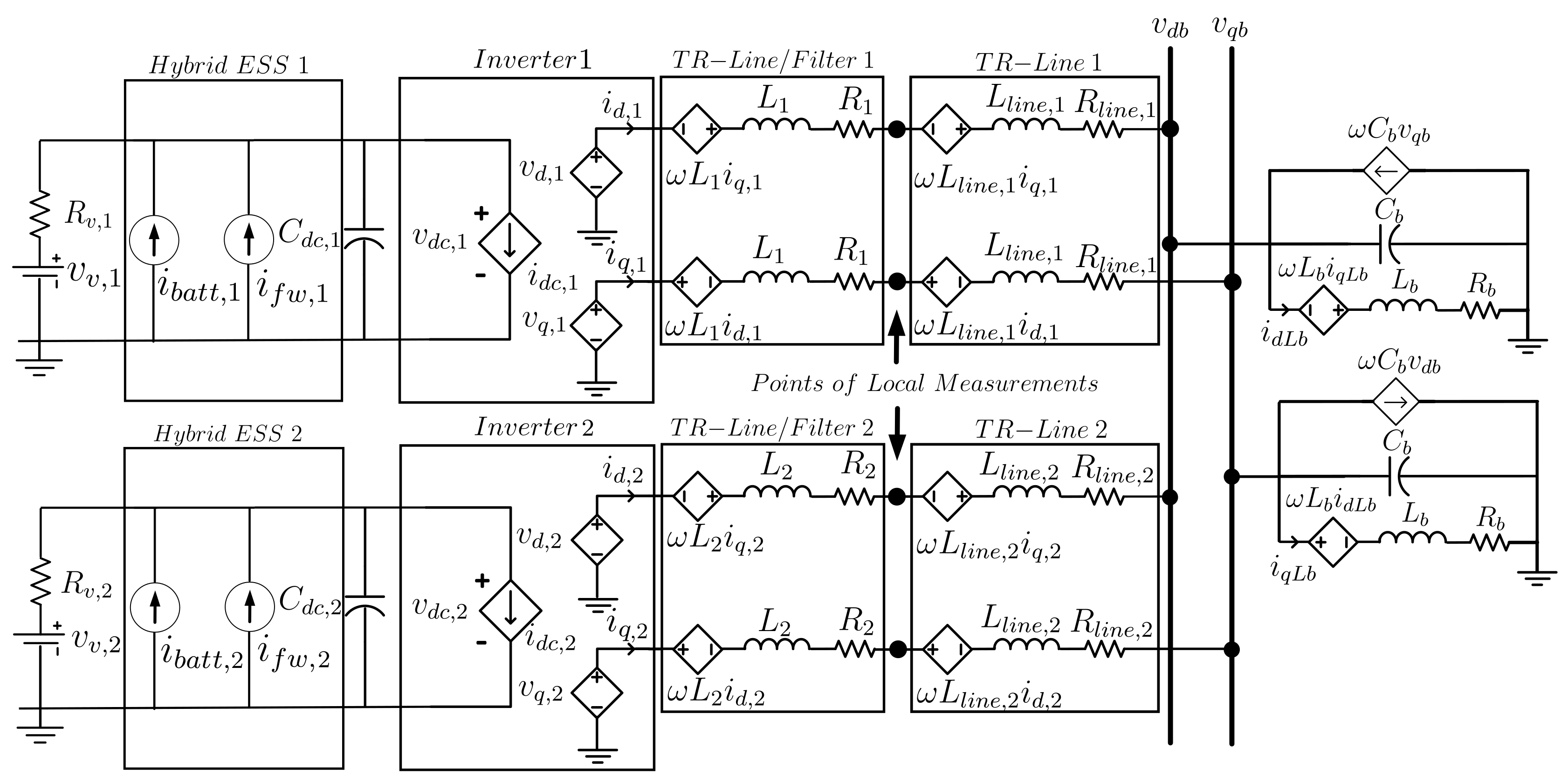
The overall system in Figure 2 with parameters in

Table 1. Microgrid Parameters.

DGU Parameters
ine	$L\left(\mu H\right)$	$R(\Omega )$	$C_{dc}\left(\mu F\right)$	$R_v(\Omega )$
ine DGU 1	1	0.2	100	0.5
ine DGU 2	2	0.25	150	0.5
Line Parameters
ine	$R_{line}(\Omega )$		$L_{line}\left(\mu H\right)$
ine $T{R}_{line,1}$	0.1		20
ine $T{R}_{line,2}$	0.15		10
Load Parameters
ine	$R_b(\Omega )$		$L_b\left(mH\right)$	$C_b\left(\mu F\right)$
ine Load	2		3	47

is simulated in Wolfram Mathematica, SystemModeler [27] and Modelica [28]. The system includes two DGUs that are connected to a common bus and an RLC load through $RL$ transmission lines. Two examples are presented in this section. For both cases, the ESSs aim to compensate for source fluctuations by enforcing the references that are fed by the local Hamiltonian control system. The arbitrary nominal value for the bus voltage is $240V_{pk-pk}$ and the secondary control scheme is defined so that the bus voltage always returns to this nominal value. This is a hard constraint for the operation of the system causes the overall MG system mimic a constant power load from source-side perspective. The aim is to maintain the bus voltage and the load power using the sources and the ESSs. It is assumed that the average power value of the source is sufficient to maintain the load and the ESS is utilized only to smooth the power to the average value. For the load voltage of $240V_{pk-pk}$, the corresponding nominal d-q voltages $V_{db}^{*}$ and $V_{qb}^{*}$, are $147V$ and $0V$ respectively. Voltage sources $v_{v,1}$ and $v_{v,2}$ have randomly chosen dc values around $300V$ with superimposed uniform random white noise with amplitude of less than $20V_{pk-pk}$. A practical constraint to consider is that the source voltages cannot have values less than the corresponding dc bus voltages $v_{dc,1}$ and $v_{dc,2}$. The random voltage component aims to introduce fluctuations so that the contributions of ESSs with different bandwidths are presented for a worst-case scenario for a field deployed MG.

In the first example, load power is solely supported by one DGU and droop control is set so that DGU 2 does not contribute to the load power. This baseline example aims to demonstrate the efficacy of the combination of the Hamiltonian control in (25) and demonstrate the trade-off between the ESS response versus the electrical level regulation of the system. The results are shown in Figure 3, Figure 4, Figure 5, Figure 6, Figure 7, Figure 8, Figure 9, Figure 10, Figure 11, Figure 12 and Figure 13 for a single ESS element with first-order model in (33a). In the second example, the system in Figure 2, under primary droop control in (26), secondary control in (31) and Hamiltonian control in (25) is simulated. In this example, the steps in Section 8 are followed for load and source profiles shown in Figure 14. Step 5 however, is re-iterated to utilize the matched BESS and FESS models in Reference [11]; hence, the PI gains of the cascaded BESS controller in Reference [11] are optimized according to (50) to match the first-order LPF.

It is important to note that the aim of ESS sizing in these examples is not to determine BESS or FESS device component parameters. Instead, the intent is to analyze the power split using the sizing criteria in (40) and observe the subsequent energy allocation. Hence, the power and energy sizing are done from the perspective of the Point of Common Coupling (PCC) between the DC-link and individual BESS and FESS subsystems. Sizing an energy storage device for its specific components and parameters under various DLCs and Energy Management Systems (EMSs) requires device-specific design measures, rigorous analysis and addressing multiple trade-offs at device and control levels which are out of the capacity of this work. Hence, the simulation cases are designed to serve the objective of the proposed control rather than to dictate detailed device-specific component sizing.

9.1. Single DGU with Constant Load Example

A $6s$ simulation of the system is performed for a fixed load value of $R_b=2\Omega$. The source voltage with superimposed sampled variable voltage is shown in Figure 3. The results for a band-limited ES element with cut-off frequency of ${\omega }_{cut-off}=1000\mathrm{rad}/\mathrm{s}$ are presented in Figure 4, Figure 5, Figure 6, Figure 7 and Figure 8. The maintained three-phase bus voltages and the injected load currents are shown in Figure 4a,b respectively. Figure 5 shows the dc bus voltage and Figure 6 demonstrates the current of the band-limited ES element. Figure 7a,b demonstrate the bus voltage and injected load current amplitude fluctuations respectively. Direct and quadrature current components, $i_d$ and $i_q$, represent the injected current to the bus/load and are shown in Figure 7c,d.

The overall dc power of the source and the ESS is presented in Figure 8a. Figure 8b shows dc power is delivered to the load with some reduction due to the transmission line losses. The significant loss is expected since the system is under load of $2\Omega$ at $240V_{pk-pk}$ bus voltage. The contributing ESS dc power is demonstrated in in Figure 8c.

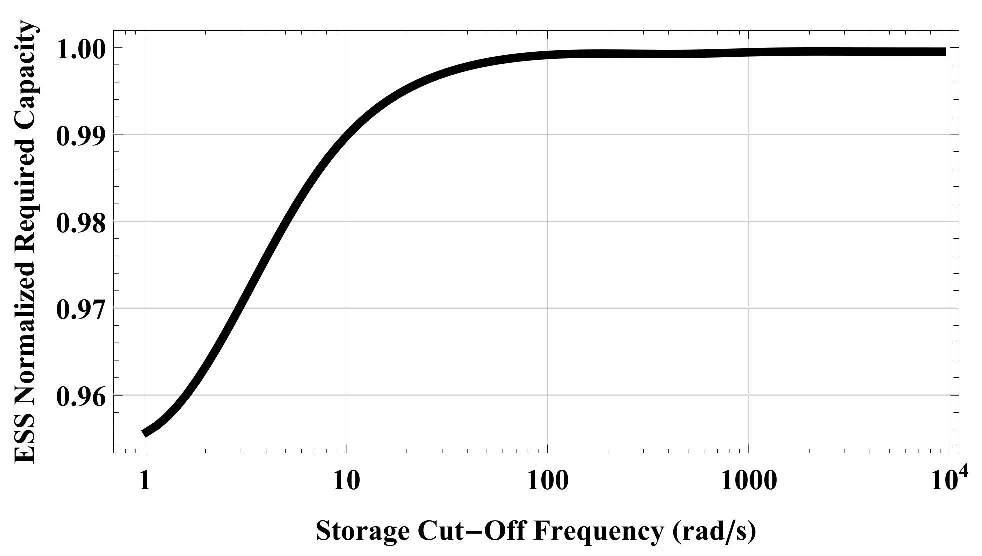
Figure 9, Figure 10 and Figure 11 represent the dc bus voltage when the ESS cutoff frequency ${\omega }_{cut-off}$ is $10\mathrm{rad}/\mathrm{s}$, $100\mathrm{rad}/\mathrm{s}$ and $10000\mathrm{rad}/\mathrm{s}$ respectively. The overall sweep of the ESS cut-off frequency versus dc voltage quality is demonstrated in Figure 12. It can be seen that there is a trade-off between the ESS size and bandwidth of operation and the voltage fluctuations in dc bus. Figure 13 demonstrates the required normalized capacity against the bandwidth sweep. The normalized capacity is obtained by dividing the required capacity at specific frequency support over the maximum required capacity when an ideal ES element is present. It is important to understand that in this example, the aim is to put the most possible stress on the ESS. Typically, filters such as dc reservoir capacitors are chosen significantly larger than the ones chosen for system in Figure 2. Bus fluctuations that have higher frequency contents can generally be attenuated with such capacitors, however, here such capacitors are down-sized to highlight the behaviour of the control.

9.2. Parallel DGUs Example

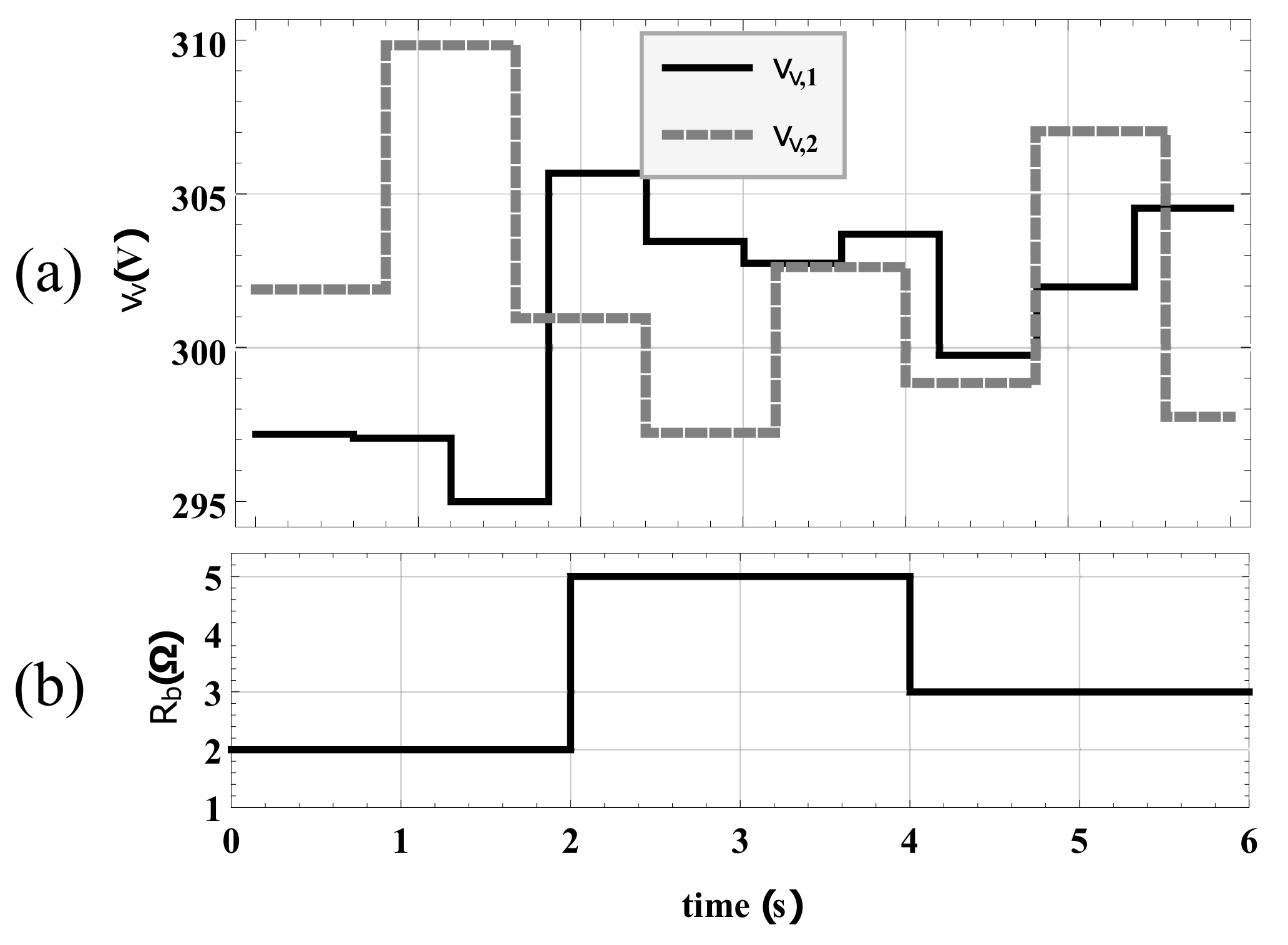
In this example, the two DGU system in Figure 2 with parameters in Table 1 and under droop control with weighting of 1:2 is considered. The source and load profiles are shown in Figure 14. Considering the guidelines in Section 8, first, the system is run with an ideal ESS model. The corresponding reference powers, $P_{ESS,1}$ and $P_{ESS,2}$ are shown in Figure 15. From (43), the overall required energy capacities, for $DG{U}_1$ and $DG{U}_2$ are $5159.9J$ and $4529.9J$ respectively. For BESS power-share of more than $95\%$, the overall RMS of the power signals are obtained as $2042RMS$ and $2408RMS$ for $DG{U}_1$ and $DG{U}_2$ respectively. Moreover, according to (39), with $\gamma =95\%$, the cut-off frequencies are found to be $12.56\mathrm{rad}/\mathrm{s}$ and $18.84\mathrm{rad}/\mathrm{s}$ for filters corresponding to $BES{S}_1$ and $BES{S}_2$. With the individual cut-off frequencies known, the control gains of BESSs from Reference [11] are optimized to match first-order LPFs as shown in Figure 16 and Figure 17. The obtained gain values are shown in

Table 2. ESSs Parameters.

BESS Parameters			FESS Parameters
	$BES{S}_1$	$BES{S}_2$		$FES{S}_1$	$FES{S}_2$
ine $C_1\left(\mathrm{F}\right)$	750	640	$J_f\left({\mathrm{Kgm}}^2\right)$	0.91	0.95
$C_2\left(\mathrm{F}\right)$	400	300	$k_t\left(\mathrm{Nm}/\mathrm{A}\right)$	1	1
$C_u\left(\mathrm{uF}\right)$	10	20	$R_{pm}(\mathrm{m}\Omega )$	47	54
$L_1\left(\mathrm{uH}\right)$	17	19	$L_{pm}\left(\mathrm{mH}\right)$	14	11
$L_u\left(\mathrm{mH}\right)$	20	25	$C_u\left(\mathrm{mF}\right)$	2	1.7
$R_1(\mathrm{m}\Omega )$	0.1	0.14	$R_{cu}(\mathrm{K}\Omega )$	1	1
$R_{c,1}(\mathrm{K}\Omega )$	10	10	$L_u\left(\mathrm{mH}\right)$	20	14
$R_{c,2}(\mathrm{m}\Omega )$	0.24	0.3	$R_u(\mathrm{m}\Omega )$	120	109
$R_{cu}(\Omega )$	100	110	$B(\mathrm{Nm}/{\displaystyle \frac{\mathrm{rad}}{\mathrm{s}}})$	0.001	0.0019
$R_{Lu}\left(\mathrm{mH}\right)$	100	150	$N_{s,fw}$	1	1
$V_{oc}\left(\mathrm{V}\right)$	48	48	$N_{p,fw}$	1	1
$Q\left(\mathrm{Ah}\right)$	10	15	$k_i$	10	10
$N_{s,batt}$	2	2	$k_p$	1	1
$N_{p,batt}$	4	5
$k_{i,u}$	3.03	7.79
$k_{p,u}$	0.64	1.36
$k_{i,batt}$	120	106
$k_{p,batt}$	3.73	2.92

.

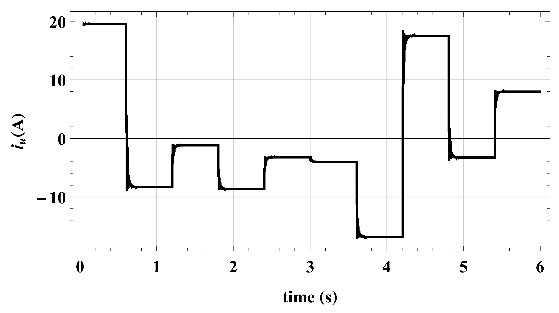
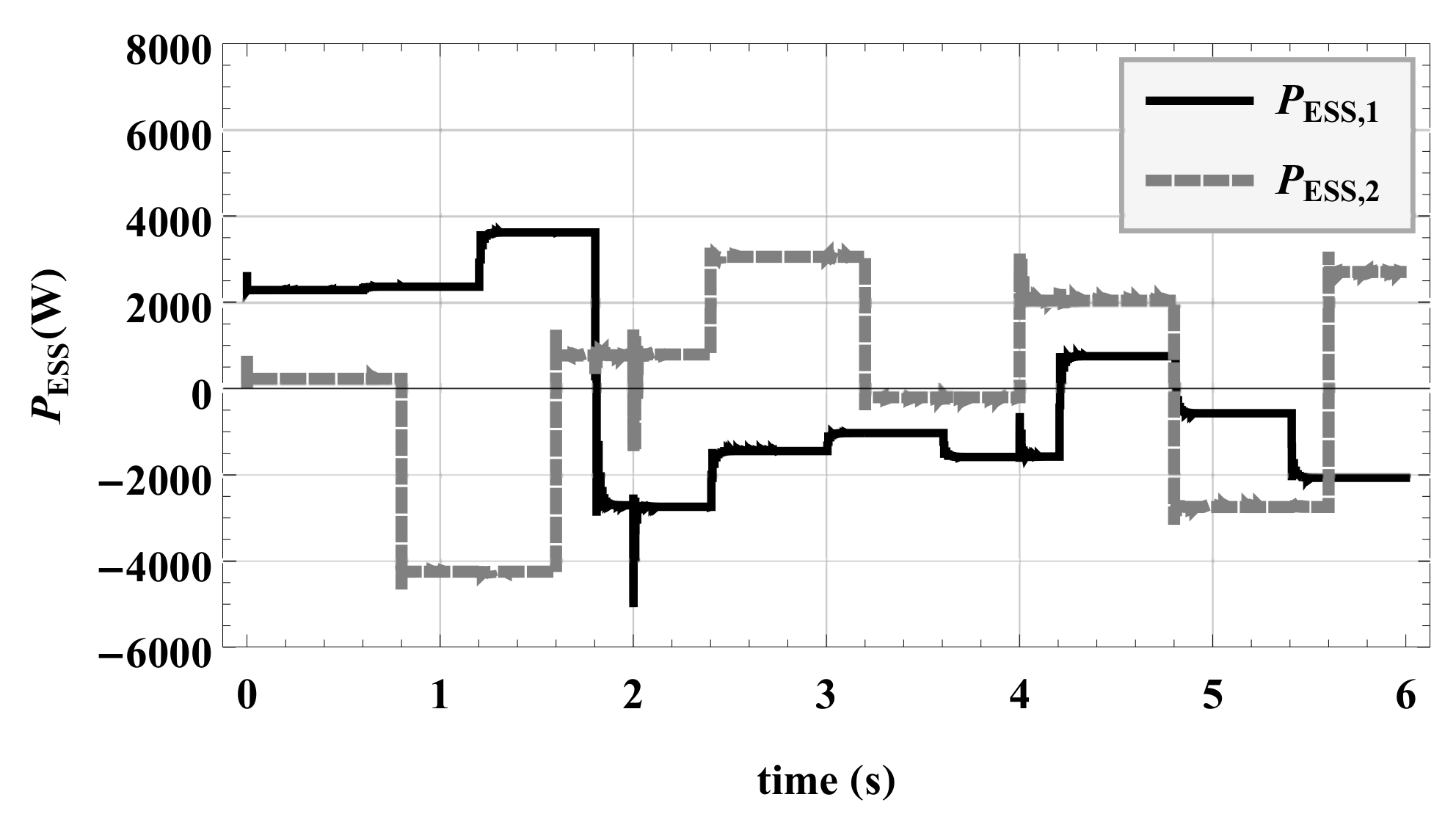
The simulation is re-run and the BESS with specified control gains are used. The system performance is shown in Figure 18, Figure 19, Figure 20, Figure 21 and Figure 22. Figure 18 demonstrates individual hybrid current contributions for BESSs and FESSs. It can be seen that significant low-frequency portions of the currents are allocated to BESSs, and the FESSs are requested only for high power and fast fluctuations. As mentioned before, for energy density sizing, the overall injected power (or current) from the ESS device is considered rather than detailed specification of battery and flywheel system components. The obtained BESS RMS contributions are $1957.3RMS$ and $2306.6RMS$ corresponding to $95.84\%$ and $95.78\%$ of the total RMS of the power signals. Using (41) and (43), the total required energy from $BES{S}_1$ and $BES{S}_2$ are $4836.1J$ and $4372.7J$ respectively which match the expected results with an acceptable accuracy. 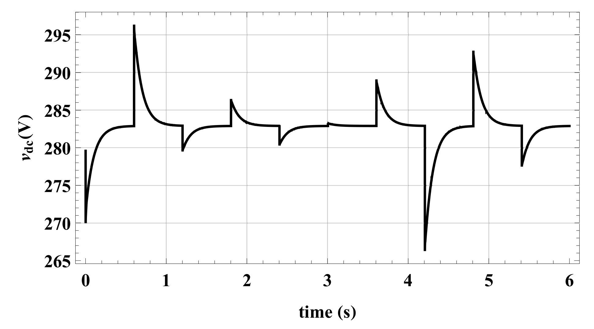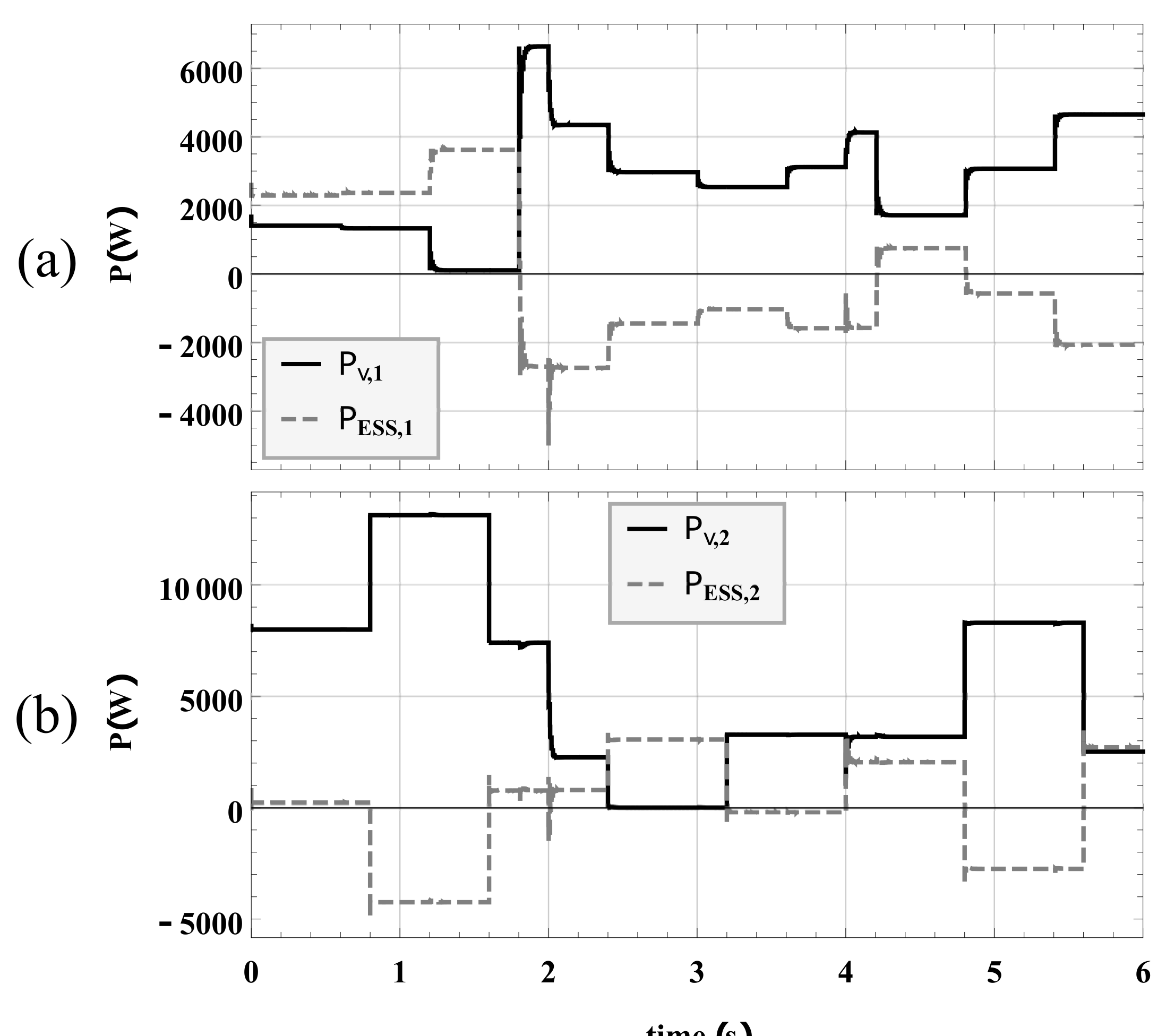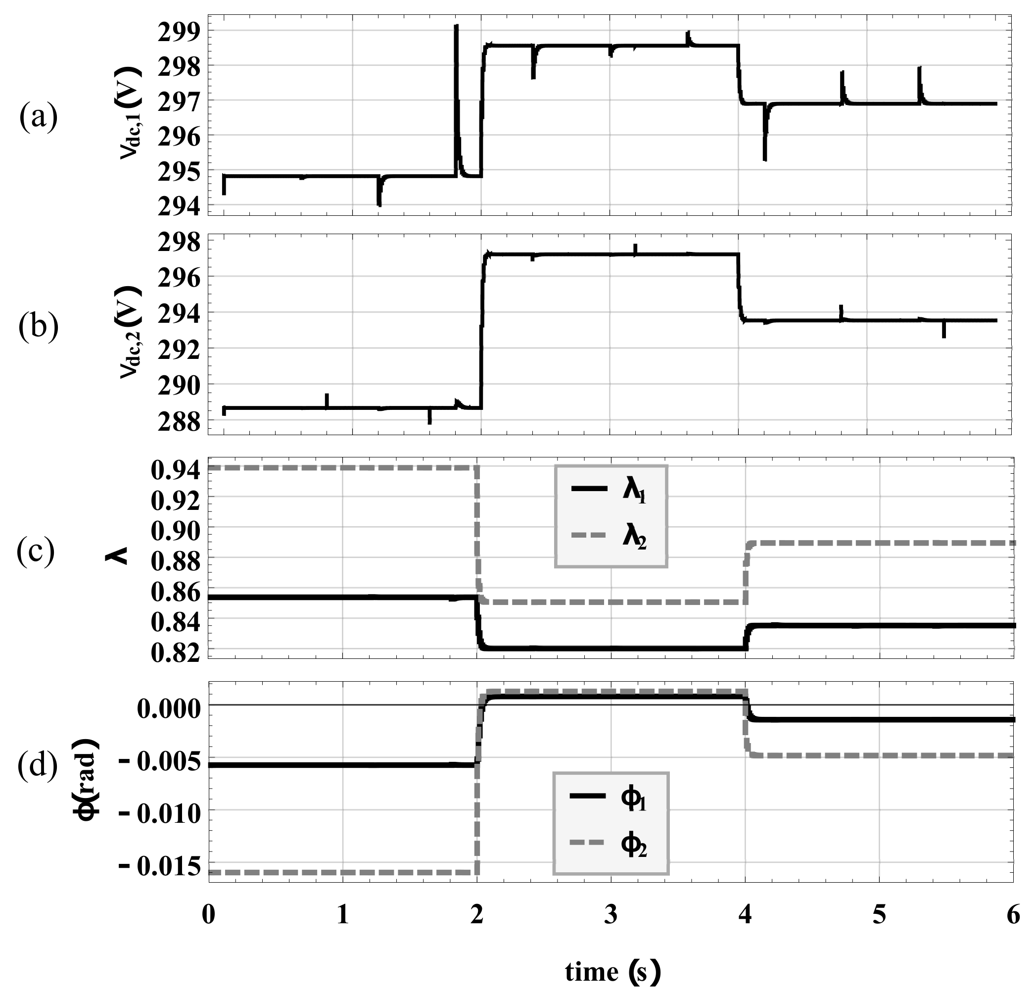Figure 19 presents the source powers and overall ESSs dc powers. Individual dc-link voltages, $v_{dc,1}$ and $v_{dc,2}$ are shown in Figure 20a,b respectively. It can be seen that ESSs regulate dc voltages versus the source fluctuations rather than the load which is consistent with the results of the previous example. However, in constant load periods, $v_{dc}$ variations are relatively smaller which demonstrate the efficacy of the hybrid ESSs for power bandwidth support. Figure 20c,d demonstrate the dynamics of individual inverter commands $(\lambda ,\varphi )$ for the two DGUs.

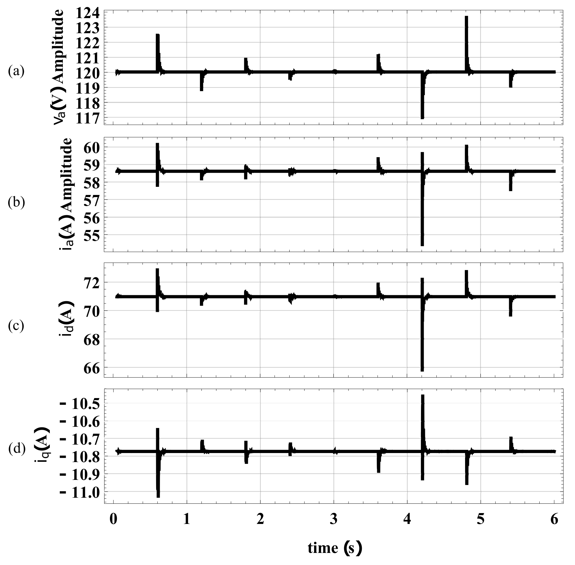
Considering the load-side bus, Figure 21 shows real and reactive power sharing under the droop control. ${\gamma }_1$ and ${\gamma }_2$ from (28) are chosen to be $0.33$ and $0.66$ respectively. It can be seen that the power sharing is effectively maintained versus the load changes. The maintained three-phase bus voltage is demonstrated in Figure 22a. It is evident that as the sources and load fluctuate, the three-phase ac bus amplitude (denoted by phase a voltage $v_a$) is kept at $240V_{pk-pk}$. Figure 22b shows the corresponding load current while Figure 22c demonstrates the shared three-phase currents which both are consistent with the specified 1:2 power sharing weightings.

10. Conclusions and Future Work

In this paper, the HSSPFC method derivations, under hierarchical control and for parallel topology of source and ESS were presented. Specific constraints were defined and added to the control law to put the parallel ESS at zero output conditions and compensate for source-side fluctuations. A simple power splitting method for hierarchical ESS control was defined and utilized to size hybrid BESSs and FESSs for the corresponding power densities. The results attest if the LPF and the band-limited BESS frequency responses are matched, the described power sharing based on power spectrum yields accurate results. The performance of a MG system with hybrid ESSs and two DGUs under d-q droop control versus variable sources and load was demonstrated.

Most of the assumptions in this article can be challenged for future work. The control law defined in (25) will further be modified to account for constraints that address various control scenarios such as power smoothing [13], MPPT [15], peak shaving [14] and power curtailment [12]. Moreover, detailed device controllers such as in Reference [29] will be used to specify and integrate series battery module control. Furthermore, design of more detailed Power Management Systems (PMSs) based on Wavelet transform methods [30] can also be investigated.