A Low Complexity, High Throughput DoA Estimation Chip Design for Adaptive Beamforming

Abstract

Direction of Arrival (DoA) estimation is essential to adaptive beamforming widely used in many radar and wireless communication systems. Although many estimation algorithms have been investigated, most of them focus on the performance enhancement aspect but overlook the computing complexity or the hardware implementation issues. In this paper, a low-complexity yet effective DoA estimation algorithm and the corresponding hardware accelerator chip design are presented. The proposed algorithm features a combination of signal sub-space projection and parallel matching pursuit techniques, i.e., applying signal projection first before performing matching pursuit from a codebook. This measure helps minimize the interference from noise sub-space and makes the matching process free of extra orthogonalization computations. The computing complexity can thus be reduced significantly. In addition, estimations of all signal sources can be performed in parallel without going through a successive update process. To facilitate an efficient hardware implementation, the computing scheme of the estimation algorithm is also optimized. The most critical part of the algorithm, i.e., calculating the projection matrix, is largely simplified and neatly accomplished by using QR decomposition. In addition, the proposed scheme supports parallel matches of all signal sources from a beamforming codebook to improve the processing throughput. The algorithm complexity analysis shows that the proposed scheme outperforms other well-known estimation algorithms significantly under various system configurations. The performance simulation results further reveal that, subject to a beamforming codebook with a 5° angular resolution, the Root Mean Square (RMS) error of angle estimations is only 0.76° when Signal to Noise Ratio (SNR) = 20 dB. The estimation accuracy outpaces other matching pursuit based approaches and is close to that of the classic Estimation of Signal Parameters Via Rotational Invariance Techniques (ESPRIT) scheme but requires only one fifth of its computing complexity. In developing the hardware accelerator design, pipelined Coordinate Rotation Digital Computer (CORDIC) processors consisting of simple adders and shifters are employed to implement the basic trigonometric operations needed in QR decomposition. A systolic array architecture is developed as the computing kernel for QR decomposition. Other computing modules are also realized using various linear systolic arrays and chained together seamlessly to maximize the computing throughput. A Taiwan Semiconductor Manufacturing Company (TSMC) 40 nm CMOS process was chosen as the implementation technology. The gate count of the chip design is 454.4k, featuring a core size of 0.76 ${\mathrm{mm}}^2$, and can operate up to 333 MHz. This suggests that one DoA estimation, with up to three signal sources, can be performed every 2.38 μs.

1. Introduction

Beamforming is a technique of transmitting signal to or receiving signal from a designated direction. Because of the discrepancy in treating signals from different directions, it is also known as filtering in the space domain. Beamforming has been widely used in radar, wireless communication and medical imagining systems and requires an antenna (or transducer) array to accomplish it. By properly controlling the phases and amplitudes of signal on each antenna, the transmission or reception signal gain along specific directions can be enhanced while those along other directions will be suppressed. The benefits of beamforming include improved link budget, extended service range and interference suppression. In adaptive beamforming, the beams are not fixed. Instead, they are steered dynamically toward the directions of signal sources. Although not all beamforming applications require explicit directional information of the signal sources, DoA estimation is essential in radar signal processing and establishing wireless communication links. Explicit DoA information also helps achieve better interference cancellation.

1.1. Related Works of DoA Estimation

The basics of DoA estimation is exploring the phase differences of signals received from an antenna array to distinguish the signal direction. In the presence of multiple signal sources and background noises, the orthogonal property between the noise and signal subspaces is assumed. The first step of estimation is calculating the auto-correlation matrix using the received antenna array signals. A uniformly spaced (by a pitch of ½ ) linear antenna array is assumed for 1-D (azimuth angle) estimation. The Radio Frequency (RF) signals are down converted to baseband and form a signal vector x(t) in each digital sampling. If the RF modulation does include both in-phase and quadrature phase components, an additional Hilbert transform is needed to obtain complex-valued signal vectors. Conventional estimation schemes can be classified into three categories, i.e., noise subspace, signal sub-space and matching pursuit. For the noise subspace approach, the noise subspace is determined using the auto-correlation matrix. A MUSIC (MUltiple SIgnal Classification) scheme and its variations [1,2,3] perform Eigenvalue Decomposition (EVD) to obtain the noise sub-space spanned by the Eigen vectors corresponding to smaller Eigen values. The Eigen vectors of noise sub-space are used to construct a spatial frequency spectrum function. A spatial frequency scanning procedure is next performed and the peaks of the spectrum indicate the directions of signal sources. In [4,5], a ROOT-MUSIC scheme, aimed at eliminating the expensive spatial frequency scanning procedure by finding the roots of a nonlinear polynomial, was proposed. In [6], the noise space estimation is improved by applying oblique projection along the signal sub-space.

For the signal sub-space approach, on the contrary, the signal sub-space is extracted via auto-correlation matrix decomposition. Instead of spectrum scanning, the signal directions are computed directly. ESPRIT (Estimation of Signal Parameters Via Rotational Invariance Techniques) [7,8,9] is considered a classic scheme of this category. It applies the singular value decomposition first and uses the left singular matrix to represent the signal sub-space. By finding the transform matrix between the two sub-matrices of the singular matrix, all signal directions can be determined simultaneously following an additional Eigen value decomposition. Enhanced schemes such as [10] employs an additional time-frequency data model exhibiting multi-invariance to improve the estimation accuracy and scheme [11] can tackle the coherent signal detection problem. These two categories of estimation are computationally intensive because of various matrix decompositions, which requires iterative computations to obtain the results.

The third category of estimation scheme assumes a codebook (or dictionary matrix) consisting of steering vectors is available. A steering vector outlines the phase differences of received signals of the antenna array subject to a specific direction of arrival. The estimation is performed by finding the best match from the codebook using some greedy schemes such as Matching Pursuit (MP) [12,13,14]. The size of the codebook indicates the angular resolution of the estimation. Since the codebook is not orthogonal (steering vectors are not mutually orthogonal), the accuracy of matching can be degraded if the angular separation of two signal sources is small. In view of this, an enhancement using Orthogonal Matching Pursuit (OMP) [15], which calls for an extra orthogonalization process after each match, was proposed. Other improvements include the scheme in [16], which introduces an extra majorization–minimization measure, and the scheme in [17], which applies a conjugate gradient method with subtraction method. In [18], the performance of the OMP scheme is enhanced with iterative local searching. In [19], the OMP scheme is applied to hybrid non-uniform array. Although this category of estimation schemes is considered less computation demanding than the first two counterparts, expensive computations such as pseudo matrix inverse computations are still needed.

1.2. Motivations and Contributions

Note that the frequency of performing DoA estimation in adaptive beamforming can be high, in particular, in fast time varying environments such as for vehicular communications. In addition, array signal processing is computationally intensive and the algorithms usually exhibit a complexity of O(N³), where N is the antenna array size. For radar systems employing hundreds of antenna, the computing requirement is humongous. Therefore, conventional programmable digital signal processor approaches may not be able to process the data in real time and only the hardwired approaches are feasible. Hardwired approaches also provide much better power consumption than programmable approaches. To achieve an efficient hardware accelerator design, we need to 1) reduce the computing complexity of the algorithm, and 2) map the algorithm neatly to a hardware architecture supporting massive parallel processing and pipelined operations. In this paper, we aim at tackling these two issues and develop a low complexity, high throughput, DoA estimation accelerator design in chip.

The contributions of this work can be summarized as follow: In the algorithm development perspective, various design measures were devised to facilitate low complexity DoA estimations. These include applying a signal sub-space projection to enhance the accuracy of matching pursuit, calculating only a subset of auto-correlation matrix to avoid computing redundancy, and simplifying the projection matrix computation via QR factorization, which factorizes a matrix to the product of a unitary matrix Q and an upper triangular matrix R. These measures successfully reduce the computing complexity to only one fifth that of the ESPRIT scheme while largely maintaining the estimation accuracy. In the hardware accelerator design perspective, an effective algorithm to hardware mapping was conducted. Efficient systolic array designs were developed for each computing module and integrated seamlessly to avoid any data disruption between modules. The data input scheme was taken into consideration when determining data buffering and hardware allocation. This avoids excessive computing concurrency and minimizes the hardware complexity. An efficient QR factorization design based on the Coordinate Rotation Digital Computer (CORDIC) units was also developed. All of these design measures and innovations can be equally applied to likewise designs. Finally, a chip design in TSMC 40 nm CMOS process technology was presented to demonstrate the significant speed up can be achieved. The gate count of the chip design is 454.4 k and can operate up to 333 MHz. This suggests that one DoA estimation, with up to three signal sources, can be performed every 2.38 μs.

The rest of the paper is organized as follows: in Section 2, a brief recap of three DoA estimation schemes, i.e., ESPRIT, Matching Pursuit (MP) and Orthogonal Matching Pursuit (OMP), used in the performance comparison is given first. The proposed projection based parallel matching pursuit (P²MP) scheme is next presented. In Section 3, the performance evaluations of the proposed scheme against existing ones are described. The evaluations include computing complexity, estimation accuracy and how DoA estimation enhances Frequency Modulated Continuous Waveform (FMCW) radar detection. The performance robustness of the proposed scheme to the assumption of the number of signal sources is also verified. In Section 4, the target application of the proposed DoA estimation scheme and the hardware design specifications are first introduced. The system architecture, timing diagram, and individual hardware module designs are next elaborated followed by a chip implementation report and comparison with existing works.

2. Projection and Parallel Matching Pursuit Based DoA Estimation

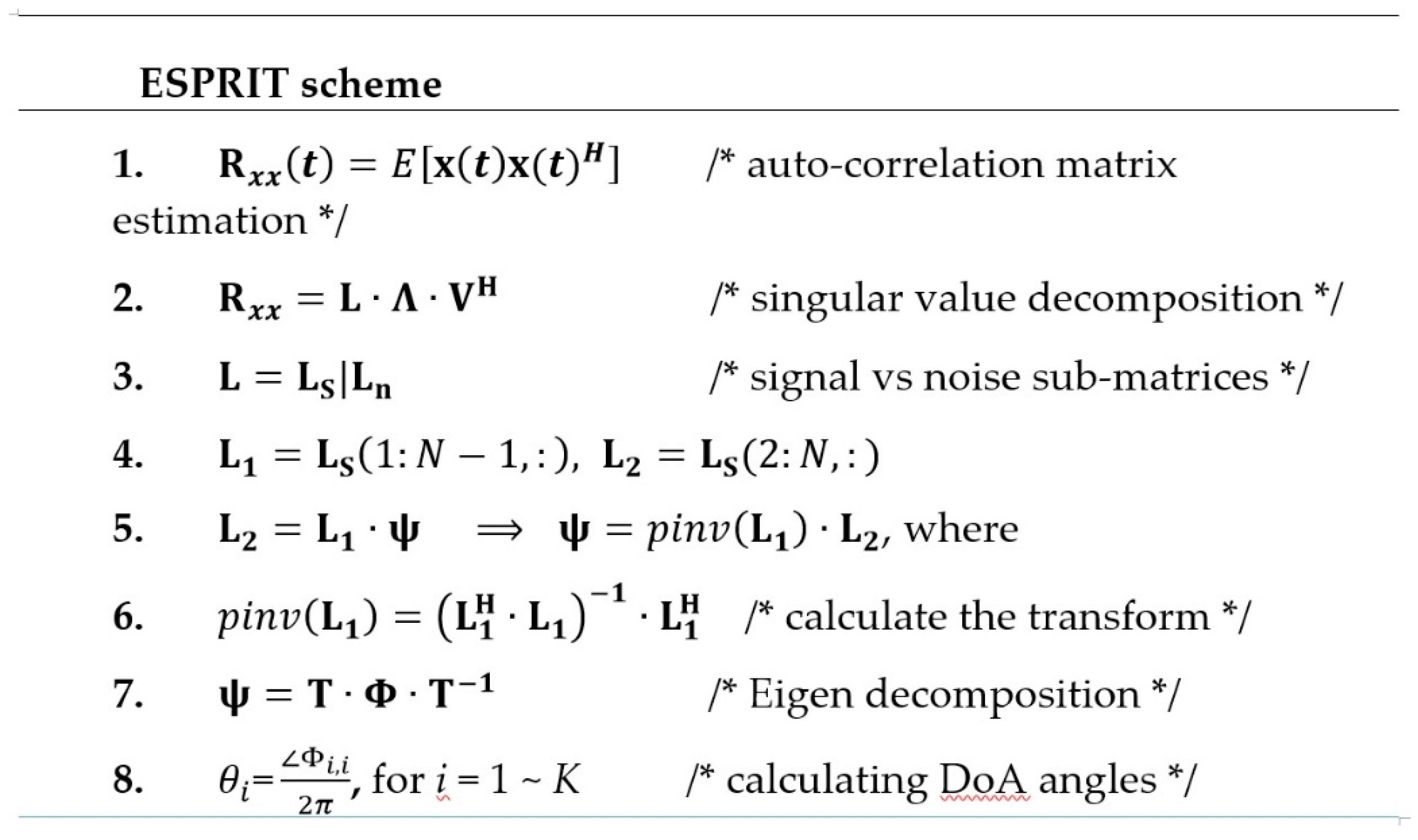
2.1. Recap of Conventional DoA Estimation Schemes

Before introducing the proposed DoA estimation schemes, three popular schemes are reviewed first to highlight computing complexity issue and the difference with the proposed one. The first one is the ESPRIT scheme [7,8,9], which is a classic signal sub-space based approach. The corresponding pseudo code is shown in Figure 1. An auto-correlation matrix is estimated first followed by a singular matrix decomposition. The number of signal sources can be determined by counting the number of significant singular values. The column vectors of the left singular matrix corresponding to those significant singular values form a sub-matrix $L_S$, which spans the signal sub-space. $L_S$ is further divided into two sub-matrices $L_1$ and $L_2$ by taking the N-1 and the last N-1 rows, respectively. This means each matrix is derived using signals from N-1 out of N antennas. There thus exists a transform $\mathsf{\psi }$ between $L_1$ and $L_2$. The transform matrix $\mathsf{\psi }$ can be calculated by taking the pseudo matrix inversion. Finally, the Eigen decomposition of $\mathsf{\psi }$ is performed and the angular information of Eigen values indicate the directions of arrival. The advantage of this approach is that no prior information of the number of signal sources is needed. In addition, all signal sources can be identified simultaneously. The obvious shortcoming of this scheme is its computing complexity. Both singular value and Eigen decompositions are computationally intensive and can only be solved through iterative procedures and the computing complexity of each iteration is of order O(N³) [20]. The pseudo inverse calculation, which requires two matrix multiplications and one matrix inversion, also bears a complexity of O(N³). These computing requirements become a big hurdle to high throughput rate in implementation.

In contrast to calculating the angles of DoA directly, the matching pursuit based approaches [12,13,14] try to identify them from a codebook with a pre-defined angular resolution. Unlike the ESPRIT scheme, they are free of expensive matrix decompositions and inversions. Instead, a sparse approximation algorithm, which finds the "best matching" projections of multidimensional data onto the span of an over-complete dictionary matrix, is conducted. Best matching means a minimum number of vectors in the dictionary matrix are selected. The selection or matching process is in general greedy and conducted progressively. The original MP scheme works well in the presence of only one signal source but the performance degrades as the number of signal sources increase. Therefore, the enhanced scheme OMP [15] was presented. Figure 2 shows a combined pseudo code of the MP/OMP schemes. The residual matrix R is initially set to the auto-correlation matrix $R_{xx}$. Assume there are K signal sources, they are identified one by one using a for loop. In each loop iteration, the residual matrix is multiplied with the codebook matrix D, and the vector (in the codebook) yields the maximum norm 2 value after multiplication is considered the “best match”. The corresponding index p is added to the set P. For OMP, an additional step 8 is performed, i.e., the matched vector is appended to a matrix A. After the vector selection, in the MP scheme, the contribution of the selected vector is subtracted from the residual matrix (step 9). In the OMP scheme, an orthogonalization process (step 10) is performed. It uses all the selected vectors instead of the current one to calculate the residual matrix R. In other words, the projection of residual matrix R on the vector space spanned by all the selected vectors is removed. This calls for a pseudo matrix inversion, pinv(A), defined as:

$$pinv\left(A\right)={(A^H·A)}^{-1}·A^H$$

(1)

where the superscript H indicates taking the complex-conjugate and transpose of the matrix. This is the major distinction between the original MP scheme and the orthogonal MP scheme. In addition, the residual matrix is recalculated in each loop iteration while that of the MP scheme is updated incrementally. The orthogonalization process facilitates better matching result in subsequent vector selection [15]. The computing complexity, however, increases significantly. The matching process proceeds until either the matrix norm of the residual matrix is smaller than a threshold $\mathbf{\epsilon }$ or the loop iteration ends. It should also be noted that the matching processes in both schemes are basically sequential and cannot be processed in parallel. In summary of this recap, the MP and the OMP schemes, in spite of a limited angular resolution in estimation confined by the codebook size, does exhibit a significant advantage in computing complexity over the ESPRIT scheme. The orthogonalization process employed in the OMP scheme helps improve the estimation performance in the presence of multiple signal sources, but, in the meantime, negatively impacts the computing complexity.

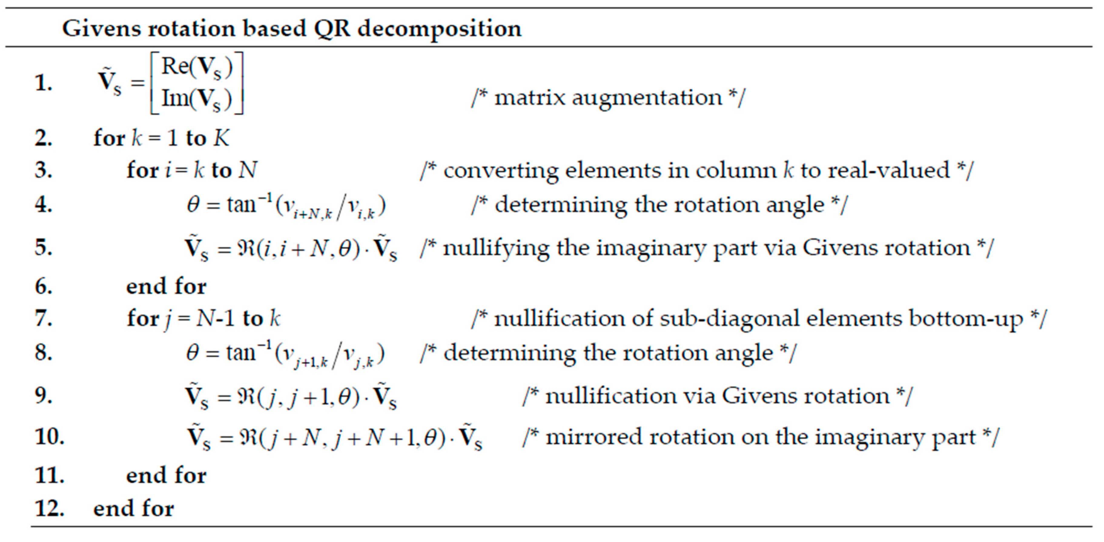
2.2. Proposed DoA Estimation Algorithm

In view of the concerns discussed earlier, a new scheme, called Projection and Parallel Matching Pursuit (P²MP) is proposed. Our idea is combining the merits of sub-space and codebook search approaches, i.e., applying signal projection first before performing matching pursuit. In other words, the matching pursuit is performed in the signal sub-space. This measure helps minimize the interference from noise sub-space and makes the matching process free of extra orthogonalization computations. The computing complexity can thus be reduced significantly. In addition, estimations of all signal sources can be performed in parallel without going through a successive update process. Further optimization measure is employed to alleviate the computing efforts of signal projection. Instead of using expensive pseudo matrix inversion, the projection matrix calculation is accomplished by applying a partial QR factorization to the auto-correlation matrix. Figure 3 shows the proposed P²MP DoA estimation scheme.

Assume there are K signal sources, the degree of signal sub-space is thus K. Therefore, we may choose the first (or arbitrary) K columns from $R_{xx}$ to form a sub-matrix $V_S$, which is supposed to span the signal sub-space. Given a codebook matrix $D_{N\times M}$ consisting of M dimension-N steering vectors, each of them is projected to the signal sub-space first. To accomplish this, a projection matrix corresponding to $V_S$ is calculated. Equation (2) show the expression of a projection matrix, which is equal to multiplying $V_S$ with its pseudo inverse matrix pinv($V_S$).

$$P_S=V_S·{\left(V_S{}^t·V_S\right)}^{-1}·V_S{}^t$$

(2)

A straightforward computing scheme would require 3 complex-valued matrix multiplications and one matrix inversion. To alleviate the computing demand, a QR decomposition is applied to $V_S$ first.

$$V_S=Q_{S,N\times K}·R_{K\times K}$$

(3)

where $Q_{S,N\times K}$ is a unitary matrix consisting of K orthonormal vectors and $R_{K\times K}$ is an upper triangular matrix. The choice of QR decomposition is that it can be efficiently supported in hardware implementation. This will be elaborated later in Section 3. The calculation of projection matrix $P_S$ is then simplified subject to the decomposition result.

$$\begin{array}{ll}{P}_S& =V_S·{(V_S^H·V_S)}^{-1}·V_S^H\\ & =Q_{S}R·{(R^H{Q}_S^H·Q_{S}R)}^{-1}·R^H{Q}_S^H\\ & =Q_{S}R·R^{-1}{(R^H)}^{-1}·R^H{Q}_S^H=Q_S·Q_S^H\end{array}$$

(4)

Note that $Q_S^H·Q_S=I_{K\times K}$ due to its unitary property and $Q_S·Q_S^H$ yields an N by N projection matrix. The simplification result indicates the projection matrix can be obtained by a simple matrix multiplication. After obtaining the projection matrix, all vectors $\mathit{a}\left({\theta }_i\right)$ in the codebook are projected to the signal sub-space spanned by $V_S$ and those K vectors with largest norm 2 values after projection correspond to the DoA of K signal sources, respectively. Since all vector projections and the following norm 2 value comparisons can be performed in parallel (as indicated by the forall loop), this can greatly speed up the matching process while purely sequential processes are performed in the MP and OMP schemes.

The most complicated computing module of the proposed scheme is QR decomposition. There are various computing schemes [21,22,23,24] using either Householder Transforms (HT) or Modified Gram Schmidt (MGS). It is demonstrated in [25] that a Givens Rotation (GR) based approach is the most efficient one. A (real-valued) Givens rotation is a trigonometric operation that rotates a 2-D vector by an angle. If the vector is rotated to one of the two coordinate axes, the corresponding element of the vector becomes zero (or nullified). In QR decomposition, the upper triangular matrix R can be obtained by applying a sequence of Givens rotations to nullify all sub-diagonal elements. Givens rotation is unitary and the product of multiple Givens rotations is also unitary. If the matrix is complex-valued, complex-valued counterparts should be used. A complex-valued value Givens rotation can be realized by applying three real-valued Givens rotations as shown in Equations (5) and (6).

$$\left[\begin{array}{c}\left|\right|x\left|\right|\\ \left|\right|y\left|\right|\end{array}\right]=\left[\begin{array}{cc}{e}^{-j{\varphi }_1}& 0\\ 0& e^{-j{\varphi }_2}\end{array}\right]·\left[\begin{array}{c}x\\ y\end{array}\right]$$

(5)

$$\left[\begin{array}{c}r\\ 0\end{array}\right]=\left[\begin{array}{cc}\cos (\theta )& \sin (\theta )\\ -\sin (\theta )& \cos (\theta )\end{array}\right]·\left[\begin{array}{c}\left|\right|x\left|\right|\\ \left|\right|y\left|\right|\end{array}\right]$$

(6)

The first two convert complex-valued operands x, y respectively to their norm 2 values and the third one performs the nullification. Figure 4 shows the pseudo code of QR decomposition. The complex-valued $V_S$ is first made into a real-valued counterpart by stacking the real part on top of the imaginary part. The nullifications proceed from the first to the last (the K^th) column (the outer loop) and, in each column (the inner loops), proceed from the bottom to the top. This processing order prevents the occurrences of fill-in. Notation $\mathsf{\Re }(i,j,\theta )$ stands a real-valued Givens rotation operating on the i^th and the j^th rows of ${\tilde{V}}_S$ by an angle $\theta$. In implementation practices, the value of $\theta$ is not calculated explicitly. The details will be addressed when discussing the hardware implementation.

2.3. Computing Complexity Analysis

The performance evaluation of the proposed DoA estimation scheme against prior arts starts with the computing complexity analysis. Four DoA estimation schemes, the proposed P²MP, ESPRIT, MP and OMP, are compared. The results are summarized in

Table 1. Computing complexity analysis of different DoA estimation schemes.

Scheme	Complexity Formula
ESPIRIT	$21K^3+3K^2\left(N-1\right)+7K+21N^3$
MP	$\left(\left(M+1.5\right)N^2+\left(M+0.5\right)N\right)K$
OMP	$(N^3+\left(M+1\right)N^2+\left(M+2\right)N+1)K$
proposed	$2N^3+\left(M+K+1\right)N^2+\left(M-1\right)N$

. The measurement unit is a real-valued multiplication. Since we focus on the hardware implementation of DoA estimation schemes, the complexity of other type of computation is estimated as the ratio of its circuit complexity to that of a multiplier. The computing complexity of Givens rotation follows the estimation given in [14]. There are various iterative computing algorithms for singular value decomposition (SVD) and Eigen decomposition. The estimations are based on the numbers reported in [20]. The computing complexity of auto-correlation matrix estimation is excluded because it is common to all estimation schemes. Analytical forms of complexity formulae are derived for each scheme. Three parameters, i.e., N: the size of antenna array, K: the number of signal sources, and M: the size of codebook, are included. Table 1 shows the comparison results. The values subject to different combinations of (K, N, M) are illustrated in Figure 5.

Apparently, the ESPRIT scheme has the highest complexity because of the expensive SVD and ED computations. The number of antenna N is the dominant factor. The coefficient associated with the $N^3$ term is also the largest one because of the iterations in SVD and ED computation. The OMP scheme has the second highest complexity. Its complexity grows linearly with the number of signal sources, K, because of the orthogonalization process performed after every matching. The size of the codebook, M, also impacts the complexity in a linear way. The complexity of the MP scheme is lower than that of the OMP scheme by roughly 30%. The proposed P²MP scheme exhibits the lowest complexity in all but the (2,8,13) configuration. In that case, the MP scheme leads by a 3% margin. Although the number of signal sources, K, plays a role, it mainly affects the complexity of QR decomposition and its contribution to the overall complexity is less than direct proportionality. The complexity of QR decomposition is also independent of the codebook size, M. The complexities of MP/OMP schemes, however, grow linearly with the value of K. This explains the complexity advantage of the proposed scheme against the other three schemes. Note that the complexity of the proposed DoA scheme is independent of the Field of View (FoV). It is primarily affected by the codebook size. If angular resolution of steering vectors remains unchanged, then doubling the FoV would mean a twice large codebook. This will affect the parallel matching pursuit part but not the signal sub-space projection part. If the codebook size is fixed and a coarse angular resolution is adopted to cover a wider FoV, it will not affect scheme and the hardware design.

3. Simulation Results and Performance Analysis

3.1. Simulation Settings

For the performance analysis, we assume the antenna array size, N, is 8 and two codebook versions are adopted. The first one consists of 19 steering vectors (M = 19) uniformly spanning an FoV (Field of View) of 90°. The angular resolution is thus 5°. The second one has 10 steering vectors with an angular resolution equal to 10°. It should be noted that the half-power beam width for a sized N antenna array can be calculated as follows [26]:

$${\mathit{\theta }}_{3db}=50\frac{\lambda }{Nd}= \frac{100}{N} \left(deg\right),$$

(7)

where $d=\lambda /2$ is the inter-antenna element spacing. For N = 8, ${\mathit{\theta }}_{3db}$ is roughly 12.5°. For version 1 codebook, the angular resolution of the codebook is much finer than beam resolution and the overlap between two adjacent beams is high. This suggests a more challenging DoA estimation problem. For version 2 codebook, the angular resolution is similar to ${\mathit{\theta }}_{3db}$, which suggests a relaxed DoA estimation problem. The simulations are subject to four Signal to Noise Ratio (SNR) settings, i.e., 10, 20, 30 and 40 dB. The evaluation indexes are the percentage of incorrect estimates and the Root Mean Square (RMS) value of estimation error in incident angles based on the results of 100 simulation trials per case. The percentage is calculated on a per signal source basis. For the three codebook based schemes, an estimate error occurs if an incorrect vector is selected or a vector is chosen multiple times. For the ESPRIT scheme, an estimate error occurs if the estimated angle deviates from the correct one by half the codebook’s angular resolution. In each simulation trial, the directions of signal sources are randomly selected from the angles defined in the codebook. This is to exclude the factor of estimation error attributed to limited angular resolution of the codebook.

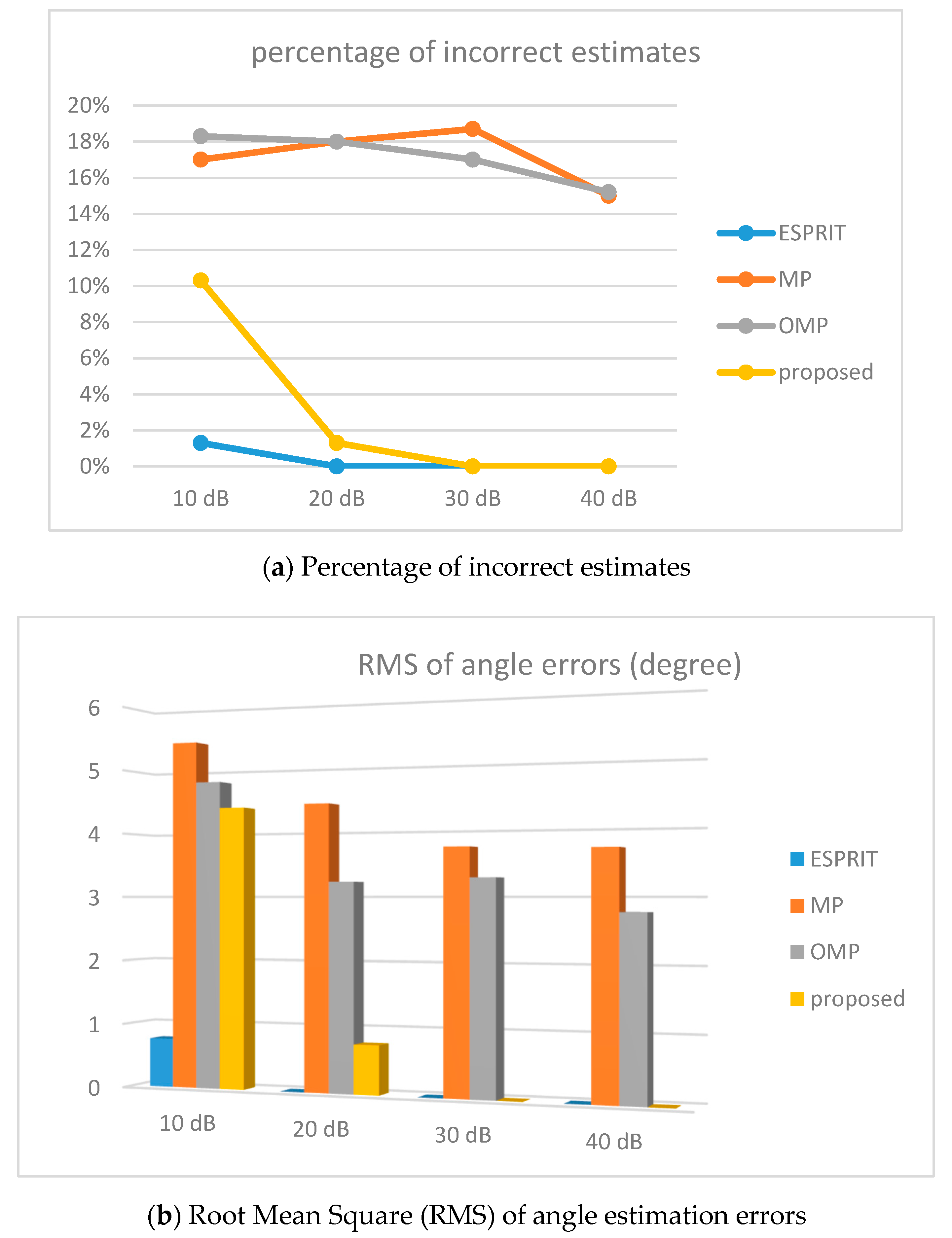
3.2. Simulation Results and Discussions

We first simulate the single signal source case. No estimation error occurs in all four schemes. This means DoA estimation problem for single signal source is less challenging and can be correctly carried out by all four schemes with a reasonable SNR setting, i.e., greater than 10 dB. For cases with multiple signal sources, the number K is first set to 3. In addition, the receiving powers of the three signal sources are different to mimic the scenario of different distances. The powers of the second and the third signal sources are 3 and 6 dB, respectively, lower than that of the first signal source. The simulation results for version 1 codebook are shown in Figure 6, where Figure 6a corresponds to the percentage of incorrect estimation and Figure 6b shows the RMS value of angle error. Among the 4 schemes, the ESPRIT scheme exhibits the best estimation accuracy and the estimation error can be reduced to zero if the SNR value is sufficiently large, i.e., above 20 dB. The result is not surprising because the ESPRIT scheme adopts a most complicated approach to achieve the accuracy. The proposed scheme is ranked in the second place and the error percentage and the RMS value dwindles rapidly as the SNR value increases. It can also achieve error free estimation when the SNR value reaches 30 dB. The benefit of signal sub-space approach stands out when the noise factor diminishes. In case of inferior SNR setting (10 dB), the percentage is 10.3%. However, in most cases, vectors neighboring to the correct one are selected, which means the estimation error is mostly less than 5°, the angular resolution of the codebook. This percentage also drops drastically as the SNR value improves. For the MP scheme, the error percentage ranges from 15% to 18.7% and does not decrease monotonically with the increase of SNR value. Further examination on the simulation results reveal that estimate errors occur most likely when the angular separation of two signal sources is smaller than the angular resolution of the codebook. The subtraction of the contribution from the selected vector performed in each iteration in the MP scheme may partially remove the signal from the second source. This can be considered as a “masking” effect. This effect is also true for the orthogonalization process performed in the OMP scheme. Another explanation is because the MP and OMP scheme employs a greedy and sequential search strategy. If the first match is incorrect, which happens most likely when none of signal sources has a dominant power over others, the error propagates to the subsequent matching process. The phenomenon of error propagation cannot be corrected through the orthogonalization process and is irrelevant to the SNR value. Note that the proposed scheme, after sub-space projection, employs a parallel matching strategy and is thus free of the error propagation problem. Although the error percentage of the OMP scheme reduce slightly with the SNR value, the trend of reduction is slow. In terms of the RMS value, the ESPRIT scheme still takes the lead. The RMS value of the proposed scheme is 4.39° when SNR = 10 dB, reduces to 0.76° when SNR reaches 20 dB, and finally becomes zero when SNR is 30 dB or larger. The OMP scheme performs slightly better than the MP scheme and the RMS value gradually reduces to less than 3°. For version 2 codebook, the simulation results are shown in Figure 7. Because of a smaller codebook with a coarser angular resolution, the error percentages and the RMS values of all DoA schemes or the proposed scheme improve significantly. For the ESPRIT scheme, it can achieve error free estimations. For the proposed scheme, errors only occur in the low SNR region is only 0.3% and the RMS value is roughly 0.4° and both subside quickly to zero when SNR value increases. The error percentages and the RMS values of both MP and OMP scheme also improve significantly using this version of codebook. This is because of the increased angular separation of two neighboring signal sources, which alleviates the masking effect in estimation.

We also conducted simulations on the cases of two signal sources (K = 2), the power of the second signal source is 3 dB lower than the first one. Since the estimation complexity decreases with the K value, only version 1 cookbook, a more challenging one, with a finer angular resolution is used in simulations. The results are shown in Figure 8. In terms of percentage of error estimates, The ESPRIT scheme is zero and the proposed scheme is almost error free except for the lowest SNR setting. Both MP and OMP schemes yield identical results in this simulations and error percentage drop from 8% to 5% as SNR value increases. The RMS of angle estimation errors, however, are confined to less than 1.4°. It is speculated that the effectiveness of the orthogonalization process adopted in OMP is more significant when there are more signal sources.

In conclusion, the proposed P²MP scheme outperform the two MP based schemes and can achieve an estimation performance close to that of the ESPRIT scheme but requires only a small fraction of the computing efforts.

3.3. Evaluation of K Value Selection

Recall that the number of signal source, K, is a priori information to the proposed P²MP scheme in constructing the $V_S$ matrix. In practice, this information could be either not available or incorrect. We will next evaluate how resilient the proposed scheme is to the accuracy of K value. We assume the correct number of signal sources is 3 and use different K values ranging from 1 to 8 to perform the DoA estimation. The antenna array size and the codebook (with 5° angular resolution) definition are identical to those used in the previous case of simulations. The power attenuations of the second and the third signal sources with respect to the first one are -7 and -10 dB, respectively. The larger the power attenuation is, the more difficult the DoA estimation becomes because the weakest signal source tends to be masked by the strongest one. The simulations are conducted by using two SNR settings, i.e., 20 and 10 dB.

Table 2. Evaluation of K value on the DoA estimation accuracy of the proposed scheme.

K Value		1	2	3	4	5	6	7	8
RMS of estimation error	SNR 20dB	29.1°	17.3°	0.67°	0.29°	0°	0°	0°	30°
	SNR 10dB	33.65°	23.7°	4.83°	3.53°	2.34°	0.91°	0.41°	31.83°
Percentage of incorrect matching	SNR 20dB	80.3%	58.3%	1.7%	1%	0%	0%	0%	90%
	SNR 10dB	60%	33.3%	12.6%	7.3%	3.7%	1.3%	0.7%	80.3%

summarize the simulation results based on 100 trials each. When the selection of K value is less than the correct number of signal sources, i.e., K = 1 or 2, the RMS values of estimation are considerably large in both SNR cases. In particular, the percentages of incorrect matching are well above 30%. This is because the constructed $V_S$ matrix is short in rank to span the signal sub-space properly. The larger the rank deficiency is, the worse the estimation performance becomes. When the K value reaches 3, it means the rank of $V_S$ matrix is equal to the number of signal sources and the RMS value of estimation errors reduces dramatically to less than 1 ° and 5° in SNR = 20 dB and SNR = 10 dB cases, respectively. The percentage of incorrect matching also drops to 1.7% and 12.6%, respectively. In the high SNR case, the estimation performance improves slightly as the K value increases to 4. When K equals 5, the estimation error diminishes to zero. When the K value reaches 8, i.e., the number of antennas N, $V_S$ equals $R_{xx}$. If $R_{xx}$ is full ranked, the noise sub-space is completely nullified, and the projection matrix $P_S$ becomes an identity matrix. In other words, no projection is performed and the accuracy of estimation degrades drastically. In the low SNR case, further increase in k value beyond 3 yields constant improvement. When k equals 7, the error percentage is only 0.7%. The trend of performance improvement with the increase of the K value can be explained as follows: In the proposed scheme, the first K columns of the $R_{xx}$ matrix are used to construct the $V_S$ matrix. Despite of its simplicity, these K vectors may not always span the signal sub-space faithfully, in particular in the low SNR cases. As more vectors added to the basis, the span would approximate the real signal sub-space provided the noise power is not significant. Actually, if the proper vectors are selected, K of them would be sufficient. This, however, requires extra computing efforts to select. In conclusion, if the K value falls between the correct number of signal sources and $N-1$, the estimation performance is guaranteed. This suggests the performance of the proposed scheme is rather robust to the K value selection. However, for low SNR applications, a larger K value is suggested to yield better results.

3.4. Detection Results of FMCW Radar

In this subsection, we will evaluate how the DoA estimation and beamforming affect the FMCW radar detection results. We will use Minimum Variance Distortionless Response (MVDR) beamforming technique [27] to combine the baseband signals received from 8 antennas. The weight vector can be calculated as

$$W_{MVDR}=\frac{R_{xx}^{-1}·h_0}{h_0^H{R}_{xx}^{-1}·h_0}$$

(8)

where $h_0$ is the steering vector found in DoA estimation. Follow the design sepcs defined in

Table 3. Specifications of the radar system and the design requirements of the DoA estimation.

Chirp Frequency Range	77 GHz~78 GHz	Max Beat Frequency	3.2 MHz
Bandwidth	1 GHz	Antenna array size	8
Sweep time	20μs	FoV	90°
Chirp rate	±1 G Hz/20 μs	Sweep angle Range	−45°~45°
Sampling rate	12.8 M Samples/s	Angular resolution	5°
Snapshots of Number	256 points	Codebook size	19
Maximum range	9.6 m	FFT size	256
DoA Estimation rate	One estimate per sweep	Maximum no. of targets	3

, Figure 9 shows the fast Fourier transform (FFT) spectrum of a single antenna signal when there are 3 signal sources located at 1.2 m, 1.8 m and 2.3 m away from the FMCW radar, respectively. The power attenuation is assumed to be proportional to the square of the distance. The SNR setting is 10 dB. There are three more prominent peaks indicating the distances of the three signal sources. Note that the third peak is not as significant as the first two and it is possible that this detection may fail. On the contrary, some noise spikes can be mistreated as the signal and cause false alarm. In Figure 10, three FMCW spectrums are shown and each one is the result of applying the MVDR beamforming using the steering vectors obtained from DoA estimation, respectively. Apparently, beamforming successfully suppresses the interference from other directions and simplify the peak detection efforts, provided the DoA estimation results are correct.

Although there are many Constant False Alarm Rate (CFAR) based FMCW signal detection schemes, for simplicity, we use the FindPeak function in MatLab with adjusted parameter setting to locate the beat frequencies. Table 3 summarizes the FMCW radar detection results with and without beamforming. The results cover two SNR values, i.e., 10 dB and 20 dB. For the non-beamforming case, only the distance matters. For the beamforming case (P²MP estimation + MVDR beamforming), a correct detection means both the arriving angle and the distance are correct. For SNR = 10 dB, the detection rate with beamforming can be boosted from 77.53% to 90.13%. The false alarm rate can be reduced to less than 1% as well. For SNR = 20 dB, the detection rate with beamforming can be further improved to 99.13%. The false alarm rate without beamforming is significantly lower in high SNR operations. Applying beamforming can further minimize this error rate. In

Table 4. FMCW detection results with and without beamforming.

Signal Source Number= 3, Codebook (−45°:5°:45°) Average Results Based on 500 Simulation Trials
SNR	10 dB			20 dB
Detection rate w/o beamforming	77.53%			77.93%
Detection rate for P2MP+MVDR beamforming	90.13%			99.13%
False alarm rate without beamforming	28.93%			2.73%
False alarm rate for P2MP+MVDR beamforming	0.87%			0.53%
Prominence Simulation	signal 1	signal 2	signal 3	signal 1	signal 2	signal 3
Average prominence of detected peaks w/o beamforming	53.71	23.44	9.44	53.32	22.65	9.37
Average prominence of detected peaks for P2MP+MVDR beamforming	218.71	85.11	28.97	204.49	86.21	46.62

, we also list the average "prominence" value of the detected peaks in the FFT spectrum. It is clear that beamforming can greatly enhance the prominence values of these peaks to facilitate better detection results.

4. Hardware Accelerator Design and Chip Implementation Results

Based on the presented DoA estimation scheme, an efficient hardware accelerator design is developed. The target application is a mm-wave Frequency Modulated Continuous Waveform (FMCW) radar system, which transmits a continuous wave signal with frequency varies linearly up and down within a specified period (sweep time). The frequency difference between the transmitted and received signals (beat frequency) is a constant, which is proportional to the time lap between the transmission and the reception of signal. The time lap equals the round trip time between the radar and the target and can be used to calculate the distance by multiplying with the light speed.

4.1. Design Specs and System Architecture

The specifications of the FMCW radar system equipped with an antenna array and the design requirements of the DoA estimation are listed in Table 3. The parameters crucial to the DoA estimation include antenna array size (N = 8), the codebook size (M = 19), the sweep time (20 μs), and the baseband signal sampling rate (12.8 MS/s). The goal is achieving one estimation per sweep. There are 256 samples in each sweep. Since the maximum detection range of this radar system is set to 9.6 m, the largest time lap between transmission and receiving is 64 ns. That is, the beat frequency would become stable 64 ns after the sweep starts. For a 12.8 MHz beat signal sampling rate, this interval is less than the sampling period, which is 78 ns. In other words, invalid data accounts for only 1 out of 256 sample vectors received in a chirp. Therefore, we did not drop the first sample vector deliberately and a 256-point FFT is performed to obtain the spectrum in range detection. One fourth of these samples, i.e., 64, are used for calculating the auto-correlation matrix. This also means the collection of 64 samples needed for auto-correlation matrix calculation would consume one fourth of the time budget available. What remains to be performed in a sweep includes DoA estimation, possible beamforming if required, and distance calculation. Therefore, the time budget for the DoA estimation is set to a quarter of the sweep time, as well. The maximum number of signal sources (targets), the K value, is set to 3. The target system clock rate is set to 8 times the sampling rate, which is 102.4 MHz. The number of the clock cycles available for the DoA estimation is thus 102.4 MHz × 5 μs = 512.

Figure 11 shows the system block diagram of the hardware design of the P²MP DoA estimation scheme. It contains four major building blocks, i.e., auto-correlation matrix calculation (AM), QR decomposition, projection matrix calculation (PM) and codebook search via matching pursuit (MP). Fixed point simulations are conducted first to evaluate the performance loss due to finite precision calculations and then determine the required word length for each module. The results are shown in Figure 12, where the three-tuple number associated with each module represents the sign bit, and the bit widths of the integral and fractional parts, respectively. The implementation loss in terms of the RMS value of estimation error is small than 1°.

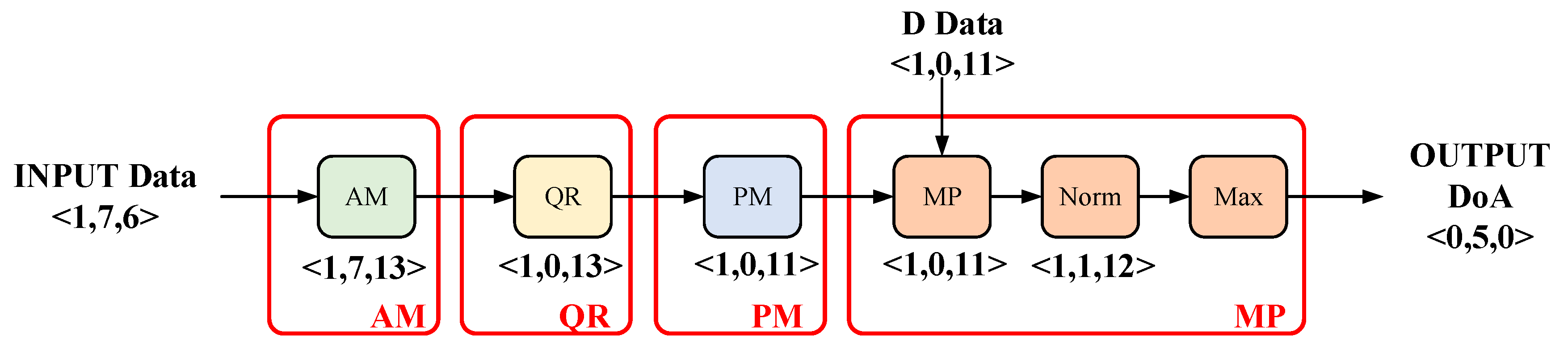
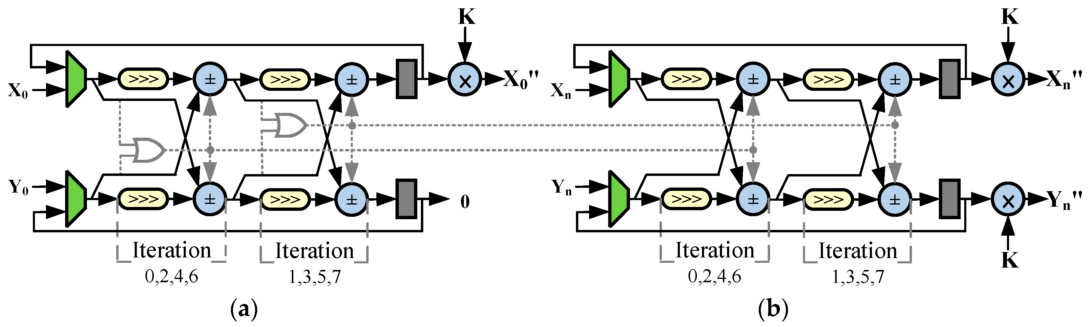
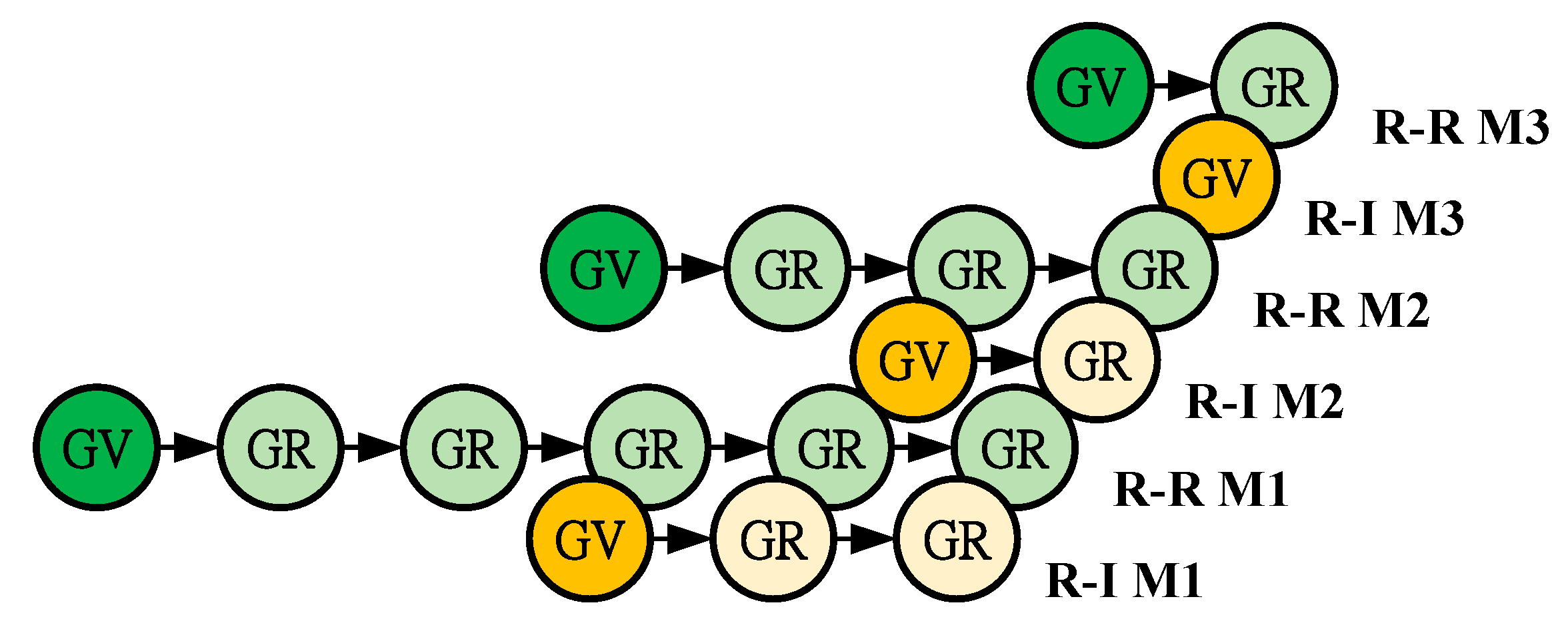
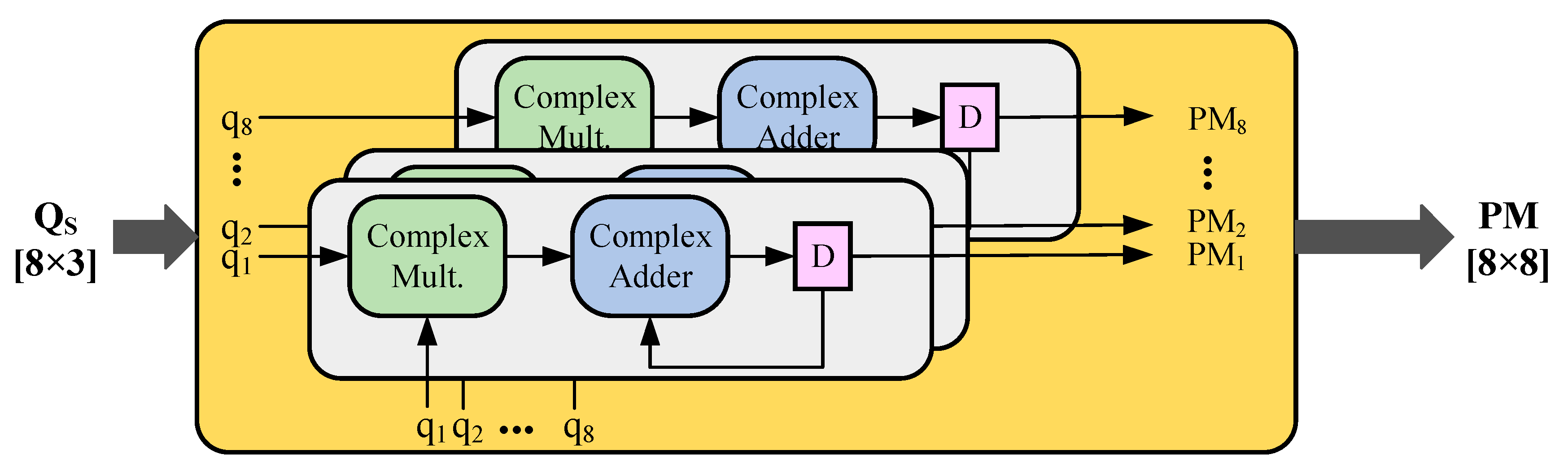
4.2. Algorithm Mapping and Module Designs

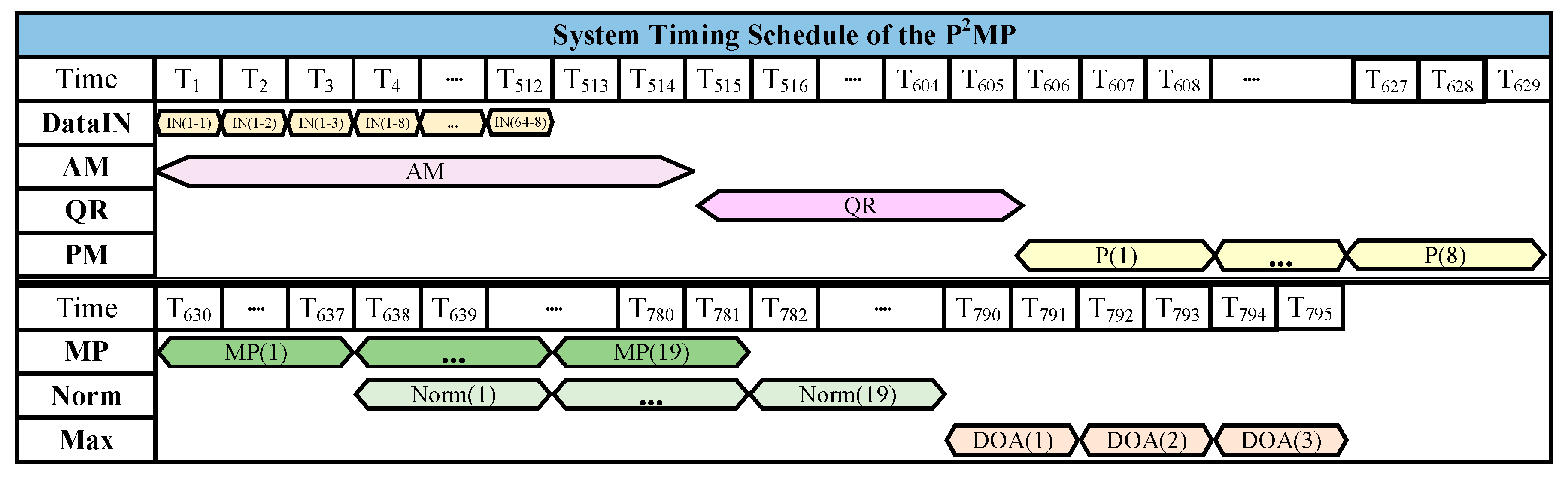
In the AM module, because the input data rate is bounded by the analog-to-digital conversion (ADC) sampling rate while the system clock rate runs 8 times higher, 8 data items acquired in each sampling are fed to the AM module in 8 consecutive clock cycles. An input delay line is employed to buffer the data. Figure 13 shows the systolic array design for the AM module by computing the outer-product of input vector and then then taking average. Only 3 (or K) sets of complex-valued Multiply-And-Accumulate (MAC) units are needed. Each MAC unit is responsible of computing one column of $R_{xx}$. The input delay line serves as a data pipeline passing input data from one MAC unit to another. Since only K columns of the $R_{xx}$ are required, the length of the delay line is K. Another set of registers taking the complex conjugate of input data are employed to hold another vector needed in outer product computations. One vector outer product can be performed every eight clock cycles and computations of 64 consecutive input vectors can be seamlessly chained together. It takes 64 × 8 + K-1 clock cycles to complete the $R_{xx}$ computations. The extra K-1 clock cycles arise because the operations of K MAC units are skewed by each skewed by one clock cycle. This meets the time budget as specified before.

The QR decomposition is the most complicated computing module. As described in Section 2.2, the decomposition is achieved by applying a sequence of Givens rotations, which involve trigonometric operations such as sine() and cosine(). Although there are various computing schemes, the Coordinate Rotation Digital Computer (CORDIC) scheme is adopted for its efficiency in hardware implementation. The CORDIC scheme computes various trigonometric functions by performing a sequence of micro-rotations iteratively using shift and add operations only. The number of iterations required is, in general, equal to the bit width of the desired data precision. A normalization process is needed in the final stage to restore the correct vector norm. This corresponds to a constant multiplication. In CORDIC, there are two computing modes. In the vector mode, the rotation nullifies one entry and turns the other to the norm 2 value of a 2-D vector. In the rotation mode, the vector is rotated subject to a specified angle. In QR decomposition, the vector mode is used when nullifying the leading element of a row while the rotation mode is applied when performing subsequent rotations in the same row. Note that the values rotation angle θ need not be computed directly. In the CORDIC scheme, it can be represented by a sequence of ±1 indicating the direction of each micro-rotation. Therefore, the leading vector mode CORDIC unit can simply pass the micro-rotation sequence to the trailing rotation mode CORDIC units in the same row. Figure 14 shows the CORDIC unit designs for vector and rotation modes, respectively. To reduce the number of clock cycles needed in the iterative process, two micro-rotations are performed per clock cycle. Fixed point simulation results indicate 8 iterations are sufficient to achieve the required data precision. In total, four plus one clock cycles are needed to perform a 2 × 2 real-valued Givens rotation. The extra one is for the normalization.

After elaborating the basic function unit CORDIC, the systolic architecture of the QR decomposition is presented. As illustrated in Figure 15, the QR module consists of a triangular systolic array followed by a rectangular one. The triangularization of the $V_S$ matrix is performed in the triangular systolic array, where each circle indicates a Processing Element (PE) for complex-valued Givens rotation. As stated before, one complex-valued Givens rotation is implemented by three real-valued Givens rotation. Therefore, each PE design consists of three CORDIC units. The sized 8 × 3 $V_S$ matrix is admitted from the bottom of the triangular array and the columns of the resultant R matrix are obtained at the PEs along hypotenuse. The $Q_S$ matrix is calculated in a rectangular array containing 8 × 3 PEs. A sized 8 × 8 identity matrix is fed to the array from the bottom and the $Q_S$ matrix is available at the top of the array. The leading PE in each row operates in the vector mode and passes the micro-rotations sequence to the downstream PEs, all operating in the rotation mode. Figure 16 shows a detailed systolic triangular array design for R matrix calculation after substituting each complex-valued PE with three CORDIC units. Label “GV” means vector mode operation and label “GR” means rotation mode operation. For the label at the right end of each row, “R-I” means the CORDIC units in this row is responsible for converting the operand to real-valued by eliminating its imaginary part. Label “R-R” means the Givens rotation for the two converted (to real-valued) operands. The detailed design of the rectangular array can be likewise derived.

The PM module performs a matrix multiplication to obtain the projection matrix. As shown in Figure 17, the design is a linear systolic array that consists of eight complex-valued MACs. The $Q_S$ matrix is inputted to the module column by column in three consecutive clock cycles and a column of the P matrix is obtained every three clock cycles. For the Matching pursuit module, the projection of the codebook, i.e., $\Psi =D^H·P_S$ is performed first. The codebook need to store 19 steering vectors and each vector is 8-dimensional with 24-bit complex-valued entries (12-bit for real part and 12-bit for imaginary part). The total memory size is only 456 bytes. Although we can use memory compiler to generate a small on-chip SRAM module for it, to support computing parallelism, these data are stored in registers so that they can be accessed in parallel. The projection is, again, a matrix-matrix multiplication and differs from the counterpart in the PM module only in matrix size. A similar linear systolic array design with eight MACs is adopted here. However, it takes 8 clock cycles to complete the projection of one steering vector from the codebook and there are 19 vectors in total. The norm 2 value of each projected vector is next calculated. Since this value is used in the magnitude comparison process, the square of the norm 2 value is calculated instead to eliminate square root operations. As there are eight clock cycles for the magnitude comparison, a single complex-valued MAC unit would meet the timing demands. The next maximal K value selection can be easily implemented by chaining 3 (or K) comparators. Finally, the indexes of the K largest steering vectors are exported.

4.3. System Timing

Figure 18 depicts the timing diagram of the overall hardware accelerator design. The first 512 plus two clock cycles are allotted for the auto-correlation matrix. This latency is actually bounded by the input data rate, which takes 512 clock cycles to admit 64 sample vectors. The AM module spends just two more clock cycles to complete computations after all input data are available. The QR module consumes 91 clock cycles to generate R and $Q_S$ matrices. The PM module spends another 8 × 3 clock cycles to compute the projection matrix. The MP module completes the projection of a steering vector every eight clock cycles. The projected vector is immediately passed to next unit to compute its norm 2 square value. The vector projections and the norm 2 square value calculations are performed in the same pace to form a two-stage computing pipeline. In the final phase, it takes six clock cycles to do the sorting and output the indexes of the estimation results. In total, it takes 795 clock cycles to complete the auto-correlation matrix calculation and DoA estimation. Taking the AM calculation part away, the DoA estimation itself requires 283 clock cycles. This meets the design specs that the estimation should be completed within 512 clock cycles (5 μs).

4.4. Chip Design

The hardware accelerator design is coded in Verilog and synthesized by using the Synopsys Design Compiler tool. An ARM standard cell library is adopted in the backend design and the target implementation technology is a 40nm TSMC CMOS process. Figure 19 shows the final layout view accomplished by using Synopsys IC Compiler. The accelerator chip design details are summarized in

Table 5. Accelerator chip design summary.

Item	Specification
Technology process	TSMC 40 nm CLN 40 G
Cell library	ARM Cell-based Design Kit
Voltage (Core/IO)	0.9/3.3 V
Maximum clock frequency	333 MHz
Minimum clock period	3ns
Core Size	0.76 ${\mathrm{mm}}^2$
Die Size	2.61 ${\mathrm{mm}}^2$
IO Pad	75
Gate Count	454.4 k
Power (Chip/Core)	177/83 mW
Latency	512 (auto-correlation matrix) + 283 (DoA estimation) Cycles
Initiation interval	1.536 μs (512clock cycles)
Throughput	1.18 M estimates/sec

, where layout area, gate count and power consumption are based on the report from IC Compiler. The timing information is obtained from the PrimeTime-PX tool. The total chip die size is 2.61 ${\mathrm{mm}}^2$, while the internal core design occupies an area of 0.76 ${\mathrm{mm}}^2$. The core design is roughly divided into four parts, i.e., MP (matching pursuit), QRD, PM (Projection Matrix) and AM (Auto-correlation Matrix), using different colors. The equivalent gate count in total is 454.4 k. Figure 20 shows the breakdown of hardware complexity measured in gate count. Among these function units, QRD is the most complex one and accounts for one half (49.9%) of the total gate count. MP is ranked in the second place and consumes 30.9% of the total gate count. AM and PM are of similar complexities and the percentages are 8.4% and 7.6%, respectively. The remaining 3.2% is attributed to the I/O buffer. The clock rate of the core design can reach 333MHz and the corresponding power consumptions for the core design is 83mW. The total DoA estimation takes 795 (= 512 + 283) clock cycles. Note that the first 512 clock cycles are actually bounded by the time span needed to collect 64 input samples for auto-correlation matrix calculation. The remaining 283 clock cycles are dedicated to DoA estimation. The original time budget is 10 μs (1024 clock cycles @102.4MHz). The implementation result is 2.4 μs (795 clock cycles @333MHz). If we exclude the AM calculation part, the estimation itself requires only 0.85 μs. This suggests a throughput rate of 1.18 M estimates/sec.

4.5. Comparison with Other DoA Hardware Implementation Works

Regarding the hardware design efficiency of the proposed work, our literature survey cannot identify any other work with chip design. However, there have been works [28,29,30,31] with hardware implementations reported in recent years and all of them are using the FPGA technology. In industry practices, FPGA is usually employed in the cases of system prototyping or when product volume is not large enough to economically justify the Application Specific Integrated Circuit (ASIC) implementation. The design efforts and the NRE (Non-Recurring Engineering) cost of ASIC are significantly higher than those of the FPGA. The unit cost of ASIC, once the economical volume is reached, however, can be lower than that of FPGA. In this paper, we choose the ASIC approach simply to demonstrate how DSP intensive applications can benefit from a carefully crafted ASIC design in terms of speed and throughput.

Table 6. Performance comparison of related DoA estimation hardware implementations.

	[28]	[29]	[30]	[31]		This Work
estimation scheme	Bartlett	MUSIC	LU decomp. ESPRIT	LDL decomp.	Cholesky Decomp.	Projection and parallel MP
Antenna array size	$1\times 4$	$1\times 8$	$1\times 4$	$1\times 4$	$1\times 4$	$1\times 8$
Norm. problem complexity	1/8	1	1/8	1/8	1/8	1
Implementation	FPGA	FPGA	FPGA	FPGA	FPGA	ASIC
Design effort	medium	medium	medium	medium	medium	high
NRE cost	medium	medium	medium	medium	medium	high
Unit cost	medium	medium	medium	medium	medium	low
Input word length	8 bits	16 bits	20 bits	20 bits	20 bits	21 bits
Clock Rate	225 MHz	160 MHz	56.47 MHz	52.5 MHz	54.3 MHz	333 MHz
Circuit complexity	NA	54,100 LUTs 64 DSP48s	23,438 LUTs 10 BRAMs 265 DSP48s	21,870 LUTs 10 BRAMs 233 DSP48s	21,956 LUTs 10 BRAMs 230 DSP48s	454.4 k gates
Initiation interval	0.804μs	93.4μs	2.82μs	3.77μs	4.05μs	1.536μs
Throughput (estimates/sec)	1.24 M	10.7 K	0.36 M	0.27 M	0.25 M	0.65 M
Latency (cycles)	181	14,944	159	198	220	512+283
Norm. latency	1448	14,944	1272	1584	1760	795

lists the design indexes of the proposed work and five other designs. In this table, we list the DoA estimation scheme, antenna array size, input word length, clock rate, latency, initiation interval and throughput results associated with each design. Note that there are various factors affecting the implementation results. These include the antenna array size (or the problem size), the adopted estimation algorithm complexity, the accuracy of estimation, the maximum number of signal sources, the codebook size, the hardware complexity, the implementation technology, and so on. It is, thus, not likely to come out with a leveled index taking every factor into account. Therefore, the comparison emphasizes on the merits of hardware design and does not consider the discrepancy in algorithm complexity and estimation accuracy. However, some basic normalization measures are adopted for a fair comparison. First of all, the computing latency is measured in terms of clock cycles rather than the absolute time span. This can effectively eliminate the factor of implementation technology. Secondly, the generic problem complexity is considered. Despite the differences in DoA estimation schemes, all of them bear a algorithm complexity of order N³, where N is the antenna array size. We set the problem complexity of N = 8 as 1 and the problem complexity of N = 4 becomes 1/8. This leads to a normalized latency by taking the problem complexity into account.

From Table 6, design [29] and the proposed work target a 1 × 8 antenna array while the remaining four use a 1 × 4 antenna array. This means the problem complexity of a 1 × 4 antenna array is roughly one eighth that of a 1×8 antenna array. As for the input word length, which may affect the width of data path design, most designs adopt word length between 16 and 21 bits. The reported clock rates vary from 52.5 MHz (design [31]) to 333 MHz (the proposed work). FPGA, because of its programmable feature and a lot of logic overhead, can barely meet the speed achieved by ASIC. The hardware complexity, although listed in the comparison table, is not compared because there is no credible complexity conversion formulas between FPGA and ASIC technologies. Note that BRAM and DSP48 in FPGA implementations indicate embedded memory module and hardwired multiplier, respectively. The latency is measured as number of clock cycles, regardless of the clock rate, needed to complete the estimation. This latency includes both the time spent in auto-correlation matrix calculation and the time to perform DoA estimation. From Table 6, designs [28,30,31] all can accomplish the estimation in less than 220 clock cycles. This is because they work on a smaller antenna array. The proposed design takes 512 clock cycles in calculating the auto-correlation matrix and another 283 clock cycles in performing the estimation. The total latency is thus 795 clock cycles. Note that in our design, the auto-correlation matrix calculation is performed in pace with the data input rate. This is considered an input rate constrained design and the hardware circuitry is minimized to just meet the throughput requirement. It takes 512 clock cycles to collect the needed 64 sample vectors and, in the mean time, calculates the auto-correlation matrix incrementally. Once all sample vectors are admitted, it actually spends two additional clock cycles only to wrap up the entire auto-correlation matrix calculation. If we take the problem complexity into consideration, the normalized latency of the proposed design is the shortest one in all designs. The initiation interval indicates the time interval between two successive DoA estimations and its reciprocal corresponds to the throughput. For the proposed design, the auto-correlation matrix calculation module and the remaining computing modules can work in parallel. Therefore, the initiation interval is bounded by the latency of auto-correlation matrix calculation. This corresponds to a 1.536 μs interval when the clock rate is 333 MHz. The corresponding throughput is thus 0.65 M estimates/sec. Except for design [29], all other designs have successfully confined their initiation intervals to less than 4 μs. Design [29] uses relatively fewer FPGA resources than other FPGA based design. It also deals with a 1 × 8 rather than a 1 × 4 antenna array. That may explain why it has the largest initiation interval (lowest throughput) among all designs. Design [28], due to its smaller problem complexity and a much smaller data path width, shows the highest throughput rate. In summary, this table provides an overview of how DoA estimation algorithms are implemented in hardware. Most of these hardwired designs can initiate a new estimation in just a few micro-seconds, which are much faster than the software based designs can achieve, usually measured in the unit of mili-seconds. The proposed design also features the shortest normalized latency.

5. Conclusions

In conclusion, an efficient DoA estimation scheme and its hardware accelerator design in chip implementation is presented in this paper. The proposed scheme features a combination of signal sub-space projection and parallel matching pursuit techniques, i.e., applying signal projection first before performing matching pursuit from a codebook. This measure helps minimize the interference from noise sub-space and makes the matching process free of extra orthogonalization computations. It thus exhibits the lowest computing complexity and the second best estimation accuracy among the schemes under comparison. We also evaluate the impact of K value selection on the estimation accuracy and demonstrate how this DoA estimation scheme improves the FMCW radar detection. After algorithm performance verifications, the corresponding hardware accelerator chip design is also developed and can accomplish one multiple-source (up to 3) DoA estimation every 1.536 μs, which indicates a processing throughput as high as 0.65 M estimates per second. Hardware design comparison with 5 other related works is also conducted. Although the comparison result is not conclusive due to the discrepancy in many design factors, the proposed design excels others in that it spends the fewest clock cycles (after normalization) in performing the estimation.

References

1. Petre, S.; Nehorai, A. MUSIC, maximum likelihood, and Cramer-Rao bound. IEEE Trans. Acoust. Speech Signal Process. 1989, 37, 720–741. [Google Scholar]
2. Yan, F.; Jin, M.; Qiao, X. Low-complexity DOA estimation based on compressed MUSIC and its performance analysis. IEEE Trans. Signal Process. 2013, 61, 1915–1930. [Google Scholar] [CrossRef]
3. Ali, H.; Shubair, R.M.; Salahat, E. Enhanced DOA estimation algorithms using MVDR and MUSIC. In Proceedings of the IEEE International Conference on Current Trends in Information Technology (CTIT), Dubai, United Arab Emirates, 11–12 December 2013. [Google Scholar]
4. Rao, B.D.; Hari, K.V.S. Performance analysis of root-MUSIC. IEEE Trans. Acoust. Speech Signal Process. 1989, 37, 1939–1949. [Google Scholar] [CrossRef]
5. Marius, P.; Gershman, A.B.; Haardt, M. Unitary root-MUSIC with a real-valued eigen decomposition: A theoretical and experimental performance study. IEEE Trans. Signal Process. 2000, 48, 1306–1314. [Google Scholar]
6. Tanaka, A.; Imai, H. MUSIC-Based DoA Estimation by Oblique Projection along the signal sub-space. In Proceedings of the IEEE Workshop on Statistical Signal Processing (SSP), Gold Coast, Australia, 29 June–2 July 2014. [Google Scholar]
7. Richard, R.; Kailath, T. ESPRIT-estimation of signal parameters via rotational invariance techniques. IEEE Trans. Acoust. Speech Signal Process. 1989, 37, 984–995. [Google Scholar]
8. Sylvie, M.; Marsal, A.; Benidir, M. The propagator method for source bearing estimation. Signal Process. 1995, 42, 121–138. [Google Scholar]
9. Zheng, G.; Chen, B.; Yang, M. Unitary ESPRIT algorithm for bistatic MIMO radar. Electron. Lett. 2012, 48, 179–181. [Google Scholar] [CrossRef]
10. Lin, J.; Ma, X.; Yan, S.; Hao, C. Time-Frequency Multi-Invariance ESPRIT for DOA Estimation. IEEE Antennas Wirel. Propag. Lett. 2016, 15, 770–773. [Google Scholar] [CrossRef]
11. Zhang, W.; Han, Y.; Jin, M.; Li, X.-S. An Improved ESPRIT-Like Algorithm for Coherent Signals DOA Estimation. IEEE Commun. Lett. 2020, 24, 339–343. [Google Scholar] [CrossRef]
12. Mallat, S.; Zhang, Z. Matching pursuit with time-frequency dictionaries. IEEE Trans. Signal Process. 1994, 41, 3397–3415. [Google Scholar] [CrossRef] [Green Version]
13. McClure, M.R.; Carin, L. Matching pursuits with a wave-based dictionary. IEEE Trans. Signal Process. 1997, 45, 2912–2927. [Google Scholar] [CrossRef]
14. Karabulut, G.; Kurt, T.; Yongaçoglu, A. Estimation of directions of arrival by matching pursuit (EDAMP). Eurasip J. Wirel. Commun. Netw. 2005, 2005, 618605. [Google Scholar] [CrossRef] [Green Version]
15. Tropp, J.; Gilbert, A.C. Signal recovery from random measurements via orthogonal matching pursuit. IEEE Trans. Inf. Theory 2007, 53, 4655–4666. [Google Scholar] [CrossRef] [Green Version]
16. Zhang, X.; Li, Y.; Yuan, Y.; Jiang, T.; Yuan, Y. Low-Complexity DOA Estimation via OMP and Majorization-Minimization. In Proceedings of the 2018 IEEE Asia-Pacific Conference on Antennas and Propagation (APCAP), Auckland, New Zealand, 5–8 August 2018. [Google Scholar]
17. Nasu, T.; Kikuma, N.; Sakakibara, K. Performance Improvement of DOA Estimation Using Conjugate Gradient Method with Subtraction Scheme. In Proceedings of the 2018 IEEE International Workshop on Electromagnetics: Applications and Student Innovation Competition (iWEM), Nagoya, Japan, 29–31 August 2018. [Google Scholar]
18. Wang, W.; Wu, R. High Resolution Direction of Arrival (DOA) Estimation Based on Improved Orthogonal Matching Pursuit (OMP) Algorithm by Iterative Local Searching. Sensors 2013, 13, 11167–11183. [Google Scholar] [CrossRef]
19. Aghababaiyan, K.; Shah-Mansouri, V.; Maham, B. High-Precision OMP-Based Direction of Arrival Estimation Scheme for Hybrid Non-Uniform Array. IEEE Commun. Lett. 2020, 24, 354–357. [Google Scholar] [CrossRef]
20. Wilkinson, J.H.; Bauer, F.L.; Reinsch, C. Linear Algebra. In Handbook for Automatic Computation (2); Springer: Berlin/Heidelberg, Germany, 1971; ISBN 978-3-662-39778-7. [Google Scholar]
21. Tang, C.F.T.; Liu, K.J.R.; Tretter, S.A. On systolic arrays for recursive complex Householder transformations with applications to array processing. In Proceedings of the IEEE Acoustics, Speech, and Signal Processing, Toronto, ON, Canada, 14–17 April 1991; pp. 1033–1036. [Google Scholar]
22. Chung, K.-L.; Yan, W.-M. The complex Householder transform. IEEE Trans. Signal Process. 1997, 45, 2374–2376. [Google Scholar] [CrossRef]
23. Lin, K.-H.; Chang, R.C.-H.; Lin, H.-L.; Wu, C.-F. Analysis and Architecture Design of a Downlink M-Modification MC-CDMA System Using the Tomlinson–Harashima Precoding Technique. IEEE Trans. Veh. Technol. 2008, 57, 1387–1397. [Google Scholar]
24. Singh, C.K.; Prasad, S.H.; Balsara, P.T. VLSI Architecture for Matrix Inversion using Modified Gram-Schmidt based QR Decomposition. In Proceedings of the International VLSI Design Conference, Bangalore, India, 6–10 January 2007; pp. 836–841. [Google Scholar]
25. Hwang, Y.-T.; Chen, W.-D. Design and Implementation of a High Throughput Fully-Parallel Complex-Valued QR Factorization Chip. IET Circ. Devices Syst. 2011, 5, 424–432. [Google Scholar] [CrossRef]
26. Richards, M. Fundamentals of Radar Signal Processing; McGraw-Hill: New York, NY, USA, 2005. [Google Scholar]
27. Zaharov, V.; Teixeira, M. SMI-MVDR beamformer implementations for large antenna array and small sample size. IEEE Trans. Circ. Syst. I Reg. Pap. 2008, 55, 3317–3327. [Google Scholar] [CrossRef]
28. Unlersen, F.M.; Yaldiz, E.; Imeci, S.T. FPGA based fast Bartlett, “DoA estimator for ULA antenna using parallel computing”. Appl. Comput. Electromagn. Soc. J. 2018, 33, 450–459. [Google Scholar]
29. Yan, J.; Huang, Y.; Xu, H.; Vandenbosch, G.A.E. Hardware acceleration of MUSIC based DoA estimator in MUBTS. In Proceedings of the 8th European Conference Antennas Propag (EuCAP), The Hague, The Netherlands, 6–11 April 2014; pp. 2561–2565. [Google Scholar]
30. Hussain, A.A.; Tayem, N.; Butt, M.O.; Soliman, A.-H.; Alhamed, A.; Alshebeili, S. FPGA Hardware Implementation of DOA Estimation Algorithm Employing LU Decomposition. IEEE Access 2018, 6, 17666–17680. [Google Scholar] [CrossRef]
31. Hussain, A.A.; Tayem, N.; Soliman, A.-H.; Radaydeh, R.M. FPGA-Based Hardware Implementation of Computationally Efficient Multi-Source DOA Estimation Algorithms. IEEE Access 2019, 7, 88845–88858. [Google Scholar] [CrossRef]
Figure 1. Pseudo code of the Estimation of Signal Parameters Via Rotational Invariance Techniques (ESPRIT) Direction of Arrival (DoA) estimation algorithm.
Electronics 09 00641 g001
Figure 2. Combined pseudo code of the Matching Pursuit/Orthogonal Matching Pursuit (MP/OMP) DoA estimation algorithms.
Electronics 09 00641 g002
Figure 3. Pseudo code of the projection and parallel matching pursuit based DoA estimation algorithm.
Electronics 09 00641 g003
Figure 4. Pseudo code of Givens rotation based QR decomposition.
Electronics 09 00641 g004
Figure 5. Computing complexity comparisons of different (K, N, M) parameter combinations.
Electronics 09 00641 g005
Figure 6. Estimation performance comparisons for K = 3 using codebook version 1 (M = 19 and 5° angular resolution).
Electronics 09 00641 g006
Figure 7. Estimation performance comparisons for K = 3 using codebook version 2 (M = 10 and 10° angular resolution). (a) Percentage of incorrect estimates; (b) RMS of angle estimation errors.
Electronics 09 00641 g007
Figure 8. Estimation performance comparisons for K = 2 using codebook version 1 (M = 19 and 5° angular resolution). (a) Percentage of incorrect estimates; (b) RMS of angle estimation errors.
Electronics 09 00641 g008
Figure 9. FFT spectrum of Frequency Modulated Continuous Waveform (FMCW) radar signal from a single antenna.
Electronics 09 00641 g009
Figure 10. FFT spectrums of FMCW radar signal after applying Minimum Variance Distortionless Response (MVDR) beamforming.
Electronics 09 00641 g010
Figure 11. System block diagram of the DoA estimation hardware accelerator design.
Electronics 09 00641 g011
Figure 12. Word length specs for the computing modules.
Electronics 09 00641 g012
Figure 13. Systolic array design of the AM module.
Electronics 09 00641 g013
Figure 14. CORDIC unit designs. (a) vector mode; (b) rotation mode.
Electronics 09 00641 g014
Figure 15. Systolic array design of the QR decomposition module.
Electronics 09 00641 g015
Figure 16. Systolic tri-array design for R matrix using real-valued Coordinate Rotation Digital Computer (CORDIC) units.
Electronics 09 00641 g016
Figure 17. Linear systolic array design for the PM module.
Electronics 09 00641 g017
Figure 18. System Timing chart of the P2MP DoA estimation Hardware Design.
Electronics 09 00641 g018
Figure 19. Layout of the proposed DoA estimation accelerator chip design.
Electronics 09 00641 g019
Figure 20. Logic complexity breakdown of chip design.
Electronics 09 00641 g020