Abstract
The evaluation of kidney biopsies performed by expert pathologists is a crucial process for assessing if a kidney is eligible for transplantation. In this evaluation process, an important step consists of the quantification of global glomerulosclerosis, which is the ratio between sclerotic glomeruli and the overall number of glomeruli. Since there is a shortage of organs available for transplantation, a quick and accurate assessment of global glomerulosclerosis is essential for retaining the largest number of eligible kidneys. In the present paper, the authors introduce a Computer-Aided Diagnosis (CAD) system to assess global glomerulosclerosis. The proposed tool is based on Convolutional Neural Networks (CNNs). In particular, the authors considered approaches based on Semantic Segmentation networks, such as SegNet and DeepLab v3+. The dataset has been provided by the Department of Emergency and Organ Transplantations (DETO) of Bari University Hospital, and it is composed of 26 kidney biopsies coming from 19 donors. The dataset contains 2344 non-sclerotic glomeruli and 428 sclerotic glomeruli. The proposed model consents to achieve promising results in the task of automatically detecting and classifying glomeruli, thus easing the burden of pathologists. We get high performance both at pixel-level, achieving mean F-score higher than 0.81, and Weighted Intersection over Union (IoU) higher than 0.97 for both SegNet and Deeplab v3+ approaches, and at object detection level, achieving 0.924 as best F-score for non-sclerotic glomeruli and 0.730 as best F-score for sclerotic glomeruli.
1. Introduction
The spread of Deep Learning (DL) techniques and frameworks has led to a revolution in the medical imaging field. The assessment of organ viability, by donor kidney biopsy examination, is essential prior to transplantation. The traditional evaluation of biopsies was based on the visual analysis by trained pathologists of biopsy slides using a light microscope which is a time consuming and highly variable procedure. The high variability between the observers resulted in poor reproducibility among pathologists, which may cause an inappropriate organ discard. Therefore, the development of new techniques able to objectively and rapidly interpret donor kidney biopsy to support pathologist’s decision making is strongly fostered. The increasing availability of whole-slide scanners, which facilitate the digitization of histopathological tissue, led to a new research field denoted as digital pathology and generated a strong demand for the development of Computer-Aided Diagnosis (CAD) systems. As stated in the literature, the application of deep learning techniques for the analysis of Whole-Slide Images (WSIs) has shown significant results and suggest that the integration of DL framework with CAD systems is a valuable solution.
In the realm of digital pathology, several recent studies have proposed CAD systems for glomerulus identification and classification in renal biopsies [1,2,3,4,5,6,7,8]. The eligibility for transplantation of a kidney retrieved from Expanded Criteria Donors (ECD) relies on rush histological examination of the organ to evaluate suitability for transplant [9]. The Karpinski score is based on the microscopic examination of four compartments: glomerular, tubular, interstitial and vascular, in order to assess the degree of chronic injury. For each compartment is assigned a score from 0 to 3 where 0 corresponds to normal histology and 3 to the highest degree of, respectively, global glomerulosclerosis, tubular atrophy, interstitial fibrosis and arterial and arteriolar narrowing [9,10]. The evaluation of global glomerulosclerosis requires detection and classification of all the glomeruli present in a kidney biopsy, distinguishing between healthy (non-sclerotic) and non-healthy (sclerotic) ones.
The two fundamental components that characterize a non-sclerotic glomerulus are the capillary tuft with the mesangium and the Bowman’s capsule. The first one is placed inside the glomerulus while the second one is peripheral and has the function to contain the tuft. The space between these two components is called Bowman’s space. From a morphological point of view, the non-sclerotic glomerulus generally has an elliptic form. The capillary tuft has a pomegranate form, caused by the contemporary presence of blue points (nuclei of cells), white areas (capillary lumens) and variable amount of regions with similar tonality and different levels of saturation (mesangial matrix). A non-healthy glomerulus, from the point of view of Karpinski’s score, is a globally sclerotic glomerulus, namely a glomerulus where capillary lumens are completely obliterated for increase in extracellular matrix and Bowman’s space is completely filled by collagenous material. Examples of non-sclerotic and sclerotic glomeruli are depicted in Figure 1.
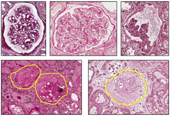
Figure 1.
Glomeruli. Top row: non-sclerotic glomeruli. Bottom row: sclerotic glomeruli.
Ledbetter et al. proposed a Convolutional Neural Network to predict kidney function (evaluated as the quantity of primary filtrate that passes from the blood through the glomeruli per minute) in chronic kidney disease patients from whole-slide images of their kidney biopsies [3]. Gallego et al. proposed a method based on the pretrained AlexNet model [11] to perform glomerulus classification and detection in kidney tissue segments [2]. Gadermayr et al. focused on the segmentation of the glomeruli. The authors proposed two different CNN cascades for segmentation applications with sparse objects. They applied these approaches to the glomerulus segmentation task and compared them with conventional fully convolutional networks, coming to the conclusion that cascade networks can be a powerful tool for segmenting renal glomeruli [4]. Temerinac-Ott et al. compared the performance between a CNN classifier and a support-vector machines (SVM) classifier which exploits features extracted by histogram of oriented gradients (HOG) [12] for the task of glomeruli detection in WSIs with multiple stains, using a sliding window approach. The obtained results showed that the CNN method outperformed the HOG and SVM classifier [1]. Kawazoe et al. faced the task of glomeruli detection in multistained human kidney biopsy slides by using a Deep Learning approach based on Faster R-CNN [6]. Marsh et al. developed a deep learning model that recognizes and classifies sclerotic and non-sclerotic glomeruli in whole-slide images of frozen donor kidney biopsies. They used a Fully Convolutional Network (FCN) followed by a blob-detection algorithm [13], based on Laplacian-of-Gaussian, to post-process the FCN probability maps into object detection predictions [8]. Ginley et al. proposed a CAD to classify renal biopsies of patients with diabetic nephropathy [7], using a combination of classical image processing and novel machine learning techniques. Hermsen et al. adopted CNNs, namely an ensemble of five U-Nets, for segmentation of ten tissue classes from WSIs of periodic acid-Schiff (PAS) stained kidney transplant biopsies [14].
The analysis of the literature suggests that main works focused on the glomerular detection task only, without considering the further classification into sclerotic and non-sclerotic [1,2,4,6]. Few papers considered the assessment of global glomerulosclerosis from kidney biopsies [7,8,14].
In our previous works we focused on other kidney biopsies analysis tasks, such as classification of tubules and vessels [15] and classification of non-sclerotic and sclerotic glomeruli [5]. In this work, we propose a CAD system to address the segmentation and the classification tasks of glomeruli, in order to obtain a reliable estimate of Karpinski histological score. The proposed work allowed us to obtain better results than the literature in the classification task.
2. Materials
The kidney biopsies dataset analyzed in this paper has been provided by the Department of Emergency and Organ Transplantations (DETO) of the Bari University Hospital. Slides were digitized using a high-resolution whole-slide scanner with a scanning objective which has a 20× magnification corresponding to a resolution of 0.50 μm/pixel. All the biopsies provided by DETO clinicians are PAS stained sections from formalin fixed paraffin embedded tissue. The complete dataset is composed of 26 kidney biopsies coming from 19 donors. It contains 2344 non-sclerotic glomeruli and 428 sclerotic glomeruli. The dataset has been split into a train-validation (trainval) set and a test set. The trainval set has been further split into a train set and a validation set; the last one is used for tuning hyperparameters and for assessing the trend of the loss function and of accuracy during the training process. A detailed overview of the dataset is reported in Table 1.

Table 1.
Dataset info.
3. Methods
3.1. Semantic Segmentation Framework
Convolutional Neural Networks have had a widespread adoption in all kinds of image analysis tasks, starting from AlexNet which won ImageNet Large Scale Visual Recognition Challenge 2012 (ILSVRC 2012) [16] by a huge margin [11], though pioneering work was already done by LeCun much earlier for handwritten digit recognition [17].
Semantic segmentation is a task which consists of classifying all the pixels belonging to an input image. In order to accomplish this task, most CNN semantic segmentation architectures are based on encoder-decoder networks. The encoder is devoted to the feature extraction process, shrinking the spatial dimensions while increasing the depth. The decoder has the task to recover the spatial information from the output of the encoder. Due to the several application in the medical imaging field, in this work we considered two main approaches based on SegNet and DeepLab v3+ architectures. The main SegNet applications regard segmentation tasks such as semantic segmentation of prostate cancer [18], gland segmentation from colon cancer histology images [19] and brain tumor segmentation from multi-modal magnetic resonance images [20]. DeepLab v3+ has been used for the semantic segmentation of colorectal polyps [21] and the automatic liver segmentation [22,23].
SegNet is a CNN architecture for semantic segmentation proposed by researchers at University of Cambridge [24]. As other semantic segmentation architectures, SegNet is composed of an encoder network and a corresponding decoder network, followed by a final pixel-wise classification layer. One clever point of SegNet is that it removes the necessity of learning the upsampling process, by storing indices used in max-pooling step in encoder and applying them when upsampling in the corresponding layers of the decoder.
DeepLab is an architecture proposed by Chen et al. [25]. One of the interesting novelties proposed by the authors of DeepLab is the atrous convolution, also known as dilated convolution. The idea has been commonly used in wavelet transform before being adapted to convolutions for deep learning. Atrous convolution consents to broaden the field of view of filters to incorporate larger context. It is, therefore, a valuable tool to tune the field of view, permitting identification of the right balance between context assimilation (large field of view) and fine localization (small field of view). We adopted DeepLab v3+ [26] with ResNet-18 [27] as backbone in our tests.
We replaced the last layer of both SegNet and DeepLab v3+ networks with a pixel-wise classification layer with 3 output classes (background, sclerotic glomeruli and non-sclerotic glomeruli); we used inverse class frequencies as class weights and pixel-wise cross-entropy as loss function.
3.2. Proposed Workflow
3.2.1. CAD Architecture
A high-level overview of the proposed CAD is depicted in Figure 2. The physicians can visualize the WSIs using Aperio ImageScope software. In order to perform supervised learning, we need labelled data. Pathologists can annotate the slides using ImageScope, and export the results in XML files, which we can use to feed our neural networks. After having trained our models, we can export the output in XML files, and physicians can see the CAD annotations always in ImageScope, with seamless integration. To accomplish the task of calculating the Karpinski histological score, we must make a careful choice for the architecture of the network. All the models have been trained and validated on a machine with the characteristics reported in Table 2.
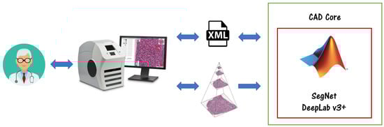
Figure 2.
CAD architecture. Physicians can visualize and annotate the WSIs using Aperio ImageScope software. The developed Deep Learning models can interact with ImageScope through an XML interface.
Table 2.
System Details.
3.2.2. Semantic Segmentation Workflow
To obtain an estimate of the Karpinski score, we must detect and classify all the glomeruli which appear in the WSI. We first use a semantic segmentation CNN to obtain a pixel-level classification, distinguishing between pixels which belongs to background, sclerotic and non-sclerotic glomeruli. Then, we must turn these pixel-level classifications into object detections, so that we can count the number of sclerotic and non-sclerotic glomeruli. The general schema for our semantic segmentation-based glomerular detector is depicted in Figure 3.
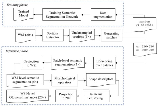
Figure 3.
Semantic Segmentation approach architecture. The top part describes how to train the CNN. The bottom part explains how to use the trained model for performing inference, and the related morphological and clustering post-processing steps.
The first step in our workflow consists of segmenting the sections present in the WSI. At this purpose, we used classical Image Processing techniques as thresholding, morphological operators, connected components labelling, and eventually, clustering. A similar preprocessing step has also been done by Ledbetter et al. [3]. We refer to the module performing this step as Sections Extractor. To reduce the very large dimension of WSIs, which can be overwhelming for Deep Learning algorithms, we undersampled the sections by a factor of 4. The original WSIs have a magnification of 20×, after undersampling it becomes equivalent to a magnification of 5×. This operation leads to an effective downsampling of the images from a resolution of about 8000 × 8000 pixels to a resolution of about 2000 × 2000 pixels. Since the section obtained this way was still too large to fit in our GPU, we divided it in patches. During training, we randomly sampled patches of size 656 × 656, with a mechanism to avoid to take too many patches only with negatives samples. The random patches sampled during the training process are then fed to a data augmentation block that performs different augmentations, as reported in Table 3. Augmentations are generated on-the-fly for each epoch within random ranges, so the network always processes slightly different input data, thus reducing the risk of overfitting. In the inference phase, we take patches of size 656 × 656 pixels, with an overlap between successive windows of 200 × 200 pixels. Please note that in semantic segmentation is important to have a larger context for performing inference, when the approach involves a sliding window processing [28]. After we get the predicted masks for glomeruli at patch-level, we project them to the original WSI, to get the WSI-level predicted mask. At this point, we apply morphological operators to remove noisy points and smooth the glomeruli shapes. We then analyze shape descriptors to understand if it is necessary to perform a clustering operation. In the end, the obtained mask is projected to 20× resolution, corresponding to oversampling by 4, using nearest-neighbour interpolation. Please note that in this work, all the resizing operations involving the digital pathology images are obtained using bicubic interpolation, while all the resizing operations involving the categorical masks are obtained using nearest-neighbour interpolation.
Table 3.
Augmentations.
3.2.3. Morphological Operators and Clustering
Adapting a semantic segmentation network to perform object detection poses some challenges. The task of semantic segmentation consists of labelling only individual pixels, which mainly captures textural information. In contrast to architectures explicitly tailored to Object Detection, such as Faster R-CNN [29] or Mask R-CNN [30], where there are anchor boxes, the network does not look for objects, it just tries to classify individual pixels. To extend the semantic segmentation model into an instance segmentation one, we must use different morphological operators and clustering algorithms as post-processing steps.
Morphological operators are applied only to binary masks obtained as the output of the semantic segmentation networks. First, we smooth the shapes of objects performing a morphological closing operation, with a disk of radius 5 pixels as structuring element, and with the morphological flood-fill operation. Then, we delete small objects and noisy points using opening operator, with a disk of radius 10 pixels as structuring element, and area opening operator, removing connected regions with an area below 1000 pixels. Examples are depicted in Figure 4, where binary masks are overlapped to the biopsy images for visualization purposes. Masks relative to non-sclerotic and sclerotic glomeruli are green and red colored, respectively. Lastly, we analyze the shape descriptors for each of these objects to understand if there are touching objects we need to cluster. The sequence of morphological operators used is depicted in Figure 5.
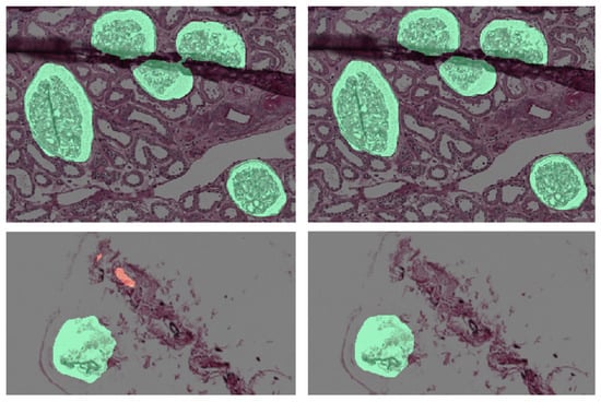
Figure 4.
(Left) Semantic Segmentation output. (Right) After Morphological Operators.
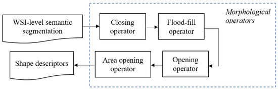
Figure 5.
Morphological operators sequence applied to the output masks from the semantic segmentation network. The output of the morphological post-processing is used for calculating shape descriptors to eventually perform clustering.
An important observation is that individual glomeruli have convex shapes, so their area is pretty similar to their convex area. We perform a K-means clustering based on the difference between the convex area and the area, as specified in Equation (1).
We decide the number K of clusters according to deltaArea: if deltaArea ≤ 900, ; if deltaArea > 900 and deltaArea ≤ 5000, ; if deltaArea > 5000, . The values of deltaArea and the corresponding K have been empirically determined on the trainval set. Confusion matrices reported later have been obtained after the clustering with the configuration based on deltaArea. Examples of glomeruli before clustering are depicted in Figure 6a,c. The corresponding images after clustering are shown in Figure 6b,d.
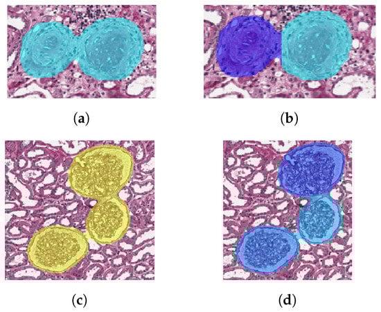
Figure 6.
Examples of K-means clustering for both sclerotic and non-sclerotic glomeruli. The number K of clusters is determined according to deltaArea defined in (1). (a) Sclerotic glomeruli before clustering. (b) Sclerotic glomeruli after clustering, with K = 2. (c) Non-sclerotic glomeruli before clustering. (d) Non-sclerotic glomeruli after clustering, with K = 3.
3.2.4. Data Augmentation
Tellez et al. analyzed the problem of stain color variation in digital pathology very deeply [31]. They proposed different solutions for both stain color augmentation and stain color normalization. In this work, we exploited techniques proposed by them such as morphological transformations and Hue-Saturation-Value (HSV) shifts. An interesting morphological transformation is the elastic deformation; it was originally proposed by Simard et al. [32] for the analysis of visual documents, and then has had a widespread application in medical imaging, as also shown by U-Net authors [28]. We used elastic deformation to generate plausible alterations of glomeruli shapes, increasing the variability of training images and thus reducing the risk of overfitting. An example of elastic deformation applied to our images is depicted in Figure 7. Examples of HSV shift are depicted in Figure 8.
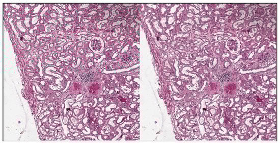
Figure 7.
Elastic deformation example. Left: original image. Right: after elastic deformation with , .
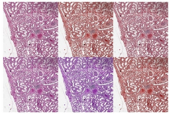
Figure 8.
HSV shift examples. Top Left: original image. Top Center: , . Top Right: , . Bottom Left: , . Bottom Center: , . Bottom Right: , .
A summary of the data augmentation techniques used for the training process is reported in Table 3. The augmentations in group 1 are independently performed, each with a given probability p. Resize augmentation used here is slightly different from standard resize; in fact, we apply mirroring padding (instead of zero padding) when we perform a resize which shrinks the image size. Augmentations, such as mirroring padding, which alter the morphology of the image are also executed for the mask. From the augmentations reported in group 2, only one is made. Group 3 contains only one augmentation, which is performed with a given probability. The augmentations are performed in the order they compare in the table, i.e., before the four in group 1, then one of group 2 and in the end the one of group 3.
3.2.5. Hyperparameters Tuning
We tried different semantic segmentation network architectures. For SegNet and DeepLab v3+ we tuned hyperparameters according to Table 4. Please note that DeepLab v3+ with ResNet-18 backbone is more lightweight than SegNet, and this allowed us to use a larger mini-batch size, with eight patches per mini-batch. With our GPU, SegNet was trained with only one patch per mini-batch. More details about hyperparameters can be found in MATLAB documentation [33].
Table 4.
Hyperparameters.
4. Experimental Results
We distinguish between the results obtained at pixel-level (semantic segmentation task) and at object detection level.
In particular, for the semantic segmentation task we group the metrics in Dataset Metrics and Class Metrics [33].
The group of Dataset Metrics includes semantic segmentation metrics aggregated over the data set: Global Accuracy, Mean Accuracy (the mean of the accuracies calculated per class), Mean IoU (the mean of the IoUs calculated per class), Weighted IoU (mean of the IoUs, weighted by the number of pixels in the class) and Mean F-score (mean of the F-measures calculated per class).
The group of Class Metrics includes semantic segmentation metrics calculated for each class, namely: Accuracy (2), IoU (3) and Mean F-score (F-measure for each class, averaged over all images).
For the object detection task, confusion matrices are calculated assuming that a true positive match between predicted mask and ground truth mask has pixel-wise IoU (3) of at least 0.2. Besides confusion matrices, the metrics used for assessing the results of the object detection task are:
The best results on non-sclerotic glomeruli have been obtained using DeepLab v3+, while for sclerotic glomeruli the best model was SegNet. An example of the output of our semantic segmentation framework is depicted in Figure 9.
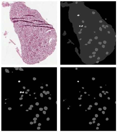
Figure 9.
Top Left: original image. Top Right: ground truth. Bottom Left: SegNet prediction. Bottom Right: DeepLab v3+ prediction. Sclerotic glomeruli and non-sclerotic ones are white and gray colored, respectively.
4.1. Pixel-Level Metrics
Pixel-level dataset metrics for both SegNet and DeepLab v3+ are reported in Table 5. The pixel-level class metrics of SegNet and DeepLab v3+ are reported in Table 6 and Table 7, respectively. The normalized pixel-level confusion matrix are in Table 8 and Table 9. Pixel-level confusion matrices are normalized per row; B, NS, S stand for Background, Non-sclerotic and sclerotic, respectively.
Table 5.
Dataset Metrics.
Table 6.
Class Metrics SegNet.
Table 7.
Class Metrics Deeplab v3+.
Table 8.
Normalized pixel-level Confusion Matrix SegNet.
Table 9.
Normalized pixel-level Confusion Matrix Deeplab v3+.
4.2. Object Detection Metrics
In object detection confusion matrices B, NS, S stand for Background, Non-sclerotic and Sclerotic, respectively.
The object detection confusion matrices for SegNet and DeepLab v3+ are reported in Table 10 and Table 11, respectively. The detection metrics for both the proposed models and a comparison with the method proposed by Marsh et al. [8] are reported in Table 12. The SegNet-based model obtained a better F-score for both the glomeruli classes. The DeepLab v3+-based model obtained a better F-score for non-sclerotic glomeruli and a slightly worse F-score for sclerotic glomeruli.
Table 10.
Object Detection Confusion Matrix SegNet.
Table 11.
Object Detection Confusion Matrix Deeplab v3+.
Table 12.
Performance Comparison for Detection Metrics.
5. Conclusions and Future Work
The proposed approach allowed us to obtain high performance both at pixel and object detection level. The semantic segmentation achieved mean F-score higher than 0.81 and Weighted IoU higher than 0.97 for both SegNet and Deeplab v3+ approaches; the glomeruli detection achieved 0.924 as best F-score for non-sclerotic glomeruli and 0.730 as best F-score for sclerotic glomeruli. We compared our obtained performance with the state of the art. As stated in the Section 1, there are three main works that face the problem of glomerular classification. Ginley et al. considered the glomerular assessment for patients affected by diabetic nephropathy but not for transplantation purposes [7]. Hermsen et al. considered many tissue classes, but the number of sclerotic glomeruli in their datasets is too small for a comparison with our method [14]. Marsh et al. considered the problem of global glomerulosclerosis from kidney transplant biopsies with haematoxylin and eosin (HE) stain [8]. The performance comparison between our proposed methods and Marsh et al. work is reported in Table 12. The obtained results show an improvement over the work of Marsh et al. Thus, CNNs for Semantic Segmentation are a viable approach for the purpose of glomerular segmentation and classification, allowing the obtaining of a reliable estimate of the global glomerulosclerosis. Assessing the suitability of kidney from ECD donors relies in many centers on the histological examination of kidney biopsies performed at the time of organ retrieval and processed and evaluated by on-call pathologist that, not necessarily, is an expert trained in renal pathology. The importance of training in renal pathology when assessing biopsy of such cases has been evaluated in some studies reporting better correlation with subsequent allograft outcome of histological scores provided by renal pathologists compared to those provided by general pathologist with potential risk of “overscoring” and the potential of discarding kidneys that could have been potentially transplanted [34,35,36]. The results were validated by the renal pathologists which assessed the reliability of the proposed workflow; the applied methodology constitutes a milestone in the creation of a CAD system for the renal transplant assessment. The proposed system could help pathologists in accomplishing the laborious task of evaluating the eligibility of a kidney for transplantation, providing a rapid and accurate result. Future work will include the use of Deep Learning models explicitly designed for the detection task, such as Faster R-CNN and Mask R-CNN.
Author Contributions
Conceptualization, N.A., G.D.C. and V.B.; Data curation, M.R., F.P. and L.G.; Methodology, N.A. and G.D.C.; Supervision, F.M., L.G. and V.B.; Validation, M.T.R., M.R., F.P. and L.G.; Writing—original draft, N.A.; Writing—review & editing, G.D.C., A.B., F.M., M.T.R., S.M., U.V., M.R., F.P., L.G. and V.B. All authors have read and agreed to the published version of the manuscript.
Funding
This work has been partially funded by the Italian Apulian Region project “SOS – Smart Operating Shelter” (INNONETWORK n. 9757YR7).
Conflicts of Interest
The authors declare no conflict of interest.
References
- Temerinac-Ott, M.; Forestier, G.; Schmitz, J.; Hermsen, M.; Bräsen, J.; Feuerhake, F.; Wemmert, C. Detection of glomeruli in renal pathology by mutual comparison of multiple staining modalities. In Proceedings of the IEEE 10th International Symposium on Image and Signal Processing and Analysis, Ljubljana, Slovenia, 18–20 Sepember 2017; pp. 19–24. [Google Scholar]
- Gallego, J.; Pedraza, A.; Lopez, S.; Steiner, G.; Gonzalez, L.; Laurinavicius, A.; Bueno, G. Glomerulus classification and detection based on convolutional neural networks. J. Imaging 2018, 4, 20. [Google Scholar] [CrossRef]
- Ledbetter, D.; Ho, L.; Lemley, K.V. Prediction of Kidney Function from Biopsy Images Using Convolutional Neural Networks; Los Alamos National Lab: Santa Fe, NM, USA, 2017; pp. 1–11.
- Gadermayr, M.; Dombrowski, A.K.; Klinkhammer, B.M.; Boor, P.; Merhof, D. CNN Cascades for Segmenting Whole Slide Images of the Kidney. arXiv 2017, arXiv:1708.00251. [Google Scholar]
- Cascarano, G.D.; Debitonto, F.S.; Lemma, R.; Brunetti, A.; Buongiorno, D.; De Feudis, I.; Guerriero, A.; Rossini, M.; Pesce, F.; Gesualdo, L.; et al. An Innovative Neural Network Framework for Glomerulus Classification Based on Morphological and Texture Features Evaluated in Histological Images of Kidney Biopsy; Springer: Berlin, Germany, 2019; pp. 727–738. [Google Scholar] [CrossRef]
- Kawazoe, Y.; Shimamoto, K.; Yamaguchi, R.; Shintani-Domoto, Y.; Uozaki, H.; Fukayama, M.; Ohe, K. Faster R-CNN-based glomerular detection in multistained human whole slide images. J. Imaging 2018, 4, 91. [Google Scholar] [CrossRef]
- Ginley, B.; Lutnick, B.; Jen, K.Y.; Fogo, A.B.; Jain, S.; Rosenberg, A.; Walavalkar, V.; Wilding, G.; Tomaszewski, J.E.; Yacoub, R.; et al. Computational Segmentation and Classification of Diabetic Glomerulosclerosis. J. Am. Soc. Nephrol. 2019, 30, 1953–1967. [Google Scholar] [CrossRef] [PubMed]
- Marsh, J.N.; Matlock, M.K.; Kudose, S.; Liu, T.C.; Stappenbeck, T.S.; Gaut, J.P.; Swamidass, S.J. Deep learning global glomerulosclerosis in transplant kidney frozen sections. IEEE Trans. Med. Imaging 2018, 37, 2718–2728. [Google Scholar] [CrossRef] [PubMed]
- Karpinski, J.; Lajoie, G.; Cattran, D.; Fenton, S.; Zaltzman, J.; Cardella, C.; Cole, E. Outcome of kidney transplantation from high-risk donors is determined by both structure and function. Transplantation 1999, 67, 1162–1167. [Google Scholar] [CrossRef]
- Remuzzi, G.; Grinyò, J.; Ruggenenti, P.; Beatini, M.; Cole, E.H.; Milford, E.L.; Brenner, B.M. Early experience with dual kidney transplantation in adults using expanded donor criteria. J. Am. Soc. Nephrol. 1999, 10, 2591–2598. [Google Scholar]
- Krizhevsky, A.; Sutskever, I.; Hinton, G.E. 2012 AlexNet. In Advances in Neural Information Processing Systems; MIT Press: Cambridge, MA, USA, 2012. [Google Scholar] [CrossRef]
- Dalal, N.; Triggs, B. Histograms of oriented gradients for human detection. In Proceedings of the IIEEE Computer Society Conference on Computer Vision and Pattern Recognition (CVPR’05), San Diego, CA, USA, 20–26 June 2005; Volume 1, pp. 886–893. [Google Scholar]
- Lindeberg, T. Detecting salient blob-like image structures and their scales with a scale-space primal sketch: A method for focus-of-attention. Int. J. Comput. Vis. 1993, 11, 283–318. [Google Scholar] [CrossRef]
- Hermsen, M.; de Bel, T.; Den Boer, M.; Steenbergen, E.J.; Kers, J.; Florquin, S.; Roelofs, J.J.; Stegall, M.D.; Alexander, M.P.; Smith, B.H.; et al. Deep Learning–Based Histopathologic Assessment of Kidney Tissue. J. Am. Soc. Nephrol. 2019, 30, 1968–1979. [Google Scholar] [CrossRef]
- Bevilacqua, V.; Pietroleonardo, N.; Triggiani, V.; Brunetti, A.; Di Palma, A.M.; Rossini, M.; Gesualdo, L. An innovative neural network framework to classify blood vessels and tubules based on Haralick features evaluated in histological images of kidney biopsy. Neurocomputing 2017, 228, 143–153. [Google Scholar] [CrossRef]
- Russakovsky, O.; Deng, J.; Su, H.; Krause, J.; Satheesh, S.; Ma, S.; Huang, Z.; Karpathy, A.; Khosla, A.; Bernstein, M.; et al. Imagenet large scale visual recognition challenge. Int. J. Comput. Vis. 2015, 115, 211–252. [Google Scholar] [CrossRef]
- Lecun, Y.; Bottou, L.; Bengio, Y.; Ha, P. LeNet. Proc. IEEE 1998. [Google Scholar] [CrossRef]
- Ma, Z.; Li, J.; Salemi, H.; Arnold, C.; Knudsen, B.S.; Gertych, A.; Ing, N. Semantic segmentation for prostate cancer grading by convolutional neural networks. In Proceedings of the SPIE Medical Imaging 2018: Digital Pathology, Houston, TX, USA, 10–15 February 2018; p. 46. [Google Scholar] [CrossRef]
- Tang, J.; Li, J.; Xu, X. Segnet-based gland segmentation from colon cancer histology images. In Proceedings of the IEEE 33rd Youth Academic Annual Conference of Chinese Association of Automation (YAC), Jiangsu, China, 18–20 May 2018; pp. 1078–1082. [Google Scholar]
- Alqazzaz, S.; Sun, X.; Yang, X.; Nokes, L. Automated brain tumor segmentation on multi-modal MR image using SegNet. Comput. Visual Media 2019, 5, 209–219. [Google Scholar] [CrossRef]
- Xiao, W.T.; Chang, L.J.; Liu, W.M. Semantic segmentation of colorectal polyps with DeepLab and LSTM networks. In Proceedings of the IEEE International Conference on Consumer Electronics-Taiwan (ICCE-TW), Taiwan, China, 19–21 May 2018; pp. 1–2. [Google Scholar]
- Tang, W.; Zou, D.; Yang, S.; Shi, J. DSL: Automatic liver segmentation with faster R-CNN and DeepLab. In Proceedings of the International Conference on Artificial Neural Networks, Rhodes, Greece, 4–7 October 2018; Springer: Berlin, Germany, 2018; pp. 137–147. [Google Scholar]
- Tang, W.; Zou, D.; Yang, S.; Shi, J.; Dan, J.; Song, G. A two-stage approach for automatic liver segmentation with Faster R-CNN and DeepLab. Neural Comput. Appl. 2020, 1–10. [Google Scholar] [CrossRef]
- Badrinarayanan, V.; Kendall, A.; Cipolla, R. SegNet: A Deep Convolutional Encoder-Decoder Architecture for Image Segmentation. IEEE Trans. Pattern Anal. Mach. Intell. 2017, 39, 2481–2495. [Google Scholar] [CrossRef] [PubMed]
- Chen, L.C.; Papandreou, G.; Kokkinos, I.; Murphy, K.; Yuille, A.L. DeepLab: Semantic Image Segmentation with Deep Convolutional Nets, Atrous Convolution, and Fully Connected CRFs. IEEE Trans. Pattern Anal. Mach. Intell. 2018, 40, 834–848. [Google Scholar] [CrossRef]
- Chen, L.C.; Zhu, Y.; Papandreou, G.; Schroff, F.; Adam, H. Encoder-decoder with atrous separable convolution for semantic image segmentation. In Lecture Notes in Computer Science (including subseries Lecture Notes in Artificial Intelligence and Lecture Notes in Bioinformatics); Springer: Berlin, Germany, 2018; Volume 11211 LNCS, pp. 833–851. [Google Scholar] [CrossRef]
- He, K.; Zhang, X.; Ren, S.; Sun, J. Deep residual learning for image recognition. In Proceedings of the IEEE Computer Society Conference on Computer Vision and Pattern Recognition, Las Vegas, NV, USA, 27–30 June 2016; pp. 770–778. [Google Scholar] [CrossRef]
- Ronneberger, O.; Fischer, P.; Brox, T. U-net: Convolutional networks for biomedical image segmentation. In Lecture Notes in Computer Science (Including Subseries Lecture Notes in Artificial Intelligence and Lecture Notes in Bioinformatics); Springer: Berlin, Germany, 2015; Volume 9351, pp. 234–241. [Google Scholar] [CrossRef]
- Ren, S.; He, K.; Girshick, R.; Sun, J. Faster R-CNN: Towards Real-Time Object Detection with Region Proposal Networks. IEEE Trans. Pattern Anal. Mach. Intell. 2017, 39, 1137–1149. [Google Scholar] [CrossRef]
- He, K.; Gkioxari, G.; Dollar, P.; Girshick, R. Mask R-CNN. In Proceedings of the IEEE International Conference on Computer Vision, Rio, Brazil, 14–21 October 2017. [Google Scholar] [CrossRef]
- Tellez, D.; Litjens, G.; Bándi, P.; Bulten, W.; Bokhorst, J.M.; Ciompi, F.; van der Laak, J. Quantifying the effects of data augmentation and stain color normalization in convolutional neural networks for computational pathology. Med. Image Anal. 2019, 58, 101544. [Google Scholar] [CrossRef]
- Simard, P.Y.; Steinkraus, D.; Platt, J.C. Best Practices for Convolutional Neural Networks Applied to Visual Document Analysis. In Proceedings of the ICDAR, Edinburgh, UK, 3–6 August 2003; Volume 3. [Google Scholar]
- MATLAB Documentation. Available online: https://www.mathworks.com/help/matlab/ (accessed on 19 November 2019).
- Azancot, M.A.; Moreso, F.; Salcedo, M.; Cantarell, C.; Perello, M.; Torres, I.B.; Montero, A.; Trilla, E.; Sellarés, J.; Morote, J.; et al. The reproducibility and predictive value on outcome of renal biopsies from expanded criteria donors. Kidney Int. 2014, 85, 1161–1168. [Google Scholar] [CrossRef]
- Haas, M. Donor kidney biopsies: Pathology matters, and so does the pathologist. Kidney Int. 2014, 85, 1016–1019. [Google Scholar] [CrossRef]
- Girolami, I.; Gambaro, G.; Ghimenton, C.; Beccari, S.; Caliò, A.; Brunelli, M.; Novelli, L.; Boggi, U.; Campani, D.; Zaza, G.; et al. Pre-implantation kidney biopsy: Value of the expertise in determining histological score and comparison with the whole organ on a series of discarded kidneys. J. Nephrol. 2020, 33, 167–176. [Google Scholar] [CrossRef] [PubMed]
© 2020 by the authors. Licensee MDPI, Basel, Switzerland. This article is an open access article distributed under the terms and conditions of the Creative Commons Attribution (CC BY) license (http://creativecommons.org/licenses/by/4.0/).