Modeling of Duty-Cycled MAC Protocols for Heterogeneous WSN with Priorities ^†

Abstract

Wireless Sensor Networks (WSN) have experienced an important revitalization, particularly with the arrival of Internet of Things applications. In a general sense, a WSN can be composed of different classes of nodes, having different characteristics or requirements (heterogeneity). Duty-cycling is a popular technique used in WSN, that allows nodes to sleep and wake up periodically in order to save energy. We believe that the modeling and performance evaluation of heterogeneous WSN with priorities operating in duty-cycling, being of capital importance for their correct design and successful deployment, have not been sufficiently explored. The present work presents a performance evaluation study of a WSN with these features. For a scenario with two classes of nodes composing the network, each with a different channel access priority, an approximate analytical model is developed with a pair of two-dimensional discrete-time Markov chains. Note that the same modeling approach can be used to analyze networks with a larger number of classes. Performance parameters such as average packet delay, throughput and average energy consumption are obtained. Analytical results are validated by simulation, showing accurate results. Furthermore, a new procedure to determine the energy consumption of nodes is proposed that significantly improves the accuracy of previous proposals. We provide quantitative evidence showing that the energy consumption accuracy improvement can be up to two orders of magnitude.

1. Introduction

A Wireless Sensor Network (WSN) is a collection of nodes, considered energy-constrained devices as they are powered by batteries, that cooperatively perform data collection, processing and communication activities. Some areas of application for WSN are in medical, industrial, agricultural and environmental monitoring. The technological evolution of sensors promise to facilitate the integration of WSN with the Internet of Things (IoT) and, therefore, improve applications such as the distribution of intelligent services (smart grid, smart water), intelligent transport systems (ITS) and smart homes [1,2,3,4,5]. However, efficient energy deployment is a crucial issue in WSN. Among the operations performed by nodes, the medium access coordinated by the Medium Access Control (MAC) protocol, and the consequent data transmission, consume a significant amount of energy [6,7].

Some recent WSN MAC protocol developments employ duty-cycling (DC) to save energy and maximize the WSN lifetime. In WSN MAC protocols operating with DC, idle nodes stay in the sleep mode in order to save energy. Nodes wake up only during packet exchange periods. Medium access in WSN is based on contention deploying a Carrier Sense Multiple Access and Collision Avoidance (CSMA/CA) mechanism, and the Request-to-send/Clear-to-send/DATA/Acknowledgment (RTS/CTS/DATA/ACK) handshake [8,9]. S-MAC (Sensor-MAC) was the first WSN MAC protocol that implemented DC and remains one of the most popular [10].

A certain degree of heterogeneity is typically present in many WSN [11,12,13,14,15]. A common modeling approach for heterogeneous WSN is to define different classes of nodes, and with different traffic patterns [16]. In our study, in addition, different node classes have different channel access priorities. For example, WSN deployments in emergency scenarios, such as fires, earthquakes or some medical applications, require that nodes send data towards a control center as soon as events occur. Therefore, nodes sending emergency data need to have medium access priority over other network nodes.

The modeling and performance evaluation of heterogeneous WSN with priorities operating in DC, being of capital importance for their correct design and successful deployment, have not been sufficiently explored. Most MAC protocols that deploy CSMA/CA are analytically modeled using Markov chains. Models in [17,18] are based on a discrete-time Markov chain (DTMC), allowing the characterization of the evolution of the state of the network along time. These models are relatively simple and accurate enough, but they cannot be directly applied to the performance evaluation of synchronous MAC protocols that use DC.

In [19,20,21,22], we found recent examples of the application of DTMC to the modeling and performance evaluation of homogeneous WSN scenarios operating in DC without priorities. The models proposed in [19,20] assume that the state of nodes is mutually independent, even though there is a certain degree of dependency between them in practice [21]. All these models were designed considering homogeneous scenarios, where nodes behave in the same way in terms of load. Therefore, these models do not consider the possibility of different loads or different channel access priorities.

Markov-based models for heterogeneous scenarios were presented in [23,24]. In [23], different classes of nodes are considered, including the assignment of different packet arrival rates for each class, but all nodes have the same access priority. In [24], priority schemes, including different classes of nodes, are considered but without the possibility of different arrival rates or different number of nodes per class. Although these models evaluate heterogeneous scenarios for WSN, they cannot be directly applied to WSN using a DC mechanism.

In [25], a preliminary performance evaluation model for WSN operating in DC that supports multiple classes of nodes was presented. For each class, the model allows to independently configure access priority, number of nodes per class, and packet arrival rate to nodes of the class (load). For clarity, we will refer to the MAC protocol proposed in [25] as Priority Sink Access MAC (PSA-MAC).

Previous schemes for energy consumption computation were based on procedures that did not fully exploit the system stationary distribution. Different intermediate terms were defined that lead to a less intuitive, less systematic, and less accurate procedure for energy consumption computation. See, for example, [19,20,21,22,25]. However, in this paper, we propose a novel computation method that is simple and accurate, as discussed later.

There are two main contributions of this paper. First, the analytical modeling and performance evaluation of a WSN where nodes deploy a MAC protocol that uses CSMA/CA, a DC mechanism such as the one used in PSA-MAC, and support different loads and access priorities. For a scenario with two classes of nodes composing the network, each with a different access priority, an approximate analytical model is developed with a pair of two-dimensional DTMC (2D-DTMC). Note that the same modeling approach can be used to analyze networks with a larger number of classes, as described in Section 3.3. This model extends the capability of the models presented in [21] in order to allow the modeling of different classes of nodes with different access priority assignments in heterogeneous network scenarios.

Second, the proposal of a new method to determine the energy consumption of a node that is more intuitive and systematic than those considered before. In addition, this method substantially outperforms previous ones in terms of accuracy when results are compared with those obtained by simulation.

The rest of the article is organized as follows. In Section 2, the network scenario is presented, and the model assumptions are defined. The mathematical model of the system is presented in Section 3. The analysis to determine the performance parameters is developed in Section 4. The results and their discussion is presented in Section 5. Finally, the conclusions are presented in Section 6.

2. Network Scenario

2.1. PSA-MAC Protocol

As in most MAC protocols operating in DC, in PSA-MAC, the time is divided into cycles of equal duration T, and each cycle consists of an active and sleep period, as in Figure 1. The active period is subdivided in two parts: the sync period of fixed duration $T_{sync}$, where SYNC packets are exchanged; and the data period, where DATA packets are exchanged.

During a sync period, nodes choose a sleep–awake schedule and exchange it with their neighbors using SYNC packets. These packets include the transmitter node address and the start time of their next active period. With this information, nodes coordinate to wake up simultaneously at the beginning of each sync period. SYNC and DATA packets are transmitted using the CSMA/CA contention mechanism in order to access the channel. In CSMA/CA active nodes generate a random backoff time and perform a channel carrier sensing procedure. A node is considered active when it has packets to transmit. If the channel is idle when the backoff timer expires, then nodes transmit a packet using the RTS/CTS/DATA/ACK handshake. When a winning node receives a CTS in response to its previous RTS, it transmits the SYNC or DATA packet and waits for the ACK.

During the data period, nodes transmit DATA packets. Active nodes generate a new backoff time at each data period initiation and perform carrier sensing before accessing the channel. In PSA-MAC, during the data period a node goes to sleep mode until the beginning of the next sync or data period when: (i) it loses the contention (hears a busy medium before its backoff time expires); (ii) it encounters a RTS collision; (iii) after a successful transmission (only one packet per cycle is transmitted).

2.2. Network Operation and Assumptions

We consider a heterogeneous WSN with N nodes of different classes, where all nodes listen to each other and send packets to a common sink node, as, for example, in Figure 2.

The scenario consists of a single cell cluster, but multiple clusters together may configure a larger network. In this work, the scenario of a single cluster is studied. Two classes of nodes are considered, and we assume that class 1 nodes have medium access priority over class 2 nodes. Other assumptions considered in this study are: (i) the sink node only receives packets, never transmits; (ii) for realistic scenarios, it has been shown that one or two retransmissions are enough to transmit a packet successfully [21]. Then, for simplicity, we consider an infinite retransmissions model, as a simpler modeling alternative to the more complex model of finite retransmissions; (iii) from the MAC perspective, the channel is ideal (error-free); (iv) packets arrive to the buffer (queue) of a node following a renewal process, and the number of packets that arrive in each cycle is characterized by independent and identically distributed random variables.

In the evaluated scenario, as expected, the sink responds to each received data packet with the corresponding CTS and ACK. In some scenarios, the sink might also send data to nodes, either configuration or data packets. However, in most applications, the desired information is typically collected by the sensor nodes and aggregated at the sink before being forwarded upstream. For example, health monitoring applications [26]. As the load of configuration traffic, if present, should be typically small and sporadic, we have not included it in the model. Nevertheless, sink traffic can be included in the network, associating it to one or both of the two considered classes. For scenarios where the traffic offered by the sink to the nodes of a class is similar to the one offered by the rest of nodes of the same class (homogeneous load case), please refer to [21]. There, a single class is considered, the sink is considered as another class member node, and all class member nodes exchange packets among themselves.

The modeling approach can also be extended to scenarios with a non-ideal channel. For example, in [27], a DTMC model is proposed to investigate the impact of channel impairments on the performance of a single class WSN with no priorities, where the packet error probability depends on the packet length. The model in [27] can be readily adapted to a scenario with priorities as the one studied in this paper. Please refer to Section 3.3 for further details.

Each node has a finite buffer with a storage capacity of Q packets that are served according to a FIFO discipline. For simplicity, we assume that the number of packets arriving to a buffer per cycle follows a discrete Poisson distribution of mean $\lambda T$, where $\lambda$ is the packet arrival rate, and T is the cycle duration. However, the proposed analytical model is generic enough to support any other distribution. For class 1 nodes, the nodes with the highest channel access priority, we consider low traffic loads, since in realistic application, for instance, emergencies, the high priority information to transmit is small and sporadic. Nerveless, the proposed model supports any load for class 1 nodes.

2.3. Assignment of Medium Access Priorities

A way to prioritize the medium access for class 1 nodes over the class 2 nodes is to assure that class 1 devices complete the medium access procedure before class 2 devices. Figure 3 shows the medium access procedure for both classes along time, where the sync period for both classes of nodes has been omitted.

In the proposed WSN operation, the medium access priority is granted to class 1 nodes by following the next access procedure. At the beginning of a cycle, only active class 1 nodes trigger the medium access and contend for medium access among themselves. Active class 2 nodes wake up just after the class 1 contention window ($W_1$) has ended, and if they detect an idle medium, they will proceed to transmit, activating their own contention mechanism. If class 2 nodes detect the medium occupied at that instant, they return to sleep mode and wake up again at the next cycle. We assume that the duration of a packet transmitted by a class 1 node is longer than $W_1$.

3. System Model

The expressions developed in Section 3 and Section 4 are equally applicable to both classes of nodes. We use a generic notation to define the model parameters associated with any of the two node classes, unless otherwise specified. For description convenience, one node of each class is selected arbitrarily as reference node, $R{N}_1$ and $R{N}_2$.

3.1. Access to the Medium

Active nodes generate random backoff times selected from the interval $\left[0,W-1\right]$. When the RN is active, it transmits a packet successfully if the other contending nodes choose backoff times larger than the one chosen by the RN. The packet transmitted by the RN will collide (fail) when the RN and one or more of the other contending nodes choose the same backoff time, and this backoff time is the smallest of those generated in the current cycle. If the backoff time generated by the RN is not the smallest one, two outcomes are possible: (i) another node is able to transmit successfully; (ii) other nodes will collide when transmitting. Nodes that lose the contention (because they hear a busy medium before their backoff time expires), or find an RTS packet collision, go to sleep mode and remain in that mode until the active period of the next cycle.

For notation simplicity, N denotes the number of nodes of a given class. Considering a cycle where the RN is active, k denotes the number of nodes that are also active in the same cycle, besides the RN, $0\le k\le K=N-1$.

Let $P_{s,k}$, $P_{sf,k}$ and $P_{f,k}$, be the probabilities that the RN transmits a packet successfully, transmits a packet (successfully or with collision), and transmits with failure (collision), respectively, when the RN contends with other k nodes. Then,

$$\begin{array}{ccc}\hfill P_{s,k}& =& \sum _{i=0}^{W-1}\frac{1}{W}{\left(\frac{W-1-i}{W}\right)}^k,\hfill \end{array}$$

(1)

$$\begin{array}{ccc}\hfill P_{sf,k}& =& \sum _{i=0}^{W-1}\frac{1}{W}{\left(\frac{W-i}{W}\right)}^k,\hfill \end{array}$$

(2)

$$\begin{array}{ccc}\hfill P_{f,k}& =& P_{sf,k}-P_{s,k}=\frac{1}{W}.\hfill \end{array}$$

(3)

Note that $P_{s,k}$ is the probability that the RN chooses a backoff value from the interval $\left[0,W-1\right]$, and the other k nodes choose a larger value. Probabilities $P_{sf,k}$ and $P_{f,k}$ can be described in similar terms.

Conditioned on a successful or unsuccessful packet transmission by the RN, when contending with other k nodes, the average backoff times are given by,

$$\begin{array}{ccc}\hfill B{T}_{s,k}& =& \frac{1}{P_{s,k}}\sum _{i=0}^{W-1}i·\frac{1}{W}{\left(\frac{W-1-i}{W}\right)}^k,\hfill \end{array}$$

(4)

$$\begin{array}{ccc}\hfill B{T}_{f,k}& =& \sum _{i=0}^{W-1}i·\left[{\left(\frac{W-i}{W}\right)}^k-{\left(\frac{W-1-i}{W}\right)}^k\right].\hfill \end{array}$$

(5)

3.2. System with Two Classes and Priorities

In this subsection, we model the time evolution of the number of packets in the queue of $R{N}_1$ and $R{N}_2$, and the number of active nodes in the network, by a pair of 2D-DTMC, one chain for each node class. The state of each node class is represented by the tuple $(i,m)$, where i, $i\le Q$, is the number of packets in the queue of the RN, and m, $m\le K=N-1$, is the number of active nodes of the corresponding class other than the RN.

Let $P_{(i,m),(j,n)}$ be the transition probability from state $(i,m)$ to state $(j,n)$. The first 2D-DTMC is adapted from [21], and is proposed to describe the time evolution of the state of class 1 nodes. The second 2D-DTMC is taken from [25] and is proposed to describe the time evolution of the state of class 2 nodes. For clarity and paper length limitations, the transition probabilities of both 2D-DTMC are presented in detail in [28].

Note that the representation of the network state is an approximation. For each class, the state of the set of nodes other than the RN is approximated using only the m parameter [21,22]. As it will be justified later, this approximation provides very accurate results.

3.3. Solution of the Pair of 2D-DTMC

The solution of each of these 2D-DTMC can be obtained by solving the following system of linear equations,

$$\begin{array}{c}\hfill \mathit{\pi }\mathit{P}=\mathit{\pi },\mathit{\pi }\mathit{e}=1,\end{array}$$

(6)

where $\mathit{\pi }=\left[\pi \right(i,k\left)\right]$ is the stationary distribution, P is the transition probability matrix, the elements of which are defined in [28] (the referred technical report includes two tables: Table 1 for class 1 nodes, and Table 2 for class 2 nodes), and e is a column vector of ones.

The probability $P_s$ that the RN transmits a packet successfully in a random cycle, conditioned on the RN being active in that cycle, is given by,

$$\begin{array}{ccc}\hfill P_s& =& \frac{1}{G}\sum _{i=1}^Q\sum _{k=0}^K\pi (i,k)·P_{s,k},\hfill \end{array}$$

(7)

$$\begin{array}{ccc}\hfill G& =& \sum _{i=1}^Q\sum _{k=0}^K\pi (i,k)=1-\sum _{k=0}^K\pi (0,k).\hfill \end{array}$$

(8)

As observed in [28], to determine the stationary distribution, $P_s$ is required, i.e., the stationary distribution is a function of $P_s$, $\mathit{\pi }\left(P_s\right)$. By solving the set of Equation (6), $\mathit{\pi }\left(P_s\right)$ can be determined for a given $P_s$. Then, a new $P_s$ can be obtained from Equation (7). We follow a fixed-point iteration procedure and denote its solution by $\mathit{\pi }$.

To determine the solution of the second 2D-DTMC, the solution of the first 2D-DTMC is required. In particular, one of the parameters of the second 2D-DTMC is the fraction of time (cycles) that the channel remains idle due to the inactivity of the high priority nodes (class 1 nodes), $R_{1,0}={\pi }_1(0,0)$, where ${\pi }_{\mathbf{1}}$ is the stationary distribution of the first 2D-DTMC.

For a system with a larger number of priorities, the solution of the stationary distribution of any priority class would previously require the solution of stationary distributions of all higher priority classes. Please refer to [28] for additional details.

4. Performance Parameters

In this section, we define different expressions to determine the throughput, average packet delay and average energy consumption per cycle. The following expressions are applicable to both classes of nodes.

4.1. Throughput

The node throughput $\eta$ is defined as the average number of packets successfully transmitted by a node in a cycle, and it is determined by,

$$\begin{array}{ccc}\hfill \eta & =& \sum _{i=1}^Q\sum _{k=0}^K\pi (i,k)·P_{s,k}.\hfill \end{array}$$

(9)

In a network of N nodes, the aggregated throughput, $Th$, expressed in packets per cycle is obtained as,

$$\begin{array}{c}\hfill Th=N·\eta .\end{array}$$

(10)

4.2. Average Packet Delay

Let D be the average delay (in cycles) that a packet experiences from its arrival until its successful transmission. Then, D can be determined by applying Little’s law,

$$\begin{array}{ccc}\hfill D& =& \frac{N_{av}}{\eta },\hfill \end{array}$$

(11)

$$\begin{array}{ccc}\hfill N_{av}& =& \sum _{i=0}^{Q}i{\pi }_i,\hfill \end{array}$$

(12)

$$\begin{array}{ccc}\hfill {\pi }_i& =& \sum _{k=0}^K\pi (i,k).\hfill \end{array}$$

(13)

Note that ${\pi }_i$ is the stationary probability of finding i packets in the queue of the RN, and $N_{av}$ is the average number of packets in the RN queue.

4.3. New Improved Method to Determine the Average Energy Consumption

As observed in Figure 1, the active period of a cycle is subdivided into sync and data periods. The energy consumed during the active period represents the most significant contribution to the total energy consumption. In this section, we compute the average energy consumed by the RN in the data period. Note that only the energy consumed by the radio frequency transceiver is considered. The energy consumed by sensor nodes due to events related to specific sensing tasks is dependent on the specific application. Then, as it does not depend on the MAC, it is not included in this study.

Let $E_s^{tx}$, $E_f^{tx}$ and $E_{oh}$, be the average energy consumption per cycle terms, when the RN transmits successfully, it transmits with failure (collision), and when it overhears other node transmissions, respectively. Then, the average energy consumed by the RN per cycle is given by,

$$\begin{array}{c}\hfill E_d=E_s^{tx}+E_f^{tx}+E_{oh}.\end{array}$$

(14)

$E_s^{tx}$ is obtained as,

$$\begin{array}{ccc}\hfill E_s^{tx}& =& \sum _{i=1}^Q\sum _{k=0}^K\pi (i,k)P_{s,k}(P_{s,1}^{tx}+P_{s,2}^{tx}+P_s^{rx}+B{T}_{s,k}{P}_{rx}),\hfill \end{array}$$

(15)

$$\begin{array}{ccc}\hfill P_{s,1}^{tx}& =& t_{RTS}{P}_{tx},P_{s,2}^{tx}=t_{DATA}{P}_{tx},\hfill \end{array}$$

(16)

$$\begin{array}{ccc}\hfill P_s^{rx}& =& \left[t_{CTS}+t_{ACK}+4D_p\right]P_{rx}.\hfill \end{array}$$

(17)

where $t_{RTS}$, $t_{DATA}$, $t_{CTS}$ and $t_{ACK}$, are the transmission times for the RTS, DATA, CTS and ACK packets, respectively. $P_{tx}$ and $P_{rx}$ are the transmission and reception power levels, and $D_p$ is the one-way propagation delay. The term $E_f^{tx}$ is determined by,

$$\begin{array}{ccc}\hfill E_f^{tx}& =& \sum _{i=1}^Q\sum _{k=0}^K\pi (i,k)P_{f,k}(P_f^{tx}+B{T}_{f,k}{P}_{rx}+P_f^{rx}),\hfill \end{array}$$

(18)

$$\begin{array}{ccc}\hfill P_f^{tx}& =& t_{RTS}{P}_{tx},P_f^{rx}=2D_p{P}_{rx},\hfill \end{array}$$

(19)

Finally, $E_{oh}$ is obtained by,

$$\begin{array}{ccc}\hfill E_{oh}& =& \sum _{i=1}^Q\sum _{k=0}^K\pi (i,k)[k{P}_{s,k}\left(B{T}_{s,k}{P}_{rx}\right)+{\widehat{P}}_{f,k}\left(B{T}_{f,k}{P}_{rx}\right)],\hfill \end{array}$$

(20)

$$\begin{array}{ccc}\hfill {\widehat{P}}_{f,k}& =& \sum _{i=1}^W\left[\sum _{n=2}^k\left(\genfrac{}{}{0pt}{}{k}{n}\right){\left(\frac{1}{W}\right)}^n{\left(\frac{W-i}{W}\right)}^{k-n+1}\right].\hfill \end{array}$$

(21)

where ${\widehat{P}}_{f,k}$ is the probability that two or more of the other k nodes differ from the RN chosen with the smallest backoff value and, therefore, smaller than the backoff value chosen by the RN. In this case, the RN will lose the contention, and the other two or more k nodes will transmit with collision.

In summary, an active RN overhears the channel when: (i) one of the other k nodes transmits successfully (with probability $k{P}_{s,k}$); or (ii) two or more of the other k nodes collide (with probability ${\widehat{P}}_{f,k}$). Note that if the RN is not active, it will not listen to the channel, as we assume that the sink only receives and never transmits.

For class 2 nodes, the same expressions are applied to obtain the energy consumed during the active period $E_{d2}$. However, an additional term must be added to account for the energy consumed by class 2 nodes to sense the channel when they wake up but they sense a busy channel. We denote this term as $E_0=ts·P_{rx}$, where $ts$ is the duration of one time slot.

Let $E_1$ and $E_2$ be the average energy consumed by class 1 and class 2 nodes per cycle, respectively. The final expressions to determine the energy consumption for both classes of nodes are given by,

$$\begin{array}{ccc}\hfill E_1& =& E_{d1},\hfill \end{array}$$

(22)

$$\begin{array}{ccc}\hfill E_2& =& (1-R_{1,0})E_0+R_{1,0}·E_{d2}.\hfill \end{array}$$

(23)

where $R_{1,0}$ is the stationary probability of finding no active class 1 nodes in a cycle (fraction of cycles where all class 1 nodes are inactive). As $E_0\approx 0$, we approximate $E_2\approx R_{1,0}·E_{d2}$.

The proposed model to determine the energy consumed by a node allows to accurately predict the lifetime of a node of any priority class in the network. When nodes start operating with different battery levels, as nodes deplete their batteries, they can be removed from the network, and then a new stationary distribution must be computed.

Performance Evaluation of the Improved Method to Determine Energy Consumption

The new procedure to determine the energy consumed by a node per cycle was described in Section 4.3. In this subsection, we highlight its advantage in terms of accuracy improvement, particularly for class 2 nodes, with respect to the energy consumption computation method proposed in [19,20,21,22,25].

As a summary, we will say that previous procedures required the computation of additional intermediate terms (see Section IV.C, from [25]), in addition to the stationary distribution $\pi (i,k)$. However, the new procedure described by Equations (14)–(20), only requires $\pi (i,k)$.

As an example,

Table 1. Relative errors for the two energy computation methods.

Class 2
Scenario 1			Scenario 2
${\lambda }_2=2.5$	Old	New	${\lambda }_2=1.5$	Old	New
	3.851 %	0.569 %		4.953 %	0.036 %

shows the relative error of the energy consumption of class 2 nodes computed into two specific scenarios defined in Section 5. To highlight the difference with the previous computation method in [25], we have chosen two operating points where the worst accuracy is obtained. Note that relative values are obtained as $|x-y|/y$, where x is the value obtained by the corresponding analytical computation procedure, and y is the value obtained by simulation.

As shown, on average, the new computation method considerably outperforms the previous one, by up to two orders of magnitude. In addition, it is more systematic and intuitive than the previous one, as it uses the stationary probability distribution more efficiently in the computation process.

5. Numerical Results

5.1. 2D-DTMC Model Validation

Results obtained from the proposed 2D-DTMC analytical model are validated by simulation. We have developed a discrete event simulator in C language that implements the physical transmission scheme and describes the time evolution of the sensor network state. At each cycle, each sensor receives packets according to a given discrete distribution. If a sensor has packets in its buffer, it contends with other nodes for channel access, and if it wins, it then transmits a DATA packet according to the described transmission scheme.

Simulation results are completely independent of those obtained by the analytical model. That is, the computation of the performance metrics by simulation does not use the system state representation, nor its stationary distribution, nor the mathematical expressions developed for the analytical model. The simulation results presented later are average values of measurements carried out along ${10}^8$ cycles. We have obtained confidence intervals with a 95% confidence level. However, as they are very small, for clarity they have been mostly omitted. For illustration purposes and as examples, confidence intervals are drawn for the top curves of Figure 4 and Figures 7–9.

In the following subsections, we show performance results obtained by the analytical model and by simulation. Simulation results are represented with red confidence intervals or red markers. Analytical results are represented with lines, or lines and markers. In many cases, the markers of analytical and simulation results totally overlap, and they are difficult to distinguish. In particular, red markers (simulation results) overlap and hide markers depicted with other colors (analytical results), which are the ones shown in the legends of the corresponding figures. As an example, in Figure 4, the average delay of the successfully transmitted packets is shown for both classes of nodes. Clearly, analytical and simulation results perfectly match, confirming that the analytical model is very accurate.

5.2. Scenarios and Parameter Configuration

In this section, the performance of a WSN, such as the one illustrated in Figure 2, is evaluated. We have considered two classes of nodes (1 and 2), with $N_1$ and $N_2$ populations. We have studied two scenarios (SC1 and SC2) with different configurations for each class of nodes, in terms of load and population. Configuration parameters are summarized in

Table 2. Parameter configuration.

Cycle duration (T)	60 $\mathbf{m}$s	Propagation Delay (${\mathit{D}}_{\mathit{p}}$)	0.1 $\mathsf{\mu }$s
$t_{SYNC}$, $t_{RTS}$, $t_{CTS}$ and $t_{ACK}$	0.18 $\mathrm{m}$s	Slot time ($ts$)	0.1 $\mathrm{m}$s
$t_{DATA}$	1.716 $\mathrm{m}$s	Contention window (W)	128 slots
DATA packet size	50 bytes	Buffer size (Q)	5 packets
Transmission power ($P_{tx}$)	52 $\mathrm{m}$W	Reception power ($P_{rx}$)	59 $\mathrm{m}$W
Number of nodes		Arrival packet rate (packets/s)
$N_1=5$ (SC1 and SC2)		${\lambda }_1=\{0.5,1.0\}$
$N_2=3N_1=15$ (SC1), $N_2=4N_1=20$ (SC2)		${\lambda }_2=\left[0.5,4.5\right]$

[29]. The performance parameters of interest are: average packet delay, throughput and average energy consumption.

For simplicity, in the evaluation scenario defined in this section, we have considered that nodes have sufficient energy so that the stationary regime is achieved before the battery of any node is depleted. When appropriately configured, the stationary regime is achieved after a small number of cycles. When nodes do not have the same initial energy, nodes that deplete their batteries stop operating, and, for modeling purposes, can be removed from the network. The proposed energy consumption procedure allows to predict with excellent accuracy the lifetime of a node with a given initial energy. Once the population of nodes of each class is readjusted, the model can be solved again until the next node stops operating.

5.3. Average Packet Delay

Figure 4 shows the average packet delay expressed in cycles, for both classes of nodes in SC1, and for two packet arrival rates for class 1 nodes (${\lambda }_1$).

We denote by $D_1$ and $D_2$ the average delay of packets transmitted successfully by nodes of class 1 and class 2, respectively. Observe in Figure 4 that $D_1$ is constant for the load range studied, as class 1 packets have access priority, and ${\lambda }_1$ and $N_1$ are both constant. In addition, it takes a very low value as we study realistic scenarios where class 1 nodes generate a small and sporadic load.

However, for nodes of class 2, the packet arrival rate takes values in the range ${\lambda }_2\in \left[0.5,4.5\right]$. Note that the fraction of class 2 packets that collide increases with ${\lambda }_2$. As the number of retransmissions increase, $D_2$ also increases. Note also that as class 1 traffic load increases, class 2 nodes perceive the channel as busy for longer periods. Therefore, class 2 nodes take longer to transmit their packets, and their delay increases.

Note that $D_1$ does not increase when ${\lambda }_1$ increases from 0.5 to 1 packets/s, as for both load values, the queues of class 1 nodes remain almost empty most of the time, i.e., nodes remain idle and access the channel rarely. Then, when a packet arrives, it is transmitted immediately, without neither delay nor collision.

Figure 5 shows the evolution of the average delay for class 2 nodes with ${\lambda }_1$ in both scenarios, and with different ${\lambda }_1$ values. Note that for SC1, $N_2=3N_1$, and for SC2, $N_2=4N_1$. Curves show that $D_2$ increases rapidly with ${\lambda }_2$, until approximately ${\lambda }_2=1$. For higher loads, $D_2$ increases slowly. As expected in SC2, where the number of nodes is larger, $D_2$ takes values higher than in SC1. When the number of nodes increases, contention also increases, and it takes longer to access the channel. Therefore, packets wait longer in the queue before being transmitted. In addition, more collisions and, hence, more retransmissions occur. Observe also that $D_2$ increases with ${\lambda }_1$. This can be explained in the same terms as those used to explain the results of Figure 4.

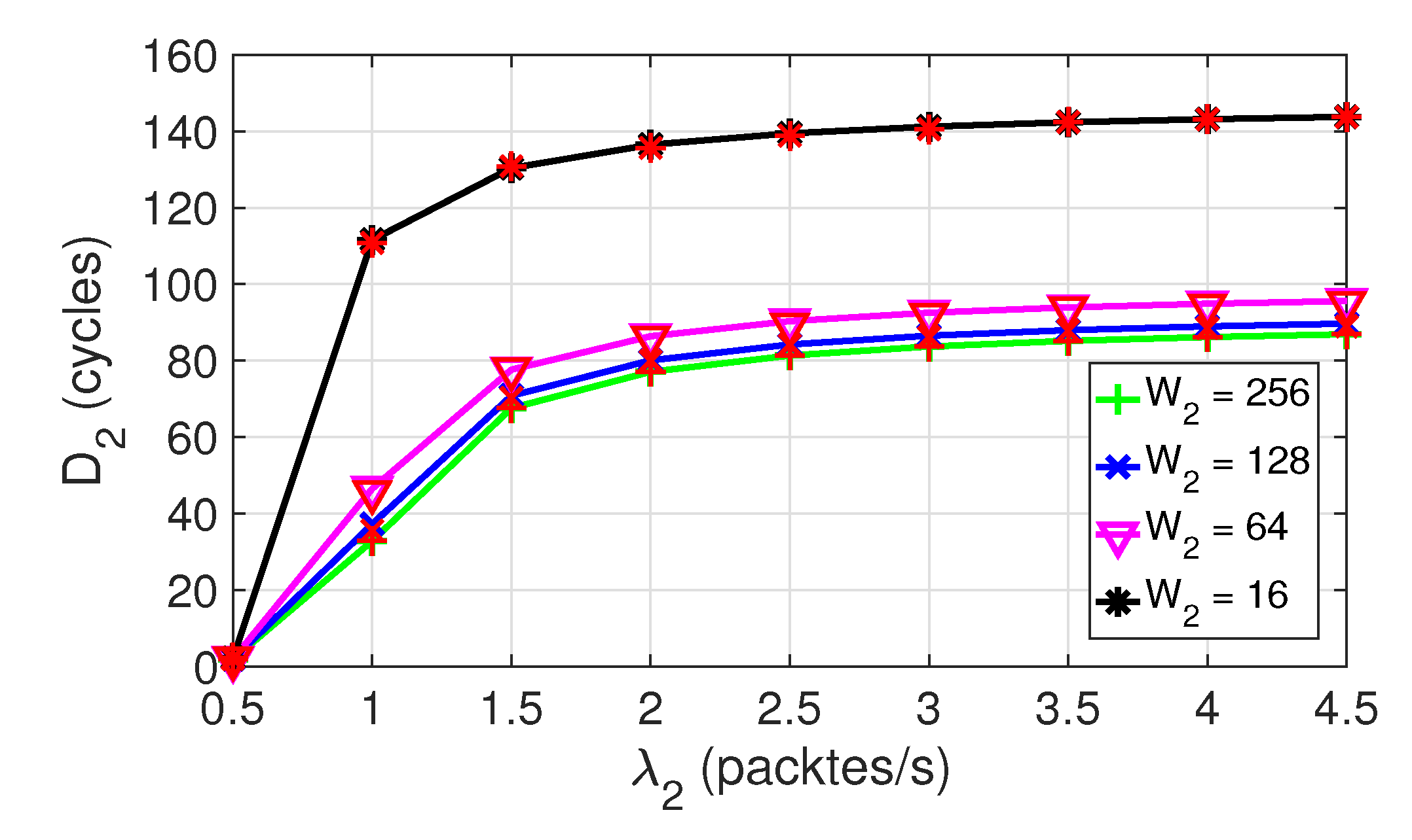
Figure 6 shows the evolution of the average delay for class 2 nodes with ${\lambda }_2$ with different contention window sizes $W_2$ in SC1. Results for Figure 6 (and Figure 10, shown later) have been obtained with the following configuration changes: $W_1=16$ and $W_2=\{16,64,128,256\}$. Note that in our model, the priority assignment is not affected by the contention window size, as explained in Section 2.3. The changes for $W_1$ and $W_2$ do not modify the defined priority but influence the delay. $W_1=16$ has been chosen because being $N_1$ small, the collision probability does not significantly change for the larger $W_1$ values. Recall that the collision probability was defined in Equation (3). In addition, it has been observed that $D_1$ does not significantly change when $W_1>16$.

However, for class 2 nodes, there is a significant impact when the value of $W_2$ changes. The probability that two or more backoff timer values for class 2 nodes coincide increases as $W_2$ decreases. Figure 6 clearly shows the effect of $W_2$ in $D_2$. For a fixed load, when $W_2$ increases, the probability of collision decreases and, therefore, $D_2$ decreases.

5.4. Throughput

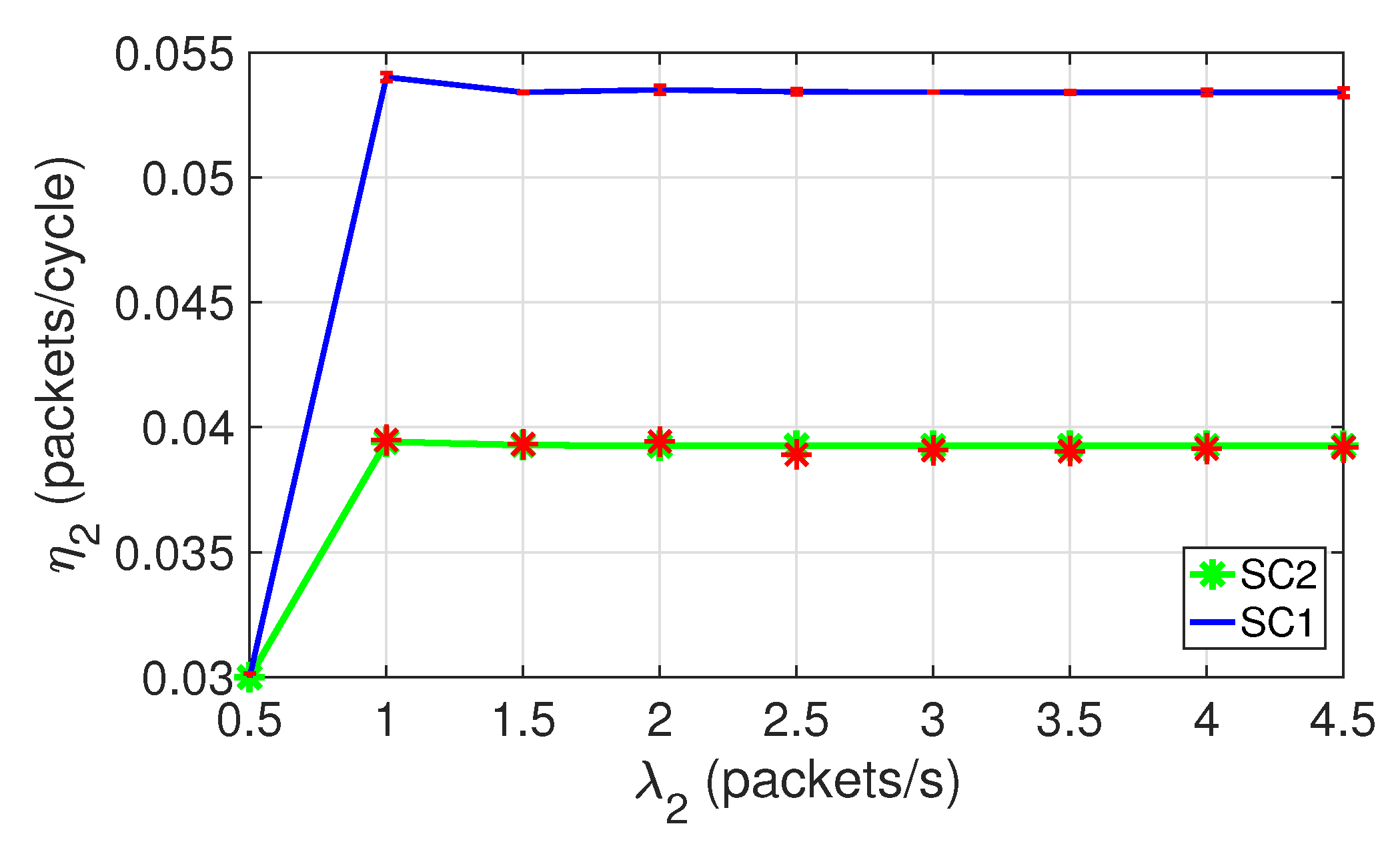
Figure 7 shows the throughput per class 2 node for both scenarios. In both scenarios, ${\eta }_2$ reaches the saturation level for loads of approximately ${\lambda }_2=1$, observing a relatively constant behavior for higher loads. In addition, note that ${\eta }_2$ is higher in SC1 than in SC2. This is because in SC1 the number of nodes is smaller and, therefore, there is less channel contention.

Figure 8 shows the aggregated throughput for both classes of nodes as a function of $N_2$. Results are obtained with the following general configuration changes: $N_2=\left[5,30\right]$, ${\lambda }_2=1.5$. Observe that $T{h}_2$ reaches a maximum for $N_2=10$, and for higher $N_2$ values, it decreases gradually. Clearly, $T{h}_2$ decreases because as $N_2$ increases, the contention increases, collisions increase, retransmissions increase, and the average packet delay increases. However, $T{h}_1$ remains constant as $N_1$ is kept constant, and class 2 nodes have no influence on the perception that class 1 nodes have of the state of the channel.

5.5. Average Energy Consumption

Figure 9 shows the average energy consumption per node and per cycle for both classes of nodes, expressed in millijoules (mJ). Note that the energy consumption of class 2 nodes is higher in SC1 than in SC2. This scenario of higher energy consumption corresponds to the scenario where a higher throughput per node is achieved (Figure 7). Larger throughput values imply that more transmissions occur, leading to a higher activity of nodes and, therefore, to a greater energy consumption.

Figure 9 also shows that $E_1$ is lower than $E_2$, and constant with ${\lambda }_2$. This is due to the fact that class 1 nodes have priority over class 2 nodes. For class 2 nodes, the packet arrival rate takes values in the interval ${\lambda }_2\in \left[0.5,4.5\right]$, and the number of nodes in the network is different for each scenario. Observe in Figure 9 an initial linear increase of the energy consumption for class 2 nodes in both scenarios. At approximately ${\lambda }_2=1$ packets/s, the saturation load is reached and the activity of nodes, as well as their energy consumption, also reaches its limit.

Figure 10 shows the average energy consumption for class 2 nodes in SC1, when $W_1=16$ and $W_2=\{16,64,128,256\}$. Note that $E_2$ increases with $W_2$. As the contention window $W_2$ increases, the collision probability decreases, and $E_2$ increases. With larger window sizes, on average, the carrier sense mechanism remains active longer listening to the channel, the throughput of nodes increases and the energy consumption increases. On the other hand, if $W_2$ decreases, the energy consumption per node also decreases. However, when $W_2$ decreases, $D_2$ increases, as discussed in Figure 6.

As an example, note that the proposed model can be used to appropriately set $W_2$. As observed, $W_2=64$ might be a good compromise, as the energy consumption increases moderately when compared to $W_2=16$ (by a factor of two), and the delay is almost halved, as shown in Figure 6. However, by increasing $W_2$ beyond 64, the delay decreases only slightly, but the energy consumption drastically increases.

6. Conclusions

We have developed a novel approximate analytical model to evaluate the performance of a wireless sensor network that operates with a synchronous duty-cycle mechanism. The network is composed of different node classes with different traffic requirements and channel access priorities.

As an example, for a scenario with two classes of nodes, each with a different access priority, the analytical model is based on two two-dimensional DTMC, and it is solved for different scenarios. Multiple performance parameters are obtained such as the average packet delay, throughput and average energy consumption.

The model is quite flexible and can be extended to a number of different scenarios. For example, when more than two priorities are deployed, when the channel is error-prone, when the sink not only receives data packets but also transmits, or when the battery level of nodes is not equal.

A novel procedure has been proposed to determine the average energy consumed by the network nodes. Its most remarkable features are that it is simpler and more systematic than other alternative methods found in literature. In addition, results obtained with the new energy computation procedure are more accurate than those obtained by previous proposals. We provide evidence showing that the accuracy improvement can be between one and two orders of magnitude.

The results of the study show the impact that the incorporation of priorities has on the performance parameters. As expected, for two node classes, the performance of nodes with channel access priority is not affected by the low priority traffic load. In addition, for moderately low loads of high priority traffic, the delay obtained by the high priority packets is negligible. The obtained results confirm the suitability of the proposed model for the performance evaluation of WSN deployed in emergency scenarios.