Abstract
In this paper, we proposed an enhanced path planning strategy for sweeper robots, which were created for the curling Olympic games. The main task for the multi-robot system is to clean the ice surface making a smooth path for a curling stone. The sweeping robots should have a motion planning on how to follow the curling stone slide and to prevent any collisions. In order to find the next position of the sweeping robot, it needs to establish the current position and to compute the next position of the curling stone. The initial and goal points of the sweeping robots are found and set up based on the simulation results from the main server. While the curling stone moves, the sweeping robots measure its position and adjust their motions according to the stone position trajectory. If the distance between the current and the next positions of a curling stone exceeds the threshold value, the sweeping robots should activate the sweeping mechanism preventing collisions with the stone. Since the estimation of the sweeping robot motion solely depends on the stone’s trajectory, the accumulation of errors is undesirable. Thus, the stone trajectory should be recalculated in a certain time step using the trend-adjusted exponential smoothing method. Then, the formation of the sweeping robot system can be calibrated according to the stone path computation. The obtained experimental results proved the efficiency of the proposed path planning method.
1. Introduction
As is well known, robotics shares one of the most important parts in the fourth industrial revolution which is a consequence of the digital transformation as well as a result of the fusion of technologies. Robots are becoming more integrated in our lives and already are a familiar sight in the workplace and home. With the development of artificial intelligence and IT technology, robots are used in various sports fields such as robot athletics, sports assistant robots, and so on. In the curling game which is one of the most popular winter sports, controlling the trajectory of the stone on a curling sheet is one of the most important factors. However, there are so many factors to consider such as the throwing strategy of curling stone, the sweeping strategy, and the state of ice to control the motion of the stone. In the last few years we have been involved in building a curling robot system consisting of a throwing robot, a skipper robot and two sweeper robots.
In this paper, we propose an effective method to predict the path of the curling stone to determine the trajectory of the sweeper robot according to the strategy developed in the main server. Curling of the stone takes place in a curling sheet sprinkled with small ice grains called pebble on it. In this curling sheet, the curling stone made of granite is thrown closer to the center of the house than the opponent’s curling stone to score points. Players in a curling game have three main roles: a “thrower” who throws a curling stone, a “skipper” who looks at the overall situation and gives orders, and a “sweeper” who sweeps using a broom to move the curling stone closer to the targeted position. This paper deals with how to predict the path of a curling stone for a sweeper robot to act as a “sweeper”. To accurately estimate the path of a curling stone, there are so many variables to consider. In addition, because the path of the curling stone needs to be estimated in real time it is necessary to use a reliable method with a small amount of calculation [1,2]. For this reason, the sweeper robot uses Holt’s linear trending technique, called trend-adjusted exponential smoothing (TAES), to predict the path of the curling stone.
In the case of curling stones, TAES, a method of time-series analysis, is used to predict a governing trend of the movement of the stone in the curling sheet. By contrast with the case of short-term path prediction, in long-term path prediction, error accumulates to result in a large error eventually. Therefore, in the case of a long path, the path is estimated by converting the initially predicted path into the currently predicted path.
The predicted curling stone state is used to create the final sweeper robot’s path to sweep the curling sheet before the stone. The position of the sweeper robot is determined in such a way that it does not obstruct the path of the stone depending on the type of shot ordered from the main server. Based on this determined formation, the path of the sweeper robot is generated by calculating a constant relative position in the curling stones of the two sweeper robots. Using the data of the distance, angle received through a light detection and ranging (lidar) sensor, and the positions of the moving stone through the images received through the camera of the skipper robot in real time, the path of the curling stone is anticipated to continuously modify the path of the robot accordingly [3,4]. In addition, if the error between the target path and the expected path of the curling stone is larger than the threshold value, the path of the curling stone is changed by reducing the friction of the curling sheet through the sweeping of a broom attached to the lower part of the sweeper robot to move the stone back in the direction of the target path.
2. Path Prediction of Curling Stone
In order to generate the desirable path of the sweeper robot, the path of the curling stone is firstly estimated. The mission of the sweeper robot is to predict the path of the curling stone and to identify the error compared with the target path to correct the path of the curling stone through sweeping. In this paper, we apply TAES to the curling stone path estimation for the sweeper robot.
2.1. Trend-Adjusted Exponential Smoothing (TAES)
TAES is a method of time series analysis that predicts data by considering the fluctuation of data. Many works in the literature on exponential smoothing contain a number of provisions regarding changes in time-series levels [5,6]. If there is a trend, the mean value increases or decreases along the time axis. Therefore, the previous average is always higher or lower than the demand, and the exponential smoothing method is applied to reflect this change. The exponential smoothing method is a method that gives more weight to recent demand, which is obtained by using predictions, current performance, and smoothing constants.
In this paper, we use the time series analysis method to make a rough estimate of the path of the stone because it is impossible to make a perfect guess due to the existence of various variables from trends in the movement of the curling stone.
We calculated the value of exponential smoothing which is the basis of TAES using Equation (1) as shown below:
The trend factor value is calculated by Equation (2):
The predicted value of TAES of Equation (3) is calculated using the calculated value of exponential smoothing of Equation (1) and the trend factor of Equation (2):
At this time, the prediction value of the Exponential Smoothing is calculated as shown in the following Equation (4) by slightly modifying the prediction value of the existing exponential smoothing:
Since the actual location data cannot be received in real time, after the first prediction data, the exponential smoothing value is calculated using Equation (5):
Whenever the position data of the curling stone is received, the above mathematical process is repeated to generate about 100 prediction data every second. When more than 100 data were predicted by experiments in various cases, the error rate with the actual data becomes large. Therefore, the subsequent path estimation was obtained by using target path conversion.
2.2. Target Path Conversion
The target path is converted to the position of the last predicted data as shown in Equation (6) in order to make a prediction with a smaller error by using the target path initially contained in 100 data predicted by TAES.
Equation (6) updates the curling stone prediction path by performing a new calculation each time the actual curling stone position data comes in.
3. Path Prediction of Sweeper Robots
3.1. Initial Path Planning with Formation
One of the sweeper robots is selected to move according to the expected path of the initial curling stone depending on the situation as follows. First, in the case of the shot bent from left to right, robot 1 located on the left side moves as shown in Figure 1a. Second, in the case of the shot bent from right to left, robot 2 located on the right side moves as shown in Figure 1b. In high-speed “take out” shots, the sweeper robot does not work. Depending on the case described above, the position of the sweeper robot is determined. The initial position of the sweeper robot is similar to the position of the actual sweeper player during the curling game. As shown in Figure 1, it is located in the upper left or upper right side of the curling stone in the progression direction of the stone.
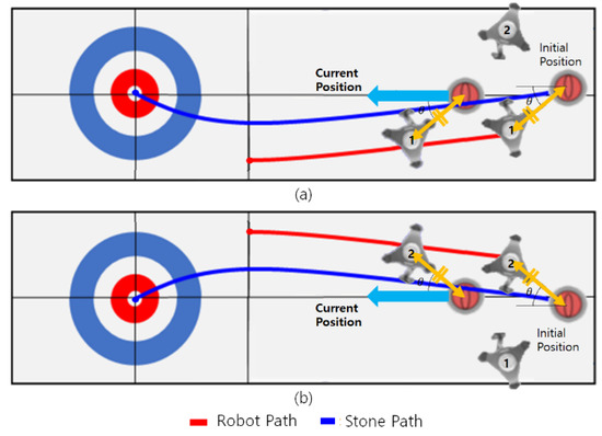
Figure 1.
(a) Movement of the left sweeper robot. (b) Movement of the right sweeper robot.
Firstly, a target path of the curling stone is received according to the strategy through TCP/IP communication from the main server. Based on this path, the initial path is generated by considering the formation of the curling stone and the two sweeper robots using Equation (7).
The angle between the curling stone and the robot on the x-axis is set by considering the speed of the curling stone. Using the θ, the initial paths of the two sweeper robots are finally generated.
To maintain the formation of the stone and the robot, the robot has to maintain the angle between the stone and the robot. If the formation changes due to the change of ice state or other external conditions, the robot must move to the initial formation to maintain the formation.
The distance and angle between the robot and the curling stone are determined using data from the lidar sensor to copy with the change due to external conditions as described in Equation (7). Since we know the location of the curling stone, we can use the information from the lidar sensor to locate the current robot at the desired position. The position of the robot can be obtained by Equation (7).
3.2. Actual Stone Position Estimation
Two methods are applied to estimate the actual curling stone position accurately. First, the position of the distance and direction to the curling stone is estimated by using the lidar sensor attached to the lower part of the sweeper robot [7]. The curling stone estimation method using the lidar sensor may cause an error by recognizing an object with a curvature similar to the stone as a curling stone [8,9]. To make up the above error, the position of the curling stone is estimated by using the camera image and Kalman filter. The data are used after verifying the validity of the location estimated by the lidar by comparing the location estimated by the lidar with the location estimated by the camera image and Kalman filter.
The method using the lidar sensor has the advantage of estimating the location of the curling stone with high spatial resolution with a small amount of calculation. In this paper, the coordinates of the data obtained by the lidar sensor are clustered to distinguish the curling from other objects. In this cluster, a circumcircle is obtained by using the starting point, the middle point, and the end point. By comparing the radius of a circumcircle with the radius of the actual curling stone, we can determine whether it is a curling stone or not. The algorithm for estimating the curling stone position using the lidar sensor is shown in Figure 2a.
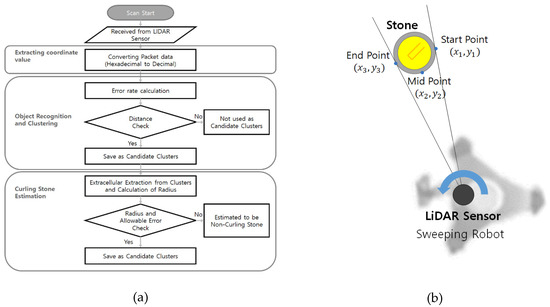
Figure 2.
(a) Clustering algorithm using light detection and ranging (lidar). (b) Three points of cluster.
We obtain a circumcircle of the triangle from the start, middle, and end points of the cluster derived from the clustering process as shown in Figure 2b. The formula for obtaining a circumcenter is described in Equation (8).
The radius of the circle is estimated by calculating the coordinate values of a circumcenter, that is, the center estimated coordinate values of the curling stone and the distance from the starting point in the cluster. The value obtained using Equation (8) is called by the theoretical value of the radius of the circle, and the formula for calculating the theoretical value is shown in Equation (9):
The second method is to estimate the actual curling stone location using the camera image and Kalman filter. An error between the image coordinates and the actual coordinates is generated by the computation time and the communication delay to estimate the curling stone position using the image coordinates.
The x, y coordinates of the curling stone obtained from the image coordinates and the running speed of the current robot are applied to the Kalman filter to estimate the coordinates of the current curling stone using Equation (10):
This error is corrected using a Kalman filter on the coordinate values. The coordinates of the current curling stone are estimated by applying the x, y coordinates of the curling stone obtained from the image coordinates and the running speed of the current robot to the Kalman filter. The Kalman coefficient according to the system model is obtained using the block diagram as shown in Figure 3 [10,11,12].
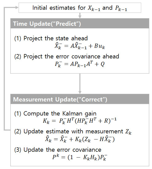
Figure 3.
Kalman filter block diagram.
3.3. Real-Time Path Planning
The path of the curling stone is estimated by weighting the TAES and the target path based on the estimated stone location and the previous path. It is possible to predict the position of the next curling stone by summing the weights of the slopes moving in the direction to reduce the error by comparing the slope between the current coordinates and the strategic coordinates. Since the path of the curling stone is in the form of a curve rather than a straight line, the algorithm is applied with a weight in consideration of this characteristic. This path prevents slippage due to the sudden change of direction of the robot and to following the movement of the curling stone. After estimating the slope to the next route, we can calculate the next expected coordinate with that slope that is obtained using Equation (11):
When the variable ratios of m1 and m2 are large in Equation (12), a suitable path may be generated by changing the weights of m1 and m2. The relationship between x3 and y3 corresponding to the expected coordinates is shown in Equation (12):
Since there are two unknown variables, we need one expression to find the exact value and estimate the other point through x or y coordinates. In addition, the relation between x3 and y3 can be found from the current stone velocity as shown in Equation (13):
3.4. Revised Movement Path of the Robot
The change of the curling stone’s path due to ice quality results in path error of the robot when compared with the expected path. Since the path error generated at this time inherently accumulates, the robot does not reach the final destination. To reduce the error, the sweeping process of the sweeper robot is processed by using a path generation algorithm for returning as shown in Figure 4. If the actual curling stone path crosses the path error threshold compared with the expected path, a path return is required. The blue line and the red line are the expected stone path and the actual stone path, respectively. When the threshold is exceeded, the sweeper robot sweeps the curling sheet to restore the curling stone. As a result, the changed path regenerates the return path as the green line in Figure 4 to regenerate the path for the stone to return to the expected path.
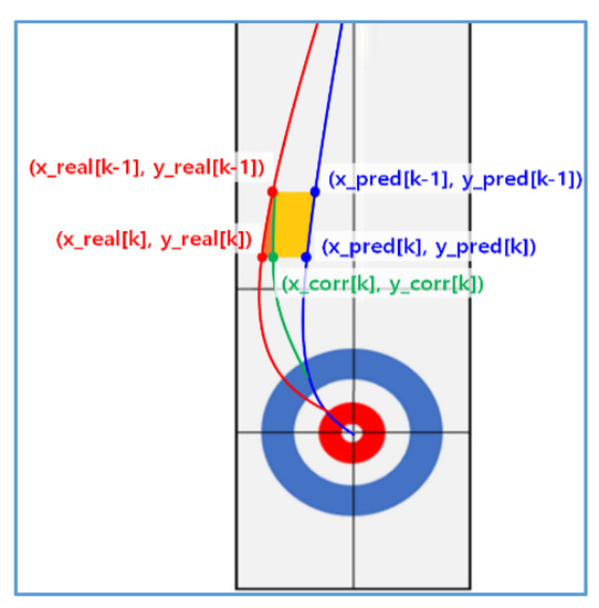
Figure 4.
Regenerated route to return to expected route.
Path generation for return uses a proportional area as shown in Figure 5a to predict a new path with coordinates that change during sweeping. The formula for calculating the area to be moved in order to return is given by Equation (14):
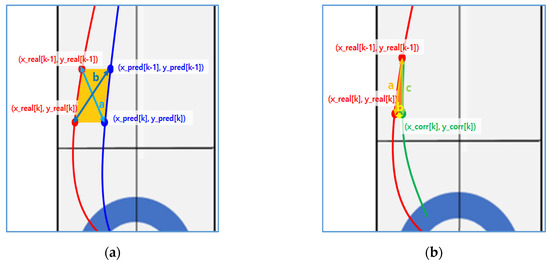
Figure 5.
(a) Return path generation using proportional area. (b) Area changed after path travel.
Therefore, the total area to be moved is given by Equation (15):
Figure 5b shows the area changed after the movement. The formula for calculating the area changed after the movement is described in Equation (16):
As a result, the total width moved is given by Equation (17):
When the sweeping is performed by using the above formula, the return path can be generated by predicting the change of movement.
4. Experiment
Due to the change in the friction coefficient of the curling arena sheet which varies in real time, the curling stone is difficult to predict the movement in the expected path of the initial stone. It is necessary to predict the change of the curling stone to generate the path of the sweeper robot and return the stone by sweeping the target path. Since it is impossible to use the general equation of motion due to the change of the friction coefficient of the curling sheet, we conducted the following experiment to predict the change of the curling stone as similarly as possible.
4.1. Stone Extraction Experiment with Rider Sensor Using Clustering Algorithm
Figure 6 is a photo of experiments in a real curling arena environment. For the sweeper robot to sweep according to the change of the curling stone movement, the actual curling stone position is checked and compared with the expected path. The data on location of the curling stone measured by a lidar sensor were clustered using the algorithm introduced in Figure 2a. Figure 7a which depicts the distance from lidar to the curling stone, shows that the circumference of the curling stone measured according to the actual distance changes. The experimental result for moving stone shows that the above algorithm works well regardless of the distance between lidar and curling stone. When the curling stone is triggered from the throwing robot, the stone moves to the end point in the form of a curve. In this process, the sweeper robot tracks the curling stone according to the location of the curling stone and determines whether or not to sweep. Figure 7b shows the results of the experiment that tracks a moving curling stone based on curling stone recognition. Experiments confirmed that the normal experiment proceeded as a result of recognizing the curling stone by tracking the moving curling stone using the algorithm of Figure 2a.
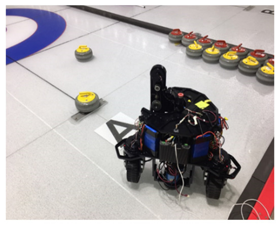
Figure 6.
Experiment on curling stone measurements in an actual curling field.
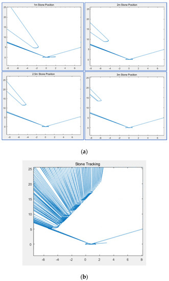
Figure 7.
(a) The distance between curling stone and lidar. (b) Curling stone tracking using an algorithm.
From the data on the position of the curling stone through the lidar sensor, it is possible to estimate the curling stone position in real time by reducing the computational time required to estimate and track the curling stone. Since the lidar sensor does not recognize color, it can recognize objects well except those shaped like curling stone.
4.2. Real-Time Curling Stone Data Extraction Experiment Using Kalman
This experiment was to predict actual data by using a Kalman filter. It was an experiment to obtain efficient shot data path in the obstacle-free space. Therefore, the data were not related to the shot used in the actual game.
Figure 8 depicts a graph of data extracted using Kalman filter based on actual data. The real trajectory graph means the data received from the image, and the Kalman prediction graph is the actual curling stone coordinates extracted using the Kalman filter.
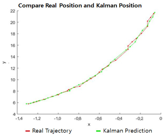
Figure 8.
Real trajectory and Kalman prediction.
4.3. Experiment with Trend-Adjusted Exponential Smoothing
The path of the curling stone is predicted from its position data obtained from the above experiments. Figure 9 extracts 100 data for the stone to move to the next step using 100 real position data when α = 0.3 and β = 0.1 with TAES. When more than 100 data were predicted by experiments in various cases, the error rate with the actual data was large, and the subsequent path estimation was calculated by using target path conversion using Equation (6). Table 1 shows a part of the result of predicting 100 actual data using 100 data. From the left, it shows actual data (x, y), trend adjusted exponential data (x, y), and error rate (actual data – trend-adjusted exponential). Figure 9 and Table 1 explain that a small error rate is generated when 100 data are extracted using TAES from 100 actual data.
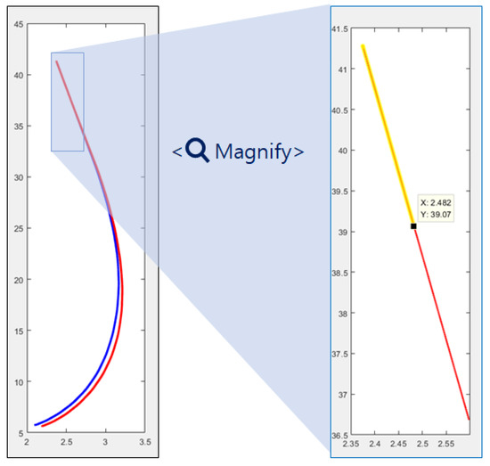
Figure 9.
Trend-adjusted exponential smoothing (TAES) graph.

Table 1.
TAES data.
4.4. Experiment on the Creation of Curling Stone Return Path Using Return Path Algorithm
When comparing the predicted route with the actual driving route through TAES, there are three major sweeping cases due to the error of the two routes, as shown in Figure 10a–c. First, sweeping is performed by comparing the speed of the curling stone when the current curling stone is equal to the expected coordinate interval. Second, when the current curling stone is pointing to the right of the target coordinate, sweeping in the left area is needed to return the curling stone moving to the right to the prediction path. Third, the current curling stone is to the left of its original expected coordinates. In this case, sweeping of the right area is needed to return the curling stone moving to the left to the prediction path. Sweeping is performed when the threshold value is exceeded using the following number of cases, and the path of the sweeping robot is regenerated based on the changed path of the curling stone.
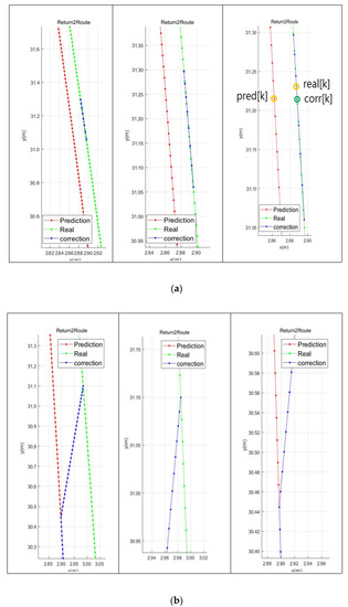
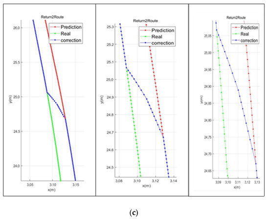
Figure 10.
Experimental results in case of (a) actual coordinates slower than expected. (b) Actual coordinates to the right of expected coordinates. (c) Actual coordinates to the left of expected coordinates.
Figure 11 shows a game of actual curling sheet using the above algorithm. The path of the sweeping robot was generated as the basis of the initial expected path, and the location of the curling stone was identified in real time, and the sweeping was performed by comparing with the expected path. In the real game, an error within 2 cm between the arrival point of the curling stone and the expected arrival point of the stone was generated.
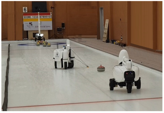
Figure 11.
Experiment on creating a return path using the return path algorithm in an actual curling field.
5. Conclusions
Using the data on the path prediction algorithm of the curling stone proposed in this paper, the sweeper robot plans its path for sweeping. By modifying the path closer to the target of the curling stone through the target, the robot’s path is also modified accordingly. In fact, there are many technical problems to solve in the robot curling game. One of the most important problems results from unpredictable movement of curling stone because the curling sheet is so sensitive to environmental factors such that even small changes have a significant impact on the movement of curling stone. Thus, in order to solve this problem, we used trend adjusted exponential smoothing, a time series analysis using trends, was used to predict curling stone paths in real time.
As a result of experimenting through the throw of the curling stone in the actual curling sheet, the sweeping robot moved according to the initial target path. It was confirmed that the stone’s path was predicted in real time through the experiment. In addition, when the estimated path is different from the target path because the speed is slow or the moving direction is different from the target path, the path is corrected by sweeping the curling sheet. Using the re-predicted path of curling stone, the robot’s path is re-planned.
In the experiment, the sweeper robot was designed to stop the sweeping before the opposite hog-line in the direction of travel. Since the sweeping robot used in the experiment was relatively large in size, it was sometimes difficult to sweep the sheet depending on the location of the curling stones. Future research includes designing compact sweeping robot with a different structure to solve the problem mentioned above.
Author Contributions
Conceptualization, H.B.; Investigation, J.G., H.K. and H.B.; Project administration, J.G. and S.L.; Software, J.G. and H.K.; Supervision, S.L.; Writing—original draft, J.G. and H.K.; Writing—review & editing, J.G. All authors have read and agreed to the published version of the manuscript.
Funding
This work was supported by the Basic Science Research Program, through the National Research Foundation of Korea, Ministry of Science, under Grant 2017R1D1A3B04031864.
Conflicts of Interest
The authors declare no conflict of interest.
References
- Charles, C.H. Forecasting seasonals and trends by exponentially weighted moving averages. Int. J. Forecast. 2004, 20, 5–10. [Google Scholar]
- Everette, S.G., Jr.; McKenzie, E.D. Forecasting trends in time series. Manag. Sci. 1985, 31, 1237–1246. [Google Scholar]
- Zhang, J.; Singh, S. Low-drift and real-time lidar odometry and mapping. Auton. Robot. 2017, 41, 401–416. [Google Scholar] [CrossRef]
- Wa̧sik, A.; Ventura, R.; Pereira, J.N.; Lima, P.U.; Martinoli, A. Lidar-based relative position estimation and tracking for multi-robot systems. In Proceedings of the Robot 2015: Second Iberian Robotics Conference, Lisbon, Portugal, 19–21 November 2015. [Google Scholar]
- Lohani, A.K.; Kumar, R.; Singh, R.D. Hydrological time series modeling: A comparison between adaptive neuro-fuzzy, neural network and autoregressive techniques. J. Hydrol. 2012, 442, 23–35. [Google Scholar] [CrossRef]
- Williams, T.M. Adaptive Holt—Winters Forecasting. J. Oper. Res. Soc. 1987, 38, 553–560. [Google Scholar]
- Shackleton, J.; Van Voorst, B.; Hesch, J. Tracking people with a 360-degree lidar. In Proceedings of the 2010 7th IEEE International Conference on Advanced Video and Signal Based Surveillance, Boston, MA, USA, 29 August–1 September 2010. [Google Scholar]
- Wang, Y.; Chao, W.L.; Garg, D.; Hariharan, B.; Campbell, M.; Weinberger, K.Q. Pseudo-lidar from visual depth estimation: Bridging the gap in 3d object detection for autonomous driving. In Proceedings of the IEEE Conference on Computer Vision and Pattern Recognition, Long Beach, CA, USA, 16–20 June 2019. [Google Scholar]
- Lee, J.H.; Bae, H.S.; Gwon, J.H.; Kim, N.H.; Albina, K.; Lee, S.G. Estimation of Curling Sheet Friction Factor by Pixelization. In Proceedings of the 2018 37th Chinese Control Conference (CCC), Wuhan, China, 25–27 July 2018. [Google Scholar]
- Chen, B.; Liu, X.; Zhao, H.; Principe, J.C. Maximum correntropy Kalman filter. Automatica 2017, 76, 70–77. [Google Scholar] [CrossRef]
- Moore, T.; Daniel, S. A Generalized Extended Kalman Filter Implementation for the Robot Operating System; Intelligent Autonomous Systems 13; Springer: Cham, Switzerland, 2016; pp. 335–348. [Google Scholar]
- Houtekamer, P.L.; Zhang, F. Review of the ensemble Kalman filter for atmospheric data assimilation. Mon. Weather. Rev. 2016, 144, 4489–4532. [Google Scholar] [CrossRef]
© 2020 by the authors. Licensee MDPI, Basel, Switzerland. This article is an open access article distributed under the terms and conditions of the Creative Commons Attribution (CC BY) license (http://creativecommons.org/licenses/by/4.0/).