FPGA-Based Doppler Frequency Estimator for Real-Time Velocimetry

Abstract

In range-Doppler ultrasound applications, the velocity of a target can be measured by transmitting a mechanical wave, and by evaluating the Doppler shift present on the received echo. Unfortunately, detecting the Doppler shift from the received Doppler spectrum is not a trivial task, and several complex estimators, with different features and performance, have been proposed in the literature for achieving this goal. In several real-time applications, hundreds of thousands of velocity estimates must be produced per second, and not all of the proposed estimators are capable of performing at these high rates. In these challenging conditions, the most widely used approaches are the full centroid frequency estimate or the simple localization of the position of the spectrum peak. The first is more accurate, but the latter features a very quick and straightforward implementation. In this work, we propose an alternative Doppler frequency estimator that merges the advantages of the aforementioned approaches. It exploits the spectrum peak to get an approximate position of the Doppler frequency. Then, centered in this position, a centroid search is applied on a reduced frequency interval to refine the estimate. Doppler simulations are used to compare the accuracy and precision performance of the proposed algorithm with respect to current state of the art approaches. Finally, a Field Programmable Gate Array (FPGA) implementation is proposed that is capable of producing more than 200 k low noise estimates per second, which is suitable for the most demanding real-time applications.

1. Introduction

Doppler ultrasound is employed in several applications, like the monitoring of industrial processes [1,2], biomedical investigations [3], and non-destructive tests [4]. In pulse-wave Doppler ultrasound, the signal received among subsequent echoes includes information about the displacement—and thus the velocity—of the particles that originated the echo. Ideally, a target investigated with a frequency $F_T$, and moving at constant velocity $v$, produces a single-tone shift whose frequency $f_v$ is given by the well-known Doppler equation:

$$f_v=2\frac{v}{c}{F}_{T}cos(\theta )$$

(1)

where $c$ is the sound velocity and $\theta$ is the angle between the target trajectory and the ultrasound propagation [3]. Unfortunately, due to several phenomena like velocity broadening (in a fluid the adjacent particles move with slight different velocities), geometrical broadening (the ultrasound waves sourced by the finite transducer aperture reach the target with slight different angles $\theta$ [5]), or the transit-time broadening (the particle crosses the ultrasound beam in a finite time [6]), the Doppler spectrum is composed by a relatively large bandwidth instead of a single frequency tone.

Several methods have been proposed in literature about how to get the best estimate of the Doppler frequency $f_v$ from the measured Doppler spectrum. Some advanced techniques are based on the detection of the maximum frequency present in the Doppler spectrum [7,8], while others employ mathematical models of the spectrum [9]. The assessment of the spectrum centroid, i.e., the center of mass, is one of the most commonly used approaches:

$$f_v=\frac{{{\displaystyle \int }}_{-0.5}^{0.5}x·\mathrm{PSD}\left(x\right)dx}{{{\displaystyle \int }}_{-0.5}^{0.5}\mathrm{PSD}\left(x\right)dx}$$

(2)

where PSD is the Power Spectral Density of the Doppler spectrum in the normalized frequency range − 0.5 to + 0.5.

In real-time applications, where the Doppler frequency should be evaluated hundreds of thousands of times per second, Equation (2) is sometimes approximated with the frequency that corresponds to the position of the spectrum peak. As shown in the following part of the paper, this approximation allows an easily hardware implementation, but features a lower precision with respect to Equation (2).

In this work, an improved frequency Doppler estimator is presented. The estimator is implemented in the field programmable gate array (FPGA) included in a real-time ultrasound board [10]. The proposed algorithm takes advantage of the characteristics of both the full centroid and the peak estimators: it features the low calculation effort typical of the peak estimator and the reduced variability typical of the centroid estimator. Unlike Equation (2), which is calculated over the full Doppler spectrum range, the proposed algorithm calculates the center of mass in a reduced frequency span. The estimate is carried out with less calculations, which represents a significant advantage for the hardware implementation. A parameter is introduced to set the extension of the frequency range where the centroid is calculated. Ultrasound simulations based on specialized software running in Matlab (The Mathworks, Natick, MA, USA) are employed to optimize this parameter with respect to the features of the Doppler spectrum. Other experiments are carried out to investigate the estimator accuracy and precision, and to show how it compares to state of the art.

The hardware implementation of the estimator is described and evaluated by experiments. A Newtonian fluid flowing in a pipe is investigated through the Doppler board [10], where peak, full centroid, and the proposed estimator are implemented. The throughput of the three estimators is measured and the quality of the implementation is evaluated by comparing the Doppler frequency estimates calculated in hardware to the corresponding estimates obtained in Matlab. Experiments show that the proposed estimator is capable of producing more than 200 k estimates per second with a mathematical noise below −150 dB, high accuracy, and precision.

2. Background and State-of-the-Art

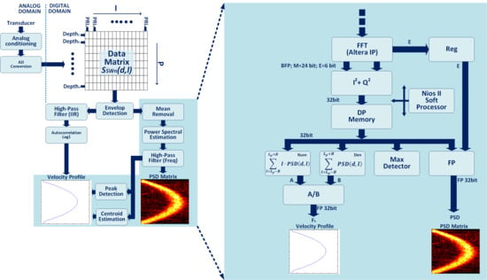
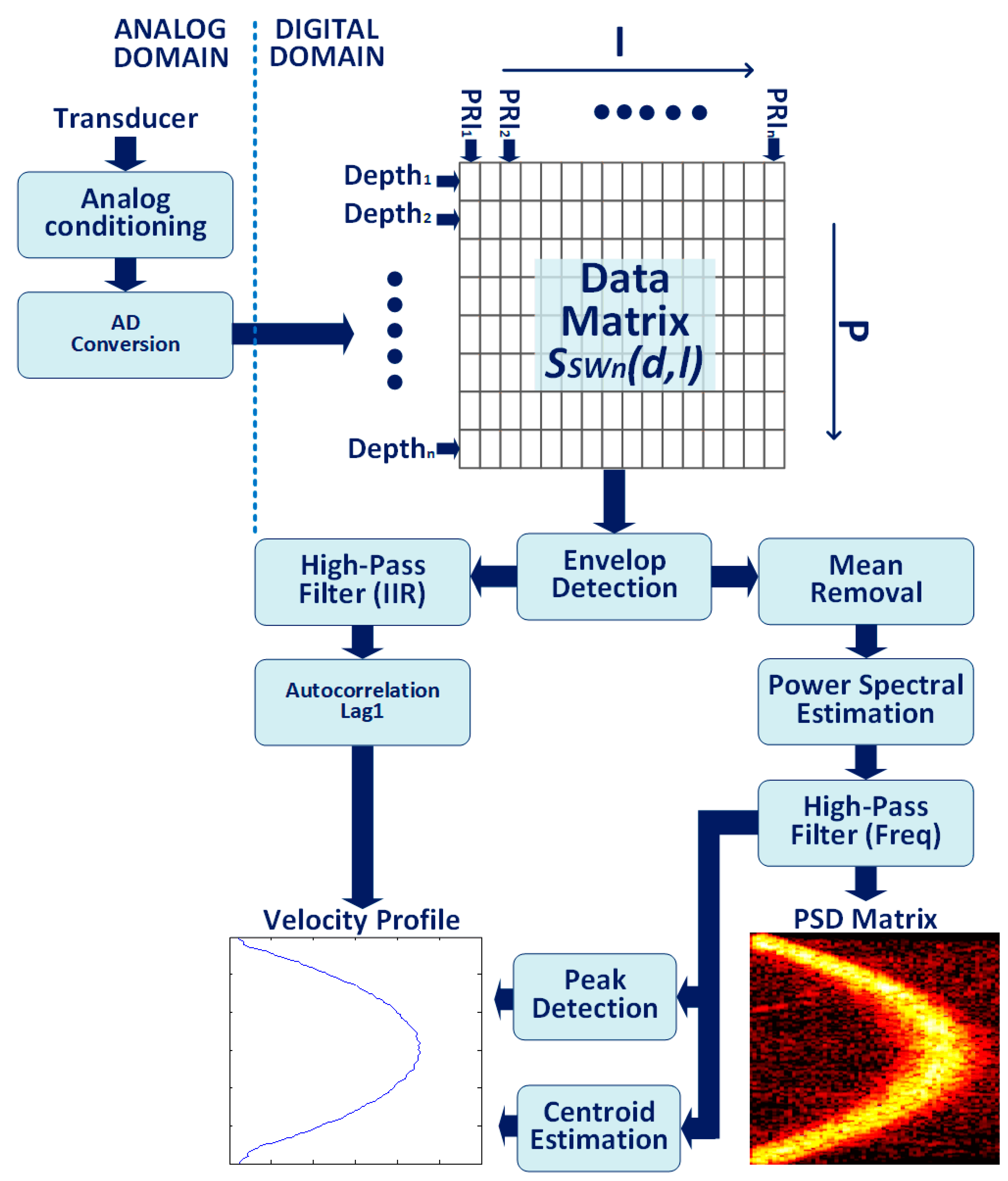
2.1. Doppler Processing Data Path Overview

General details of the data processing employed in Pulse-Wave ultrasound can be found in several papers and books, for example References [3,10,11,12]. Here a brief resume is reported to help readers with the subject, and to highlight the parts most relevant for the comprehension of the proposed algorithm.

In a pulse-wave Doppler system a burst of ultrasound waves of frequency $F_T$ is transmitted [13] in the fluid to be investigated by high-voltage pulsers [14] every pulse repetition interval (PRI). The ultrasonic burst travels in the medium at velocity c, and when it hits a scatterer, part of its energy is reflected towards the transducer. If the scatterer moves at velocity v, the echoes from subsequent transmissions are returned from slightly different positions. A phase-shift is thus observed in the received echoes. In particular, the phase rotation of echoes from subsequent PRIs corresponds to the frequency $f_v$ described quantitatively by the Doppler Equation (1).

The echoes received by the transducer are analog conditioned in the system front-end through filtering and amplification, and analog-to-digital (AD) converted at rate $F_c={\raisebox{1ex}{$1$}\!\left/ \!\raisebox{-1ex}{$T$}\right.}_c$ (see Figure 1 top-left). From now on, the calculations are typically performed through digital devices, like digital signal processors (DSP) or FPGAs.

The stream of sampled data is subdivided in PRIs sections of length $T_{Pri}=k_M·T_c$, where $k_M$ is the number of samples in each section. This process is formalized by considering the signal sampled at time $t=d·T_c+l·T_{Pri}$, and stored in the bidimensional matrix $s_{SWn}\left(d,l\right)$ (Figure 1 top-right). The row index, $d$, is typically named the ‘fast-time’ index and is in ranges of $0<\mathrm{d}<k_M$, while the column index, $l$, counts the PRIs and is typically named the ‘slow-time’ index. In this notation, the $d$-index represents the ‘depth’, i.e., the distance from the transducer [15]. Data sampled at same $d$ behave in the same way, and thus are similarly affected by the phase shift described above, which can be detected by an analysis along the $l$-index.

The signal segments stored along the columns of the matrix are processed for signal envelop detection (Figure 1 middle). Hilbert transform or coherent demodulation is employed [16]. The latter operation, used in this work, is performed by multiplying the signal for the complex sequence $e^{-2\pi i{f}_{T}d{T}_c}$ and by applying a low-pass filter with cut-off frequency $f_{LP}$. This filter affects the axial resolution and is typically tailored to the bandwidth of the transducer.

$$s_{SWDn}\left(d,l\right)=s_{SWn}\left(d,l\right)·e^{-2\pi i{f}_{T}d{T}_c}$$

(3)

The elaboration proceeds with the estimation of the Doppler frequency. This information is encapsulated in the sequence of samples stored in $s_{SWDn}\left(d,l\right)$, when considered at the same $d$ index, i.e., at the same distance from the transducer. Different strategies are possible, as sketched by the 2 alternate paths visible in Figure 1 bottom. The left path includes high-pass filtering [17] and autocorrelation (Figure 1 bottom-left). Alternatively (Figure 1 bottom-right), the PSD is calculated [18], followed by peak detection or full centroid estimation. Autocorrelation is specifically employed in applications where the PSD is not necessary. This paper is focused on methods based on PSD. Details of each step are provided in the following sections.

2.2. Power Spectral Estimation

The power spectral density distribution of the Doppler spectrum is obtained by processing the demodulated data $s_{SWDn}\left(d,l\right)$ by means of spectral estimators. Data are organized in ‘packets’ defined like:

$$\overline{P}\left(d,l,L\right)=\left[s_{SWDn}\left(d,l\right), \dots \dots ,s_{SWDn}\left(d,l+i\right), s_{SWDn}\left(d,l+L-1\right)\right]$$

(4)

where L is preferably a power of 2. A simple high-pass filter (at least the mean must be removed), is followed by windowing and Fast Fourier Transform (FFT) [19]. The use of more sophisticated adaptive estimators instead of FFT have been reported in literature as well [15,20,21]; however, more sophisticated adaptive estimators require a higher calculation power that makes the real-time hardware implementation more problematic.

This procedure is applied to all the depths of the demodulated data matrix $s_{SWDn}\left(d,l\right)$, for obtaining the corresponding sequences of power spectral density lines:

$$\mathrm{PSD}\left(d,k,F\right)=\Gamma \left\{\overline{P}\left(d,F·L·\left(1-w\right),L\right)\right\}$$

(5)

where $d$ and $k$ are the depth and frequency index, respectively, $\Gamma \left\{x\right\}$ is the power spectral estimator employed (e.g., FFT²(x)), $F$ is the frame index that accounts for the matrix sequence, $w$ is the overlap percentage of successive data packets ($0\le w<1$). For example, in case of $L$ = 128, $\Gamma \left\{x\right\}={\mathrm{FFT}}^2\left(\mathrm{x}\right),$ $w$ = 0.5, the first 128 demodulated data $s_{SWDn}\left(d,l\right)$ (0 < $l$ < 127) are processed through a 128-poinf FFT for every depth $d$. The squared output represents the first ($F$ = 0) output frame, i.e., the first spectral power density matrix. From now on, every new 64 PRIs, the last $L$ = 128 data (w = 0.5, i.e., 50% overlap) are processed for generating the next frames ($F$ = 1,2,3, etc.).

An approximated high-pass filter (clutter filter) can be applied easily in the frequency domain by removing the lower region of the PSD matrices. The performance of this filter is lower with respect to a full time-domain implementation (e.g., a Finite Impulse Response (FIR) filter). Nevertheless, the performance is sufficient for the application purpose [22] and it can be implemented efficiently in hardware. The final PSD matrix, which is color coded, represents an intuitive picture of the flow profile present in the pipe or the vessel (see, for example Figure 1 bottom-right). The rows report the Doppler shifts, which are proportional to the flow velocity, and the columns report the depths inside the pipe or vessel.

Once the PSD matrix is available, the Doppler frequency is obtained by estimating the centroid frequency or, simply, by taking the spectral peak.

2.3. Spectral Peak

The simplest Doppler frequency estimator is the peak estimator. In this case, the Doppler frequency is approximated by the position where the spectrum power features the maximum amplitude:

$$n_p:\mathrm{PSD}\left(\mathrm{d},n_p\right)=\mathrm{MAX}\left\{\mathrm{PSD}\left(d,l\right),0 \le l<\mathrm{L}\right\}.$$

(6)

The estimator requires L − 1 comparison only. It can be implemented in hardware with a single comparator used serially L − 1 times.

2.4. Centroid Frequency Estimation

The estimator basically calculates the ‘center of mass’ of the spectrum (2). In the discrete domain it can be implemented as:

$$n_d=\frac{{{\displaystyle \sum }}_{l=1}^{\mathrm{L}-1}l·\mathrm{PSD}\left(d,l\right)}{{{\displaystyle \sum }}_{l=1}^{\mathrm{L}-1}\mathrm{PSD}\left(d,l\right)}$$

(7)

where $\mathrm{PSD}\left(d,l\right)$ is the power spectrum density bin of index l (1 < l < L) calculated at depth d. Please note that the 0-frequency (l = 0) is excluded from the calculation. The accuracy of this estimator is high, but requires L − 1 multiplications, 2(L − 1) additions, and a division for each depth d, where L is the number of frequency samples of the PSD.

An approximated high-pass filter can be easily implemented by excluding, in addition to the 0-frequency bin, a wider low-frequency region. For example, Equation (7) can be modified as follows:

$$n_d=\frac{{{\displaystyle \sum }}_{l=L_m}^{L-L_m}l·\mathrm{PSD}\left(d,l\right)}{{{\displaystyle \sum }}_{l=L_m}^{\mathrm{L}-L_m}\mathrm{PSD}\left(d,l\right)}.$$

(8)

In this version the bins $-L_m<l<L_m$ are simply ignored. As anticipated above, the performance of this filter is limited, but remains sufficient for most applications.

3. The Proposed Method

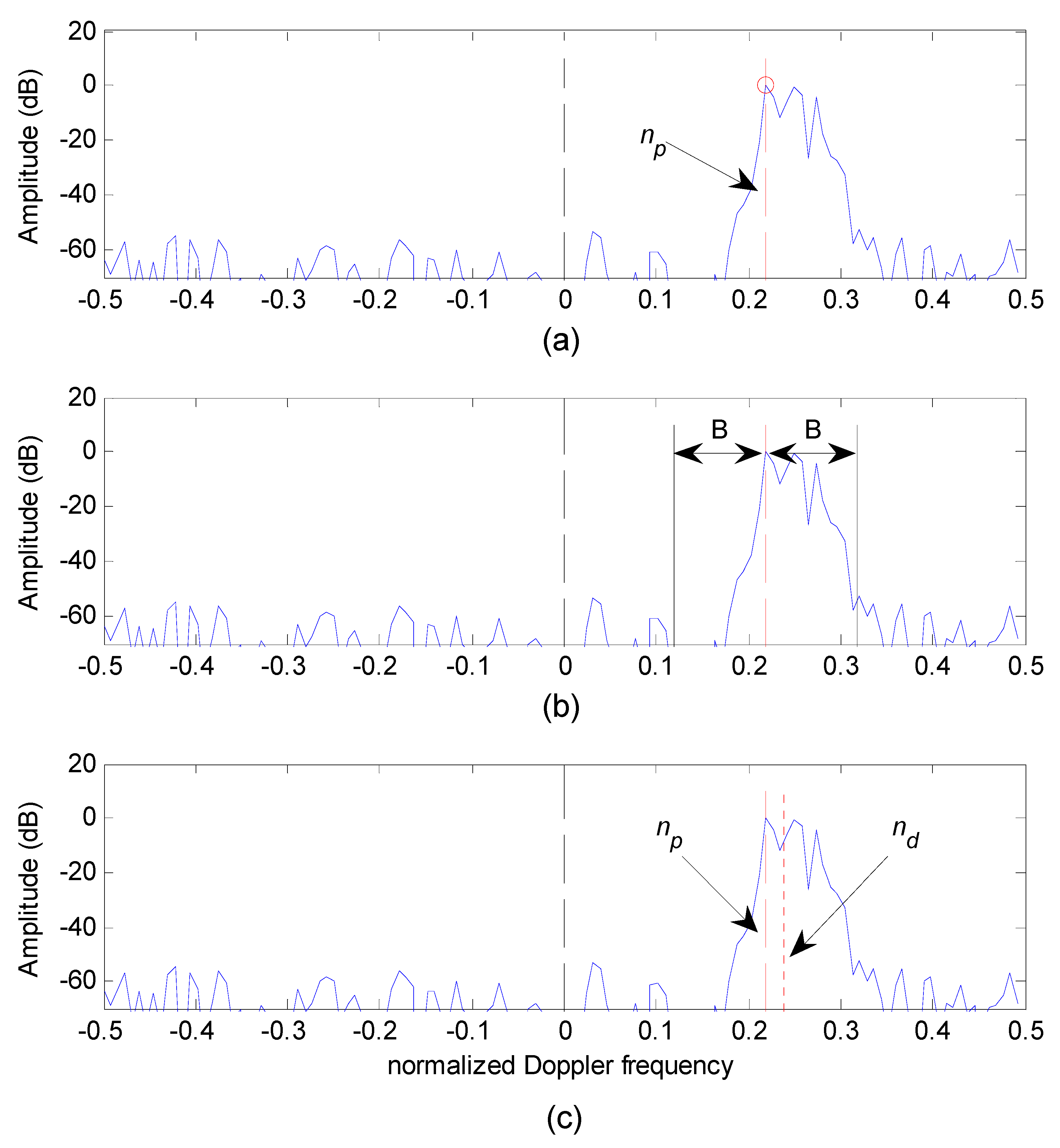
3.1. Method Basics

In this work we propose a modified Doppler frequency estimator optimized for the hardware implementation in real-time Doppler systems. The method is designed as part of the effort to merge the low calculation requirement of the peak estimator with the accuracy and precision of the centroid estimator. The proposed estimator processes the PSD of the Doppler spectrum estimated with a L-point FFT according to the following steps:

(a)

The peak estimator (6) is first applied to obtain $n_p$;

(b)

The frequency interval [$n_p-B,n_p+B$], centered on $n_p$ and of extension 2B + 1 is considered. More details on B are given below.

(c)

The centroid frequency $n_n$, output of the estimator, is estimated in the region located in previous step.

The process is clarified with an example. The 3 panels of Figure 2 report a typical Doppler PSD produced by a scatterer moving at 0.5 m/s investigated by transmitting 3.5 MHz ultrasound bursts. The PSD is obtained by a L = 128 point FFT, and it is represented in the normalized frequency range −0.5 to +0.5. The scatterer movement produces a rough bell-shaped spectrum approximatively located in the region 0.21, 0.35. In this example, the background noise is about 60 dB below the spectrum peak.

In the first step, the FFT bin corresponding to spectrum peak is located by applying the peak estimator (6). The peak is reported by the red circle in Figure 2a, and the corresponding frequency $n_p$ = 0.22 is highlighted by the vertical dashed segment. The detected frequency is considered a first approximation of the Doppler frequency.

In the second step a frequency interval of extension 2B + 1 bins is centered around the $n_p$ frequency. In the example B = 12 bins is chosen, which corresponds to a normalized frequency interval of B/L = 12/128 ≃ 0.1. More details about the selection of the B value are given in the next section. Figure 2b reports the 2B + 1 frequency interval centered in $n_p$. The interval includes approximatively the Doppler bandwidth detectable above the background noise.

In the last steps, the centroid estimator is applied in the frequency region defined in the previous step. The application of the estimator is different with respect to the full centroid calculation (7). In fact, in Equation (7), the whole frequency range is considered, while here the calculation is focalized on the reduced frequency interval centered in the position of the peak. In this case, the centroid estimation is analytically expressed as:

$$n_d=\frac{{{\displaystyle \sum }}_{l=n_p-B}^{n_p+B}l·\mathrm{PSD}\left(d,l\right)}{{{\displaystyle \sum }}_{l=n_p-B}^{n_p+B}\mathrm{PSD}\left(d,l\right)}.$$

(9)

Figure 2c compares the final Doppler frequency estimate $n_d$ calculated by Equation (9) to the first estimate obtained with the peak estimator $n_p$. The frequencies are reported by dashed and dotted red vertical segments, respectively. In this example, the proposed estimator produces $n_d$ = 0.24. This value corrects the first frequency estimate by shifting the result towards the high frequencies. This behavior agrees with the shape and position of the Doppler bandwidth, whose area is visibly biased towards the higher frequency with respect to the $n_p$ estimate.

The proposed estimator requires L − 1 comparisons for the detection of the peak in step a), followed by 2B multiplications, 4B summations, and a division for the centroid calculation (see Equation (9)).

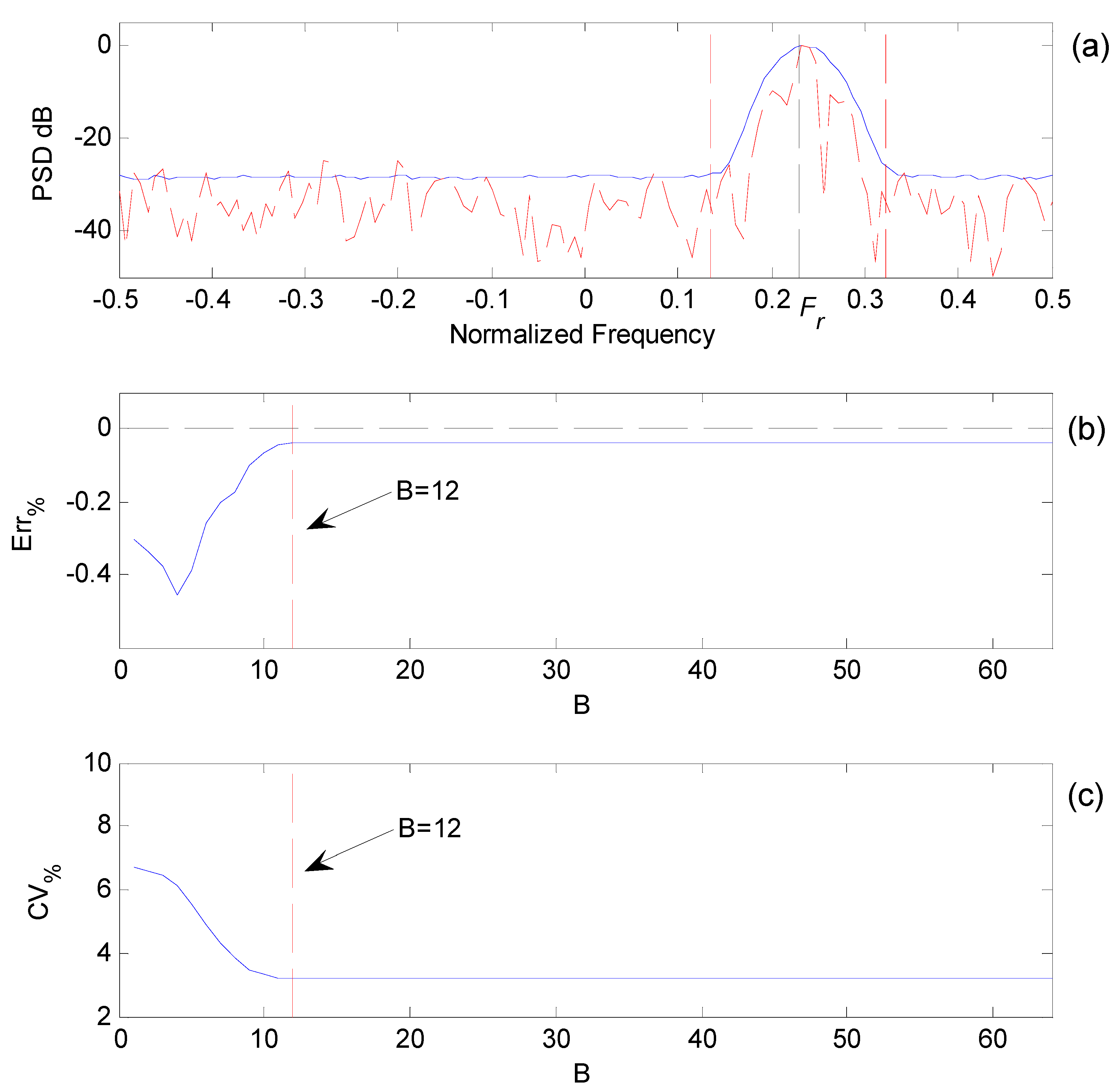
3.2. The B Parameter

In this section how the performance of the estimator depends on the parameter B is investigated. This study is based on ultrasound simulations carried out with Field II [23,24], a specialized simulator freely available at https://field-ii.dk. Field II, given the position of a set of scattering particles, the transducer characteristics, and the TX pulse, simulates the raw echo data received in each PRI. In this test, a piston transducer transmits in a 45 mm diameter pipe ultrasound bursts composed by 5 cycles at 3.5 MHz and PRI = 0.2 ms. The positions of the scattering particles are updated every PRI to mimic the typical parabolic profile of a Newtonian fluid flowing in a straight pipe. A peak velocity of 0.5 m/s is simulated. White noise generated in Matlab is added to the echo signal produced by the Field II simulator to achieve a Signal-to-Noise Ratios (SNRs) of 0 dB. The signal is further processed as described in Section 2.1 through a 128-point FFT (L = 128) to obtain the PSDs. 20,000 PRIs are generated, corresponding to more than 300 PSD matrices with 50% overlap (w = 0.5, 0 < F ≤ 300). According to the simulation parameters, the nominal normalized Doppler frequency is $F_r$ = 0.23.

The proposed estimator (9) is applied to the PSDs at the depth where the velocity reaches its peak of 0.5 m/s. The estimator is applied with the parameter B varying in its full range, i.e., 0 ≤ B < 63. The accuracy of the estimates is evaluated according to the following metrics:

$${\mathrm{Err}}_{\%}=\frac{mean\left\{F_s\left(\mathrm{F}\right),\mathrm{F}\right\}-F_r}{F_r}·100$$

(10)

where $F_s\left(F\right)$ is the Doppler frequency detected by the estimator under the test in the PSD of frame F, $F_r$ is the ground truth value obtained by the simulations, $mean\left\{F_s\left(\mathrm{F}\right),\mathrm{F}\right\}$ is the average of $F_s\left(\mathrm{F}\right)$ calculated over the available frames. The precision was evaluated through the Coefficient of Variability (CV_%):

$${\mathrm{CV}}_{\%}=\frac{std\left\{F_s\left(\mathrm{F}\right),\mathrm{F}\right\}-F_r}{F_r}·100$$

(11)

where $std\left\{F_s\left(\mathrm{F}\right),\mathrm{F}\right\}$ is the standard deviation of $F_s\left(\mathrm{F}\right)$ calculated in the available frames.

Figure 3 shows the results of the study. The top panel (a) reports the mean spectrum (blue curve), obtained by averaging the 300 available frames. An example of a single spectrum (red dashed curve) is superimposed. The vertical black segment reports the nominal Doppler frequency $F_r$ = 0.23. Figure 3b,c report, respectively, the mean error and the coefficient of variability calculated by Equation (10) and Equation (11). Both graphs present a similar trend: the worst performance is observed for low values of B. Performance improves with higher values of B until B reaches 12 (vertical red dashed segments). From now on, performance is stable at its maximum value. The frequency interval corresponding to B = 12 is highlighted in Figure 3a by the vertical dashed segments. The interval includes the Doppler frequencies detectable above the background noise.

This study suggests that the proposed algorithm produces the best performance when B corresponds to a frequency region that includes all of the Doppler frequencies present in the measured spectrum. Higher B values do not produce improvements. Since the calculation effort scales with B, the optimal choice of B is the lowest value that grants the best accuracy and precision. In this example, it corresponds to B = 12. Although this study is based on a specific example, the simulated Doppler spectrum is representative of a wide range of practical conditions. In conclusion, a value of B in the range 10–20 covers most of the practical cases.

3.3. Comparison of Proposed Method to Standard Methods

In this section, the proposed method is compared to the standard approaches employed in real-time applications, i.e., the peak and the full centroid estimator.

For this study, the ultrasound signals generated by Field II for the previous study have been used. White noise was added to achieve 6 different Signal-to-Noise Ratios (SNRs) levels, between −20 dB and +20 dB (see leftmost column in

Table 1. Accuracy and precision.

SNR	Peak Estimator		Full Centroid Estimator		Proposed
	$\mathbf{E}\mathbf{r}{\mathbf{r}}_{\mathbf{\%}}$	$\mathbf{C}{\mathbf{V}}_{\mathbf{\%}}$	$\mathbf{E}\mathbf{r}{\mathbf{r}}_{\mathbf{\%}}$	$\mathbf{C}{\mathbf{V}}_{\mathbf{\%}}$	$\mathbf{E}\mathbf{r}{\mathbf{r}}_{\mathbf{\%}}$	$\mathbf{C}{\mathbf{V}}_{\mathbf{\%}}$
−20 dB	−8.74%	51.1%	−68.3%	63.3%	−8.8%	50.7%
−15 dB	−0.38%	7.3%	−29.67%	31.9%	−0.11%	4.4%
−10 dB	−0.21%	6.9%	−2.38%	6.7%	−0.15%	3.2%
0 dB	−0.13%	6.8%	−0.04%	3.2%	−0.06%	3.2%
10 dB	−0.17%	6.8%	−0.04%	3.2%	−0.04%	3.2%
20 dB	−0.13%	6.7%	−0.04%	3.2%	−0.04%	3.2%

). The signals were processed as described in the previous sections to obtain the PSDs. These were further processed with the peak estimator (6), full centroid estimator (7), and the proposed estimator (9) with B = 12. The achieved accuracy and precision were evaluated with the metric (10) and (11), respectively. Results are listed in Table 1.

When the SNR is below −20 dB, all the tested algorithms fail (first row of Table 1). With SNR = −15 dB (second row), the centroid estimator is still not capable of producing reliable estimates, but peak and proposed estimators start to issue reasonable results. As long as the SNR increases (3rd and following rows of Table 1), the performance improves. In particular, peak estimator produces good results starting from −10 dB (${\mathrm{Err}}_{\%}$ ≃ 0.1%–0.2% and ${\mathrm{CV}}_{\%}$ ≃ 6.7%–6.9%); full centroid estimator features ${\mathrm{Err}}_{\%}$ = 0.04% and ${\mathrm{CV}}_{\%}$ ≃ 3.2% from 0 dB. The proposed estimator presents the best performance. In fact, it features a low error and high precision starting from –15 dB, and its precision is always better compared to the peak estimator.

These results are explained by the features of the typical ultrasound signal. The ultrasound signal is affected by the speckle noise [25], which produces temporal variation, which is visible in the example of Figure 2. This noise varies quickly in time, and successive spectra are affected by a completely different noise shape. The peak estimator is particularly prone to this noise, as confirmed by its relatively high variability (${\mathrm{CV}}_{\%}$ > 6.7% in Table 1), which is also present with a high SNR. On the other hand, the full centroid and the proposed estimators, which employ a weighted mean over a frequency region, are less sensitive to random variation of the spectra (${\mathrm{CV}}_{\%}$ ≃ 3.2% in Table 1).

Peak frequency estimator is affected by another limitation: its output values are limited to the exact positions of the FFT bins, i.e., they are quantized to L values over the whole spectrum range. In other words, the frequency resolution is 1/(PRI∙L) only. This limitation does not apply to full centroid or the proposed estimators.

Table 2. Calculation power for the estimators.

Operations	Weight	Peak Estimator L = 128		Full Centroid Estimator L = 128		Proposed Estimator L = 128 B = 12
Comparisons	1	L−1	127	-	-	L−1	127
Additions	1	-	-	2(L−1)	254	4B	48
Multiplications	2	-	-	L−1	127	2B	24
Divisions	16	-	-	1	1	1	1
Total Effort			127		524		239

reports the number of comparisons, additions, multiplications, and divisions required by each estimator, while the operations required by the other processing steps visible in Figure 1 (e.g., the FFT), are excluded here. The operations are reported as a function of L and B and for the typical values of L = 128 and B = 12 (left and right of the corresponding column). The weight (second column in Table 2) represents a heuristic value that accounts for the complexity of the operations in a generic hardware implementation. Comparisons and additions are considered for weight 1 because in FPGA, its hardware is quite simple. Multiplications require a more complex hardware, so their weight is set to 2. Divisions are the most complex, thus the weight is set to 16. A total effort is then estimated by summing each contribution calculated by the product between the number of operations and the corresponding weight. The result is reported in the last row of Table 2. The method that requires less hardware effort is the peak estimator, but this efficiency is achieved at the expanse of precision (see Table 1). Proposed algorithm features an optimal tradeoff: it presents better accuracy and precision than the full centroid estimator, and requires half of its hardware effort (239/524 = 45%).

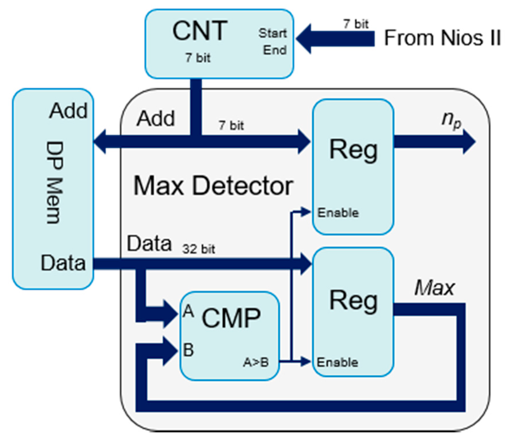
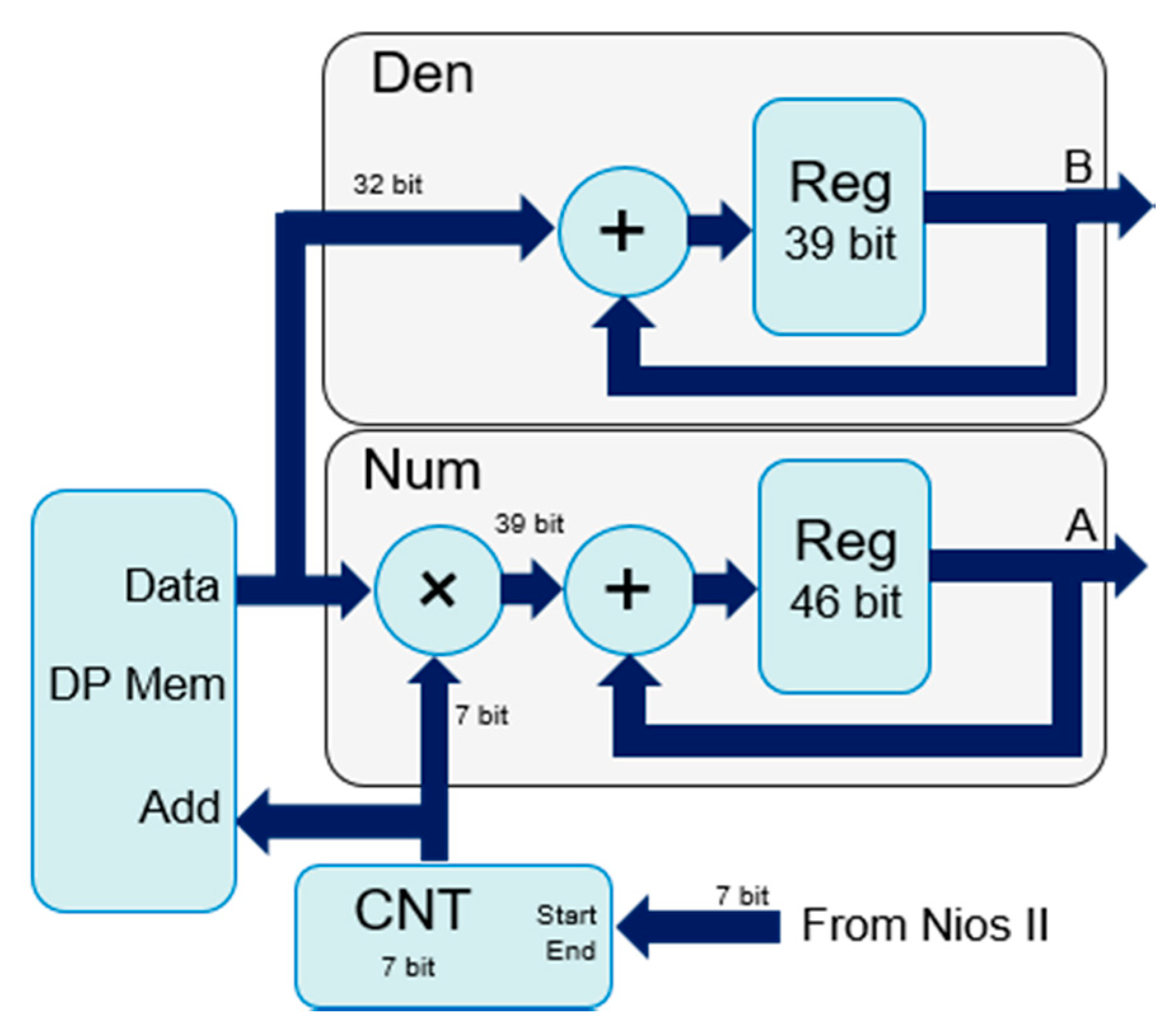
4. Circuit Architecture

The circuit was implemented in a FPGA of the Cyclone III family (Altera-Intel, San Jose, CA, USA). The FPGA is part of a complete ultrasound system designed for the investigation of fluids in industrial applications. More detail of the system and of the implementation of the full processing chain can be found in Reference [10], while this description is limited to the sections of interest for the frequency estimators. The circuit is sketched in Figure 4. A Nios II soft processor (IP from Altera-Intel), manages the sequence of operations and programs the processing modules by setting their registers. The section delimited by the dashed rectangle at the top left of the figure produces the PSDs. The modules delimited by the dashed rectangle located on the Figure bottom implement the frequency estimator. A dual port (DP) memory is used to transfer the PSD between the sections.

Data coming from the demodulator are processed through a 128-point FFT working on complex data (I,Q). The FFT is implemented by using the Altera-Intel Intellectual Property (IP) [26], configured with 24 + 24 bit input with “burst with quadruple output” architecture. Once its input buffer is loaded, the IP starts the FFT processing and produces the complex results in the output buffer. The 128-sample result is produced at 24 + 24 bit of mantissa and 6 bit for the exponent. The exponent applies to all the data block (block floating point representation), and is saved in a register for later use. Data are read from the FFT module and moved in the I² + Q² block (see Figure 4), where real and imaginary parts are squared and summed at 48 bit for obtaining the PSD. The 128 PSD samples are reduced to 32 bit and saved in the DP memory. When the 128 data block is completely moved in the memory, the FFT output buffer is empty, and the FFT starts loading and processing a new data block. A floating point converter (FP) is employed to output the PSD in floating point format.

The elaboration proceeds in the second section of the circuit with the estimation of the Doppler frequency from the PSD line present in the DP memory. The electronics implemented in this section is suitable for processing PSD data according to the 3 methods: the peak estimator (6), full centroid estimator (7), and proposed estimator (9). The modules for the Doppler frequency calculation include: the Max Detector, employed to locate the position of the PSD peak; the Num and Den, used to calculate the numerator and denominator of Equation (7) or (9); and a divisor (A/B) for the calculation of the quotient present in Equation (7) or (9). The Nios II processor switches among the 3 different estimators and tunes the parameter B of the proposed estimator by setting the processing module registers: the FPGA does not need to be reconfigured.

In order to process PSD data according to the proposed estimator, the Nios II first activates the Max Detector block, detailed in Figure 5. The Nios II sets the address generator counter (CNT) to scan the full address range (i.e., 0–127) of the DP memory, and zeros the Max register. PSD samples are sequentially read from the DP memory, and the comparator (CMP) triggers the enable signal when a value higher than that already stored in the Max register is found. The trigger activates the 2 registers that store the new value and its address, respectively. After 128 cycles, the whole DP memory is scanned, and the Max Detector block outputs $n_p$, i.e., the address (position in the spectrum) of the highest PSD sample. In the next step, the Nios II soft processor activates Num and Den modules to calculate numerator and denominator of (9). These modules are detailed in Figure 6. Nios II calculates $n_p$ − B and $n_p$ + B, and sets these values in the address generator (CNT) registers to scan the corresponding DP memory span. According to this architecture, the B value can be easily changed at the run time. The accumulation registers A and B are zeroes and the memory is read. As long as the PSD samples are read from the memory, they are accumulated in the B register (see the denominator of Equation (9)). Simultaneously, they are multiplied to the address and the result is accumulated in the A register (see the numerator of Equation (9)). The operation terminates after the programmed memory span is read, i.e., after $n_p$ + B − ($n_p-$ B) + 1 = 2B + 1 cycles. In the last step, the Nios II processor starts the A/B module. This module, composed by IPs of the Intel/Altera library, calculates the ratio and converts the result in 32 bit floating-point format. This ratio represents the final frequency estimate calculated according to Equation (9).

• When data is processed according to Peak estimator, the Nios II activates the Max Detector only to get $n_p$. When data is processed through full centroid estimator (7), the Nios II runs Num and Den modules on the whole PSD frequency range, followed by the A/B module.

5. Experiments and Results

The architecture presented in Figure 4 was implemented in the Cyclone III FPGA of the ultrasound board [10]. With the exception of FFT, the DP memory, and the A/B module, which are built with Altera-Intel IPs, all the other blocks are coded for the specific applications directly in VHDL. First, the modules were implemented separately for investigating the latency, maximum clock frequency, and the required FPGA resources. Then, they were connected according to the architecture of Figure 4 and they were employed to process data in real-time in Doppler acquisition. In this last configuration, the throughput and the mathematical noise were analyzed.

5.1. Modules Latency

The number of clock cycles needed by each module for processing a 128-sample data set is reported in

Table 3. Latency in clock cycles.

PSD Calculation (L = 128)
Block	Parameter	Latency (Clock Cycles)
FFT	TFFT	294
I2+Q2	TIQ	135
FP	TFP	135
Doppler Frequency Calculation
Block	Parameter	Peak Estimator L = 128	Full Centroid Estimator L = 128	Proposed est. L = 128; B = 12
Max Det.	TM	130	Not used	130
Num	TND	Not used	131	29
Den	TND	Not used	131	29
A/B	TD	Not used	16	16

. The FFT needs 294 cycles to load inputs, process data, and store results in its output buffer. I² + Q² and FP modules take 135 clock cycles for processing the 128-sample set, corresponding to 1 sample per clock in addition to 7 cycles needed for the initialization and the filling of their pipeline. Similarly, Max Detector processes 1 sample per clock in addition to 2 extra cycles, and Num and Den processes 1 sample per clock in addition to 5 extra cycles. The divisor performs the ratio and floating-point conversion in 16 cycles. First rows of Table 3 lists the number of clock cycles required by the FFT, I² + Q², and FP modules for the calculation of the PSD. The following rows of the Table compares the number of clock cycles required by the Max Detector, Num, Den, A/B modules when implementing the proposed (9), peak (6) and centroid (7) estimators, respectively.

5.2. FPGA Resources and Maximum Clock Frequency

The resources required by each module are listed in

Table 4. Resource utilization and frequency of each processing module in a Cyclone III FPGA.

Block	LEs	DSPs	Memory Bits	Max Clock Freq.
FFT	10,308	24	40,900	105 MHz
I2 + Q2	400	14	0	110 MHz
DP Mem	0	0	4096	210 MHz
Max Det.	70	0	0	150 MHz
Num	600	0	0	120 MHz
Den	600	0	0	120 MHz
A/B	230	0	0	110 MHz
FP	300	0	0	120 MHz

together with the maximum clock frequency the module can work at. FFT is the module with the lowest maximum frequency. This is expected, since FFT is the most complex block. Apart from the memory, which is a hardware IP, the highest frequency is achieved by the Max Detector.

5.3. Data Throughput

The modules were connected together like in Figure 4 and fed by a 100 MHz clock. For each module, a “Busy” signal was generated. Busy is high when the corresponding module is processing data, while it is low when the module is ready to accept a new data set. The processed data are available on the high-to-low transition for each module. A “DataValid” signal was added as well. It is asserted for a cycle when the final Doppler frequency estimate is ready. These signals were monitored by connectoing the board [10] to the Altera-Intel in-line debug tools through the Joint Test Action Group (JTAG) channel. The results of this analysis are reported in Figure 7 for the 3 frequency estimators. The horizontal axes report the clock cycles (see top scale in each panel); the origin is arbitrary set to the FFT start.

Figure 7a refers to the Peak estimator. The first 2 rows show the working cycles of FFT and I²+Q² modules while they calculated the PSD. The FFT restarted its calculation cycle when its output buffer was empty, a condition that occurred when the I² + Q² block had moved the data to DP memory. PSDs were calculated and stored in the DP memory at the maximum throughput T₁ allowed by the modules:

T₁ = T_FFT + T_IQ = 294 + 135 = 429 clock cycles.

(12)

Every time a PSD was ready, the Max Detector produced the results (Freq ready) after T_M = 130 cycles, as confirmed by the assertion of the DataValid signal (6th row). The Max detector was much faster than FFT and I² + Q² modules (429 against 130 cycles, see Table 3) and stalled for most of the time. The throughput was limited by the calculation of the PSD: a new frequency estimate was produced every T₁ cycles.

Figure 7b reports the signals for the full centroid estimator. In this case, the PSD calculation was slower with respect to Equation (12). In fact, the I² + Q² module did not start immediately at the FFT end not to overwrite data in the DP memory that are used by the FP module (see curved arrow). The throughput was here limited by the estimator operations. The clock cycles needed for producing every new frequency estimate were:

T₂ = T_M + T_ND + T_FP + T_IQ = 130 + 131 + 135 + 135 = 531.

(13)

The module A/B worked in parallel to FP, so it did not affect the timings to the point of achieving T_D < T_FP.

Figure 7c reports the signals for the proposed estimator. In this case, T_ND was much lower compared to the previous case, and the FP module completed its operations near the end of the FFT. Thus, the DP memory was free and I² + Q² started the calculations as soon as FFT ended, like in Figure 7a. In other words, the bottleneck was not the estimator, but the calculation of the PSD, as in the case of the Peak estimator, and Equation (12) applies again.

Table 5. Throughput of the frequency estimation for L = 128.

Estimator	T (Clock Cycles)	Throughput Estimates/s
Proposed B = 12	429	232 k
Full centroid	531	189 k
Peak estimator	429	232 k

summarizes the throughput of the architecture of Figure 4 for the 3 estimators considered here. When the Peak estimator is employed, the throughput is limited by the calculations of the PSDs, which depends on the performance of FFT; when the Full centroid estimator is used it represents the bottleneck. The proposed estimator is faster than the Full centroid, and the performance is limited by the PSD calculation, like for the Peak estimator.

5.4. Mathematical Noise

The ultrasound board was used to investigate a flow in a pipe of 40 mm diameter. In the pipe flowed a Newtonian suspension composed by 10 µm plastic spheres dispersed in demineralized and degassed water. The plastic particles were responsible for ultrasound scattering [27]. A focused piston transducer transmitted short bursts at 3.5 MHz every 500 µs. Received echoes were processed onboard in real-time through the 3 estimators considered in this paper. As detailed in Section 4, it was possible to switch among the different estimators by changing the operation sequence in the Nios II processor without reconfiguring the FPGA. The proposed estimator, in particular, was set with B = 12.

Raw data from the converters, calculated PSDs, and frequency profiles calculated by the proposed estimator where saved onboard and then downloaded to a PC for postprocessing and further analysis in Matlab.

An example of PSD matrix calculated by the board is reported in the left panel of Figure 8. The spectral power density, coded in colors in 40 dB dynamics, clearly shows the parabolic profile developed by the flow. The background noise is visible at about −30 dB. Reference PSDs were calculated in Matlab by using re-processing in its native 64-bit floating point representation the data acquired by the onboard AD converters. Onboard- and Matlab-calculated PSD were compared for the evaluation of the mathematical noise introduced by the FPGA calculations. The SNR, evaluated by computing the ratio between the power of the Matlab PSDs and the difference between Matlab and FPGA PSDs, was higher than 130 dB.

The middle panel of Figure 8 shows the frequency profiles calculated onboard with the proposed algorithm from the PSD matrix visible on the left. The frequency profiles calculated on board with the proposed estimator were compared to those calculated in Matlab starting from the same PSDs. The SNR, quantified in the same way as for the PSDs, resulted in a higher 150 dB. The right panel of Figure 8 shows, for example, the difference between the frequency profile reported in the middle panel and the corresponding profile calculated in Matlab.

6. Discussion and Conclusions

In this work, an efficient estimator for the detection of Doppler frequency from spectra has been presented. Its FPGA implementation was reported as well. The estimator exploits and merges the advantages of the peak and full centroid estimators, typically employed in real-time Doppler applications. The proposed estimator features an accuracy similar to or higher than that achieved by the full centroid estimator, and in addition allows a 50% (with B = 12) saving in calculation power (see Table 2).

The estimator employs the parameter B. Simulations allowed us to estimate B = 12 similarly to the optimal choice, at least in the presented case of study. Theoretically this value should be tailored to the extension of the “bell” of the spectrum. However, its exact value is not critical and a value between 10 and 20 is expected to fit most of the practical applications. Moreover, in the presented FPGA implementation, B can be changed at run-time, as well as among subsequent PSDs, if required. In a critical application, the Nios II can be programmed to calculate statistics like those that presented in Figure 3 to detect optimal B values.

Literature reports errors around 4%–10% for ultrasound measurements [28]. The error reported in this paper (Err_% < 1% in Table 1) is not in conflict with literature, since it was obtained in simulation, where most of the uncertainties present in real experiments are avoided [29]. On the other hand, simulation results confirm that the proposed estimator achieves a better accuracy with respect to peak estimator.

The presented FPGA architecture is suitable for the calculation of the 3 estimators without reconfiguration, with low resource utilization, and with a mathematical SNR higher than 150 dB. Moreover, with a 100 MHz clock frequency, more than 200 k PSD/s are calculated. This makes the estimator suitable for a wide range of demanding applications, like biomedical real-time blood flow investigations based on vector Doppler and plane waves [30], or analysis of industrial flow in large pipes where thousands of depths per frame are used [4].

References

1. Dong, X.; Tan, C.; Dong, F. Gas-liquid two-phase flow velocity measurement with continuous wave ultrasonic doppler and conductance sensor. IEEE Trans. Instrum. Meas. 2017, 66, 3064–3076. [Google Scholar] [CrossRef]
2. Kotzé, R.; Ricci, S.; Birkhofer, B.; Wiklund, J. Performance tests of a new non-invasive sensor unit and ultrasound electronics. Flow Meas. Instrum. 2015, 48, 104–111. [Google Scholar] [CrossRef]
3. Evans, D.H.; McDicken, W.N. Doppler Ultrasound Physics, Instrumentation and Signal Processing; Wiley: Chichester, UK, 2000. [Google Scholar]
4. Wiklund, J.; Stading, M. Application of in-line ultrasound Doppler-based UVP–PD rheometry method to concentrated model and industrial suspensions. Flow Meas. Instrum. 2008, 19, 171–179. [Google Scholar] [CrossRef]
5. Newhouse, V.L.; Varner, L.W.; Bendick, P.J. Geometrical spectrum broadening in ultrasonic Doppler systems. IEEE Trans. Biomed. Eng. 1977, 24, 478–480. [Google Scholar] [CrossRef] [PubMed]
6. Newhouse, V.L.; Bendickand, P.J.; Varner, L.W. Analysis of transit time effects on Doppler flow measurement. IEEE Trans. Biomed. Eng. 1976, BME-23, 381–387. [Google Scholar] [CrossRef] [PubMed]
7. Tortoli, P.; Guidi, G.; Newhouse, V.L. Improved blood velocity estimation using the maximum Doppler frequency. Ultrasound Med. Biol. 1995, 21, 527–532. [Google Scholar] [CrossRef]
8. Kathpalia, A.; Karabiyik, Y.; Eik-Nes, S.H.; Tegnander, E.; Ekroll, I.K.; Kiss, G.; Torp, H. Adaptive spectral envelope estimation for Doppler ultrasound. IEEE Trans. Ultrason. Ferroelectr. Freq. Control 2016, 63, 1825–1838. [Google Scholar] [CrossRef]
9. Ricci, S.; Vilkomerson, D.; Matera, R.; Tortoli, P. Accurate blood peak velocity estimation using spectral models and vector Doppler. IEEE Trans. Ultrason. Ferroelectr. Freq. Control 2015, 62, 686–696. [Google Scholar] [CrossRef]
10. Ricci, S.; Meacci, V.; Birkhofer, B.; Wiklund, J. FPGA-based System for In-Line Measurement of Velocity Profiles of Fluids in Industrial Pipe Flow. IEEE Trans. Ind. Electron. 2017, 64, 3997–4005. [Google Scholar] [CrossRef]
11. Jensen, J.A. Estimation of Blood Velocities Using Ultrasound; Cambridge University Press: Cambridge, UK, 1996. [Google Scholar]
12. Ricci, S. Switching power suppliers noise reduction in ultrasound Doppler fluid measurements. Electronics 2019, 8, 421. [Google Scholar] [CrossRef] [Green Version]
13. Ricci, S.; Bassi, L.; Boni, E.; Dallai, A.; Tortoli, P. Multichannel FPGA-based arbitrary waveform generator for medical ultrasound. Electron. Lett. 2007, 43, 1335–1336. [Google Scholar] [CrossRef]
14. Giannelli, P.; Bulletti, A.; Granato, M.; Frattini, G.; Calabrese, G.; Capineri, L. A Five-Level, 1–MHz, Class-D Ultrasonic driver for guided-wave transducer arrays. IEEE Trans. Ultrason. Ferroelectr. Freq. Control 2019, 66, 1616–1624. [Google Scholar] [CrossRef] [PubMed]
15. Gran, F.; Jakobsson, A.; Jensen, J.A. Adaptive spectral Doppler estimation. IEEE Trans. Ultrason. Ferroelectr. Freq. Control 2009, 56, 700–714. [Google Scholar] [CrossRef] [PubMed]
16. Ricci, S.; Meacci, V. Data-adaptive coherent demodulator for high dynamics pulse-wave ultrasound applications. Electronics 2018, 7, 434. [Google Scholar] [CrossRef] [Green Version]
17. Bjaerum, S.; Torp, H.; Kristoffersen, K. Clutter filter design for ultrasound color flow imaging. IEEE Trans. Ultrason. Ferroelectr. Freq. Control 2002, 49, 204–216. [Google Scholar] [CrossRef] [PubMed]
18. Tortoli, P.; Guidi, F.; Guidi, G.; Atzeni, C. Spectral velocity profiles for detailed ultrasound flow analysis. IEEE Trans. Ultrason. Ferroelectr. Freq. Control. 1996, 43, 654–659. [Google Scholar] [CrossRef]
19. Cooley, J.W.; Tukey, J.W. An algorithm for the machine calculation of complex Fourier series. Math. Comput. 1965, 19, 297–301. [Google Scholar] [CrossRef]
20. Ricci, S. Adaptive spectral estimators for fast flow profile detection. IEEE Trans. Ultrason. Ferroelectr. Freq. Control. 2013, 60, 421–427. [Google Scholar] [CrossRef]
21. Tronci, S.; Van Neer, P.; Giling, E.; Stelwagen, U.; Piras, D.; Mei, R.; Corominas, F.; Grosso, M. In-line monitoring and control of rheological properties through data-driven ultrasound soft-sensors. Sensors 2019, 19, 5009. [Google Scholar] [CrossRef] [Green Version]
22. Karabiyik, Y.; Ekroll, I.K.; Eik-Nes, S.H.; Avdal, J.; Løvstakken, L. Adaptive spectral estimation methods in color flow imaging. IEEE Trans. Ultrason. Ferroelectr. Freq. Control. 2016, 63, 1839–1851. [Google Scholar] [CrossRef]
23. Jensen, J.A.; Svendsen, N.B. Calculation of pressure fields from arbitrarily shaped, apodized, and excited ultrasound transducers. IEEE Trans. Ultrason. Ferroelect. Freq. Control. 1992, 39, 262–267. [Google Scholar] [CrossRef] [PubMed] [Green Version]
24. Jensen, J.A. Field: A program for simulating ultrasound systems. Med. Biol. Eng. Comp. 1996, 34, 351–353. [Google Scholar]
25. Wagner, R.F.; Smith, S.W.; Sandrik, J.M.; Lopez, H. Statistics of speckle in ultrasound B-scans. IEEE Trans. Sonics Ultrason. 1983, SU-30, 156–163. [Google Scholar] [CrossRef]
26. Altera-Intel, FFT IP Core User Guide. Available online: https://www.intel.com/content/dam/www/programmable/us/en/pdfs/literature/ug/ug_fft.pdf (accessed on 7 March 2020).
27. Ramnarine, K.V.; Nassiri, D.K.; Hoskins, P.R.; Lubbers, J. Validation of a new blood-mimicking fluid for use in Doppler flow test objects. Ultrasound Med. Biol. 1998, 24, 451–459. [Google Scholar] [CrossRef]
28. Ricci, S.; Diciotti, S.; Francalanci, L.; Tortoli, P. Accuracy and reproducibility of a novel dual-beam vector doppler method. Ultrasound Med. Biol. 2009, 35, 829–838. [Google Scholar] [CrossRef]
29. Lui, E.Y.L.; Steinman, A.H.; Cobbold, R.S.C.; Johnston, K.W. Human factors as a source of error in peak Doppler velocity measurement. J. Vasc. Surg. 2005, 42, 972–979. [Google Scholar] [CrossRef] [Green Version]
30. Ricci, S.; Ramalli, A.; Bassi, L.; Boni, E.; Tortoli, P. Real-time blood velocity vector measurement over a 2-D. Region, IEEE Trans. Ultrason. Ferroelect. Freq. Control. 2018, 65, 201–209. [Google Scholar] [CrossRef]
Figure 1. Typical Pulsed Wave Doppler processing. Received echoes are analog-to-digital (AD) converted and organized along the columns of a matrix. The signal is demodulated and processed through high-pass filtering and autocorrelation or, alternatively the power spectral density (PSD) is calculated through spectral estimation. From PSD, the velocity is recovered through peak detection or centroid estimation.
Electronics 09 00456 g001
Figure 2. The proposed method is applied in 3 steps. (a) The spectrum peak (red circle) and the corresponding frequency n p are detected. (b) A frequency interval of extension 2B + 1 is centered around n p . (c) The centroid frequency n d is calculated in the detected interval. Red dashed and dotted segments report n p = 0.22 and n d = 0.24, respectively.
Electronics 09 00456 g002
Figure 3. Performance of the proposed estimator at different values of B. (a) Mean Doppler spectrum (blue curve) and a single spectrum (red dashed curve) produced by a flow signal with a nominal normalized Doppler frequency Fr. (b) Accuracy achieved for B in the range 0–63. (c) Precision achieved for B in the range 0–63. Red dashed segments report the position for B = 12.
Electronics 09 00456 g003
Figure 4. Data processing path implemented in the FPGA. The power of FFT output is calculated (I2 + Q2) and the resulting PSD is saved in a DP memory. Its maximum is detected (Max detector), then the numerator (Num) and denominator (Den) of the centroid formula are calculated. The results are divided, converted in floating point (A/B), and downloaded to host together with the data in memory. A Nios II soft processor supervises the operations.
Electronics 09 00456 g004
Figure 5. Details of the implementation of the Max Detector.
Electronics 09 00456 g005
Figure 6. Details of the implementation of the Num and Den modules.
Electronics 09 00456 g006
Figure 7. Throughput of the processing chain of Figure 4 for (a) the Peak, (b) Full centroid and (c) proposed frequency estimators. The “busy” signals represent status of the corresponding processing block. The DataValid is asserted when the Doppler frequency estimate is ready.
Electronics 09 00456 g007
Figure 8. A 0.5 m/s flow was investigated with a focused transducer transmitting short 6 MHz frequency bursts. An example of power spectral density (PSD) matrix (left), frequency profile (center) and its error (right), calculated in the FPGA are reported.
Electronics 09 00456 g008