Abstract
Supervised semantic segmentation algorithms have been a hot area of exploration recently, but now the attention is being drawn towards completely unsupervised semantic segmentation. In an unsupervised framework, neither the targets nor the ground truth labels are provided to the network. That being said, the network is unaware about any class instance or object present in the given data sample. So, we propose a convolutional neural network (CNN) based architecture for unsupervised segmentation. We used the squeeze and excitation network, due to its peculiar ability to capture the features’ interdependencies, which increases the network’s sensitivity to more salient features. We iteratively enable our CNN architecture to learn the target generated by a graph-based segmentation method, while simultaneously preventing our network from falling into the pit of over-segmentation. Along with this CNN architecture, image enhancement and refinement techniques are exploited to improve the segmentation results. Our proposed algorithm produces improved segmented regions that meet the human level segmentation results. In addition, we evaluate our approach using different metrics to show the quantitative outperformance.
1. Introduction
Both semantic and instance segmentation have a well established history in the field of computer vision. For decades they have attracted attention of the researchers. In semantic segmentation, one label is given to all the objects belonging to one class. Whereas instance segmentation dives a bit deeper; it gives different labels to each object in the image even if they belong to the same class. In this paper we focus on semantic segmentation. Image segmentation has applications in health care for detecting diseases or cancer cells [1,2,3,4], in agriculture for weed and crop detection or detecting plant diseases [5,6,7,8,9], in autonomous driving for detecting traffic signals, cars, pedestrians [10,11,12], and in other numerous fields of artificial intelligence (AI) [13]. It also poses a main obstacle in the further advancements of computer vision, that we need to overcome. In the context of supervised segmentation, data are provided in pairs, as both the original image and the pixel level labels are needed. Moreover, the CNNs are always data hungry, so there are never enough data [14,15]. It’s even more troublesome in some specific domains (e.g., medical field) where even a few samples are quite hard to obtain. Even if you have a lot of data, labelling them still requires a lot of manpower and manual labor. So, all these problems posed by supervised semantic segmentation can be overcome by unsupervised semantic segmentation [16,17], in which an algorithm is generally required to produce more generalized segmented regions from the given image without any pre-contextual information.
We revisit the grueling task of unsupervised segmentation by analyzing the recently developed algorithms of segmentation. We propose an approach that only requires the image to be segmented, with no additional data needed. In particular, our algorithm uses feature vectors produced by the neural network to make segments on the image, but for that, we need a descriptive feature vector as output, which has all the contextual information of the image. The descriptor vector should be the representative of all the textures, contrasts and regional information around each pixel in the image. CNNs are excellent feature extractors; they can even outperform humans in some areas. Each convolution layer learns all the information from the image in their local receptive field from an image or feature map. These combinations are passed through activation functions to infer nonlinear relationships, and large features can be made smaller, with pooling or down sampling, so that they can be seen at once. In this way, CNN efficiently handles the relationship of global receptive fields. There are various structures that can handle features more efficiently than the general CNN structure. In our approach, we also use a CNN architecture which has more representational power than a regular CNN, by explicitly remodeling the interdependencies within the filter channels. Hence, it allows us to extract more feature enriched descriptor vectors from the image. We propose a novel algorithm SEEK (Squeeze and Excitation + Enhancement + K-Means), for entirely unaided and unsupervised segmentation tasks. We summarize our main contributions as follows:
- Design of CNN architecture to capture spatially distinct features, so that depth-wise feature maps are not redundant.
- Unlike traditional frameworks, no prior exhaustive training is required for making segments. Rather, for each image, we generate pseudo labels and make the CNN learn those labels iteratively.
- We introduce a segmentation refinement step using K-means clustering for better spatial contrast and continuity of the predicted segmentation results.
2. Related Work
There has been extensive research in the domain of sematic segmentation [18,19,20,21] and each article uses techniques and methods that favors their own targets based on different applications. The most recent ones include bottom-up hierarchical segmentation such as in [22], image reconstruction and segmentation with W-net architecture [23], other algorithms like [24] for post-processing images after getting the initial segmented regions and [25], which includes both pre-processing (Partial Contrast Stretching) and post-processing of the image to get better results.
Deep neural networks have proved their worth in many visual recognition tasks which include both fully supervised and weakly supervised approaches for object detection [26,27]. Since the emergence of fully convolutional networks (FCN) [20], the encoder decoder structure has been proven to be the most effective solution for the segmentation problem. Such a structure enables the network to take an image of arbitrary size as an input (encoder) and produces the same size feature representation (decoder) as output. Different versions of FCN have been used in the domain of semantic segmentation [2,21,28,29,30,31]. Wei et al. [32] proposed a super hierarchy algorithm where the super pixels are generated at multiscale. However, the proposed approach is slow because of CPU implementation. Lei et al. [33] proposed adaptive morphological reconstruction, which filters out useless regional minima and is better in convergence, but it falls behind in the state-of-the-art FCN based techniques. Bosch et al. [34] exploited the segmentation parameter space where highly over- and under-segmented hypotheses are generated. Later on, these hypotheses are fed to the framework, where cost is minimized, but hyperparameter tuning is still a problem. Fu et al. [35] gave the idea of a contour guided color palette which combines contour and color cues. Modern supervised learning algorithms are data hungry, therefore there is a dire need of generating large scale data to feed data to the network for segmentation tasks. In this context, Xu et al. [36] studied the hierarchical approach for segmentation, which transforms the input hierarchy to the saliency map. Xu et al. [37] combined a neural networks based attention map with the saliency map to generate pseudo-ground truth images. Wang et al. [38] gave the idea of merging superpixels of the homogenous area from the similar land cover by calculating the Wishart energy loss. However, it is a two-staged process and is inherently slow, and relies heavily on initial superpixels generation. Soltaninejad et al. [39] calculated the three types of novel features from superpixels and then built a custom classifier of extremely randomized trees and compared the results with support vector machine (SVM). This study was performed on the brain area in fluid attenuated inversion recovery magnetic resonance imaging (FLAIR MRI). Recently, Daoud et al. [40] conducted a study on the breast ultrasound images. A two-stage superpixels based segmentation was proposed where in the first stage refined outlines of the tumor area were extracted. In the second stage, a new graph cut based method is employed for the segmentation of the superpixels. Zhang et al. [41] exploited the superpixels based data augmentation and obtained some promising results. This study shows that the role of superpixels based methods in both unsupervised and supervised segmentation in a diverse computer vision domain cannot be undermined. Now, as there have been recent advancements in the deep learning realm through the convolutional neural networks, we combined convolutional neural networks with the graph based superpixel method to obtain improved results.
3. Method
3.1. Contrast and Texture Enhancement (CTE)
The images taken in the real life scenarios can have a lot of noise, low contrast or in some cases, they might even be blurred. Our algorithm grouped pixels with the same color and texture into one segment and the pixels from different objects into separate regions. It regressed in such a way that pixels in one cluster had high similarity index, while the pixels of different regions had a high contrast. So, by applying a series of filters and texture enhancement techniques, we obtained a noise free image.
To produce a better quality image, first the image was sharpened so that each object in the image received a distinct boundary. Then, a bilateral filter was applied, which removed the unwanted noise from the image while keeping the edges of the objects sharp. Different neighborhoods of size (n × n) can be used to apply the filter. We chose n = 7 because using greater values produces very severe smoothing and we would lose a lot of useful information. In this way, we obtained the pre-processed image. Ablation experiments which demonstrate the importance of this step’s inclusion in the architecture are reported in Section 6.
3.2. Superpixel Extraction
A superpixel is a group of pixels which contain pixels that have the same visual properties, like color and intensity. Superpixel extraction algorithms depend upon the local contrast and distance between pixels in the RGB color space of the image. So, from the pre-processed image, we could extract more detailed and distinct P superpixels . Then, in all superpixels, each pixel was given the same semantic label. The finer the pixels generated by the algorithm, the lesser the iterations done by the CNN to produce the final segmented image. If there are too many categories (superpixels) generated by the algorithm, the CNN will take more iterations. So, to avoid such a scenario, we used the pre-processed image of Section 3.1 as input of this block.
Many architectures like [42] use the simple linear iterative clustering (SLIC) algorithm [43] for generating superpixels, but in our architecture we used the Felzenswalb algorithm [44] to produce superpixels, because it uses a graph based image segmentation method to produce superpixels. Although it makes greedy decisions, its results still satisfy the global properties. It also handles the details in the image well compared to the other algorithms. Moreover, its time complexity is linear and it is faster than the other existing algorithms [45,46,47].
We can consider this step as pre-segmenting the image. In this step, the Felzenswalb algorithm gives the same semantic labels to the regions where the pixels have similar semantic information. This is because the pixels which have the same semantics usually lie within neighboring regions, so we assign the same semantic labels to pixels which have the same color and texture. Hereinafter, we will refer to this superpixel representation as pre-segmentation results.
3.3. Network Architecture
The complete network architecture is shown in Figure 1. In this section, we will take the enhanced image of Section 3.1 as an input for our neural network. With this RGB image, we calculated the n-dimensional feature vector by passing it through the N convolutional blocks of our network. Each block consists of SE-ResNet (which will be explained later), followed by batch normalization and ReLu activation. Then, from the feature vector output of the final convolutional block, we extracted the dimensions which had the maximum value. Thus, we obtained the labels from the output feature vector. This aforementioned process is equivalent to the clustering of a feature vector into unique clusters, just like the argmax classification in [42]. We used the custom squeeze and excitation networks (SE-Net) originally proposed by Jie Hu et al. [48] to perform feature recalibration. Among other possible configurations of SE-Net, we decided to incorporate it with the ResNet [49], to obtain a SE-ResNet block, because of its heightened representational power. For ease of notation, we simply call it SE-Block.
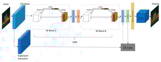
Figure 1.
Complete Network Architecture: Here, contrast and texture enhancement (CTE)-Block represents the contrast and texture enhancement block, CE Loss is the cross-entropy loss, complete architecture of SE-Block is explained in Figure 2, black arrows show the forward pass, and blue arrows show the backward error propagation.
CNNs, with the help of their convolutional filters, extract the hierarchical information from images. Shallow layers find trivial features from contexts like edges or high frequencies, while deeper layers can detect more abstract features and geometry of the objects present in the images. Each layer at each step extracts more and more salient features, to solve the task at hand efficiently. Finally, an output feature map is formed by fusing the spatial and channel information of the input data. In each layer, filters will first extract spatial features from input channels, before summing up all the information across all available output channels. Normal convolutional networks weigh up each of the output feature maps equally. Whereas, in SE-Net, each of the output channels is weighted adaptively. To put it simply, we can say that we are adding a single parameter to each channel and giving it a linear shift on the basis of how relevant each channel is. All of this is done by obtaining a global understanding of each channel by squeezing the feature maps to a single numeric value using global average pooling (GAP). This results in a vector of size n, where n is equal to the number of filter channels. Then, it is fed to the two fully connected (FC) layers of the neural network, which also outputs a vector which has the same size as the input. This n-dimensional vector can now be used to scale each original output channel based on its importance.
The complete architecture of one SE-block is shown in Figure 2. Inside each SE-Block, in each convolution layer the first value (C) represents the number of input feature maps, the second value represents the kernel size, and the third value represents the number of output channels. The dotted arrows represent the identity mapping, and r is the reduction ratio, which is the same for every block. To be concise, each SE-Block consists of a squeezing operation that extracts all the sensitive information from the feature maps, and an excitation operation that recalibrates the importance of each feature map by calculating the channel wise dependencies. We only want to capture the most salient features for the argmax classification, to produce the best results, as described earlier. Therefore, we used SE-Block to explicitly redesign the relationship between the feature maps, in such a way that the output feature maps contain as much contextual information as possible. After each SE-Block, we used batch normalization (BN), followed by a ReLu activation function. We used BN before ReLu to increase the stabilization and to accelerate the training of our network as explained in [50].
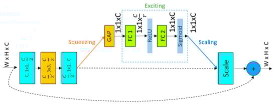
Figure 2.
Inside SE-Block. In first three convolutional blocks, first value represents the number of input feature maps, the second value represents the kernel size, and the third value represents the number of output channels. The dashed arrows represent the identity mapping. GAP, FC1, FC2 and r represent global average pooling, two densely connected layers and reduction ratio respectively.
3.4. K-Means Clustering
We used K-means as a tool to remove noise from the final segmented image. After we obtained the final segmented image, there might have still been some unwanted regions or noise present in the results, so we removed it via the K-means algorithm as in [25].
For the K-means algorithm to work, we need to specify the number of clusters (K) we want in our output image. Different algorithms have been developed to find the number of suitable clusters (K) from raw images like in [51,52,53]. In our case, because of the unsupervised scenario, we do not know in advance how many segmented regions there will be in the final segmented image. So, one way to solve this problem is to count the number of disjointed segmented regions in the final segmented image and assign that value to K. We observed that using this technique, the algorithm further improved the segmentation results. Ablation experiments which demonstrate the importance of K-means are reported in Section 6.
4. Network Training
Firstly, we enhanced the image quality using successive techniques of contrast and feature enhancement. For our algorithm neighborhood, (n × n) of size n = 7 produced best results. Then, we used the Felzenswalb algorithm [44], which assigns the same labels to pixels which have similar semantic features, to obtain pre-segmentation results. Then, we passed the enhanced image through the CNN layers for argmax classification (as explained in Section 3.3). Furthermore, we assigned the pixels which had the similar colors, textures and spatial continuity the same semantic labels. We tried to make the output of the network, i.e., argmax classification results, as close as possible to the pre-segmentation results, and the process was iterated until the desired segmented regions were obtained. In our case, iterating over an image for T = 63 times produced excellent results. We used ReLu as an activation function in our network, except at the output of the last SE-block, where we used Softmax activation to incorporate the cross-entropy loss (CE loss). For each SE-Block, we set the reduction ratio at r = 8. We backpropagated the errors and iteratively updated the gradients using a SGD optimizer, where the learning rate was set to 0.01 and the value of momentum used was β = 0.9. Finally, we used K-means clustering to further improve the segmented regions by removing the unwanted regions from the image. For the K-means clustering, the value of the K-clusters was chosen by the algorithm itself by calculating the number of unique clusters in the segmented image. We trained our network on NVIDIA GE-FORCE RTX 2080 Titan, and on average it took about 2.95 s to produce the final segmented image, including all the enhancement and refinement stages.
| Learning Algorithm: Unsupervised Semantic Segmentation |
 |
5. Results and Discussion
We evaluated our proposed algorithm on the Berkeley Segmentation Dataset (BSDS-500) [54], which is a state of the art benchmark for image segmentation and boundary detection algorithms. The segmentation results of proposed algorithm are shown in Figure 3 and Figure 4. We also compared the results of our proposed algorithm with algorithm [42], the results were compared with both variants of the algorithm [42] (i.e., using SLIC and Felzenswalb) in Figure 5 and Figure 6. It can be seen from the figures that our proposed algorithm is able to produce meaningful segmented regions from the raw unprocessed input images. The boundaries of the objects are sharp and correctly defined and one object is assigned with one semantic label. Moreover, because of the FCN based architecture of our network, it can process images of multiple resolution without any modification at all. Algorithms that need a fixed size input and perform image warping, cropping and resizing, introduce severe geometrical deformation in the images, which is not suitable for some applications.
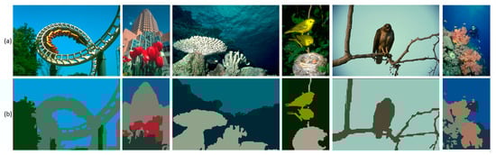
Figure 3.
Segmentation results. From top to bottom: (a) Original images, (b) segmentation results of proposed algorithm.
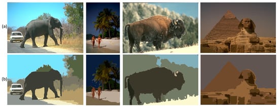
Figure 4.
Segmentation results. From top to bottom: (a) Original images, (b) segmentation results of proposed algorithm.
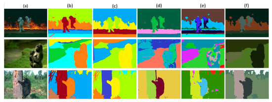
Figure 5.
From left to right: (a) original images (b) and (c) ground truths provided by different annotators, (d) and (e) segmentation results of the algorithm of [42] with Felzenswalb and SLIC, respectively, (f) segmentation results of proposed algorithm.
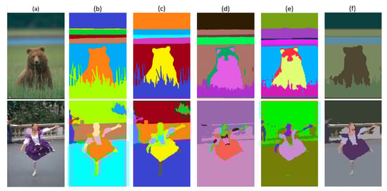
Figure 6.
From left to right: (a) Original images, (b) and (c) ground truths provided by different annotators, (d) and (e) segmentation results of algorithm of [42] with Felzenswalb and SLIC respectively, (f) segmentation results of proposed algorithm.
5.1. Performance Assessment
To provide a basis of comparison for the performance of our SEEK algorithm, we evaluated the performance of our network on multiple benchmark criteria. In this section, we present the details of our evaluation framework. The BSDS500 dataset contains 200 test, 200 train and 100 validation images. It is being used as a benchmark dataset for several segmentation algorithms like [55,56,57]. The dataset contains very distinct landscapes and sceneries. It also has multiple resolution images, which makes it ideal for testing our algorithm. The corresponding ground truth (GT) segmentation maps of all the images are labelled by different annotators [24,55,58]. A few examples of the multiple annotations for one image, are shown in Figure 5 and Figure 6, along with the original images and segmentation results. We evaluate all the images on various metrics one by one. For each image, when corresponding segmentation results are compared with the multiple GT segmentation maps, we obtain multiple values for each metric. We take the mean of those values and retain those mean values as evaluation results.
5.1.1. Variation of Information
Originally, variation of information (VI) was introduced for the general clustering evaluation [59]. However, it is also being used in the evaluation of segmentation tasks by a lot of benchmarks [23,24]. VI works by measuring the distance between the two segmentations (predicted, ground truth) in terms of their average conditional entropy. VI is defined in Equation (1) as:
If S represents the predicted segmentation result and M denotes the GT label, then H(S) and H(M) are the conditional entropies of the respective inputs, where I represents the mutual information between these two segmentations [60]. Here, a perfect score for this metric would be zero. We can say that, except VI, the larger value is better for the metrics. For VI however, smaller is better. The same conclusion can also be drawn from Table 1, where we can see that our proposed algorithm has the lowest VI.

Table 1.
The improvement in mean IoU for different networks.
5.1.2. Precision and Recall
In the context of segmentation, recall means the ability of a model to label all the pixels of the given instance to some class, and precision can be thought of as a network’s ability to only give specific labels to the pixels that actually belong to a class of interest. Precision can be defined as:
Recall is defined in Equation (3):
Here true positives (TP) are the number of pixels that are labelled as positive and are actually also from the positive class. True negatives (TN) are the number of pixels that were labelled as negative and also belong to the negative class. False positives (FP) are the number of pixels which belong to the negative class, but were wrongly predicted as positive by the algorithm. False negatives (FN) are the number of pixels that were wrongly predicted as negative but actually belong to the positive class.
While recall represents the ability of a network to find all the relevant data points in a given instance, precision represents the proportion of the pixels that our model says are relevant and are actually relevant. Whether we want high recall or high precision depends upon the application of our model. In the case of unsupervised segmentation, we can see that we need a high recall so that we don’t miss any object in the segmented output. Table 1 gives us a comparison of the performance of different setups of our model, along with other algorithms. We can see from Table 1 that all the unsupervised algorithms have a very high recall.
5.1.3. Jaccard Index
The Jaccard index, also known as intersection over union (IoU), is one of the most widely used metrics in semantic segmentation. This metric is used for gauging the similarity and diversity of input samples. It is used in the evaluation of a lot of state of the art segmentation benchmarks [61,62,63,64]. If we represent our segmentation result by S, and the GT labels which are represented by M, then it is defined as:
Table 1: Evaluation Benchmarks on BSDS500. Here, SLIC* and Felzenswalb* represent the results of variants of the algorithm [42]. SE represents our base CNN architecture; (SE+CTE) shows the results of our model with only CTE-Block as pre-processing unit, (SE + K) represents the results with only K-means block as post-processing unit. Last row, SEEK, shows the results on our complete architecture with all pre- and post-processing blocks included.
5.1.4. Dice Coefficient
The dice coefficient, also referred to as the F1-score, is also a popular metric, along with the Jaccard index. The dice coefficient is somewhat similar to the Jaccard index. Both of them are positively correlated. Even though these two metrics are functionally equivalent, their difference emerges when taking the average score over a set of inferences. It is given by the equation:
The Jaccard index generally penalizes mistakes made by networks more than the F1-score. It can have a squaring effect on the errors relative to the F1-score. We can say that the F1-score tends to measure the average performance, while the Jaccard index (IoU) measures the worst case performance of the network. From Table 1, one can also see that the F1-score is always higher than the Jaccard index (IoU) for all the setups, which also proves the above statement.
6. Ablation Study
We also performed some ablation experiments to better explain our work and to demonstrate the importance of each block in the proposed network architecture. We performed all ablation experiments on the BSDS-500 dataset using the same GPUs, while keeping the backbone architecture (SE-ResNet) the same. We demonstrated the effect of inclusion and exclusion of the contrast and texture enhancement block (CTE-block) and the K-means clustering block.
Form Table 1 (third row), we can see that if we remove the contrast and texture enhancement block, then all the metrics are affected. From Figure 7, we can also see that one of the effects of this block is that some parts of the objects get wrongly segmented as BG, e.g., tail of the insect, basket and hand of the woman, antlers of the deer, and the person with parachute. Moreover, the boundaries of the segmented regions are not sharp. So, we can say that contrast and texture enhancement block makes the architecture more robust and immune to weak noises in the image.
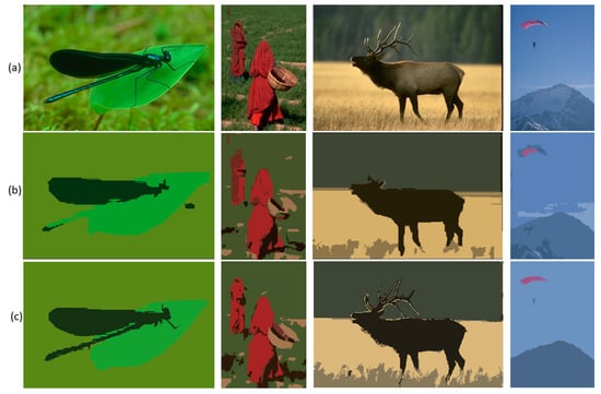
Figure 7.
Comparison of segmentation results with and without contrast and texture enhancement (CTE). From top to bottom: (a) Original images, (b) w/o CTE-block some parts of the objects get wrongly classified as the background (e.g., insect’s tail, woman’s hand and basket, deer’s antlers, and man with parachute), moreover, the boundaries of the segmented regions are not sharp, (c) w CTE-block, the insect’s tail, deer’s antlers and man are properly segmented.
The motive behind adding the K-means block in the algorithm is to further improve the segmentation results by removing the unwanted and wrongly segmented regions from the output of our neural network. The results are shown in Figure 8 visually, and quantitatively in Table 1 (fourth row). It is fairly clear from the results that, by using K-means as a segmentation refinement step, we get better segmentation results.
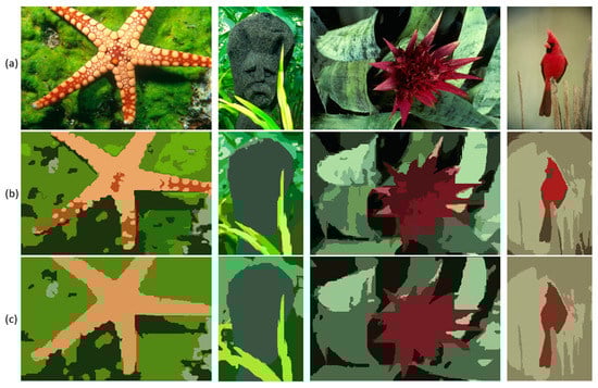
Figure 8.
Comparison of segmentation results with and without K-means post-processing. From top to bottom: (a) Original images, (b) w/o K-means refinement, a lot of unwanted segment regions are formed (e.g., starfish has dark colored spots, flower is also segmented into two segments, and the same with the bird, as it has two different colored segments), (c) w K-means refinement step, one object is given only one label.
7. Conclusions
This paper introduces a deep learning based framework for unaided semantic segmentation. The proposed architecture does not need any training data or prior ground truth. It learns to segment the input image by iterating over it repeatedly and assigning specific cluster labels to similar pixels in conjunction, while also updating the parameters of the convolution filters to get even better and more meaningful segmented regions. Moreover, image enhancement and segmentation refinement blocks of our proposed framework make our algorithm more robust and immune to various noises in the images. Based on our results, we are of the firm belief that our algorithm will be of great help in the domains of computer vision where pixel level labels are hard to obtain and also in the fields where collecting training data for sufficiently large networks is very hard to do. Moreover, because of the SE-Block backbone of our algorithm, it can take input data of any resolution. In that way, it does not produce any geometrical deformations in the images introduced by the warping, resizing and cropping of images that would be done by other algorithms. Lastly, different variants of our network can find intuitive applications in various domains of computer vision and AI.
Author Contributions
Conceptualization, T.I. and H.K.; methodology, T.I. and H.K.; software, T.I.; validation, T.I., M.U. and A.K.; formal analysis, T.I.; investigation, T.I.; resources, T.I. and H.K.; data curation, T.I.; writing—original draft preparation, T.I.; writing—review and editing, M.U. and T.I.; visualization, A.K.; supervision, H.K.; project administration, H.K.; funding acquisition, H.K. All authors have read and agreed to the published version of the manuscript.
Funding
This work was supported by the Basic Science Research Program through the National Research Foundation of Korea (NRF) funded by the Ministry of Education (NRF-2019R1A6A1A09031717 and NRF-2019R1A2C1011297).
Conflicts of Interest
The authors declare no conflict of interest.
References
- Kauanova, S.; Vorobjev, I.; James, A.P. Automated image segmentation for detecting cell spreading for metastasizing assessments of cancer development. In Proceedings of the 2017 International Conference on Advances in Computing, Communications and Informatics (ICACCI), Udupi, India, 13–16 September 2017. [Google Scholar]
- Ronneberger, O.; Fischer, P.; Brox, T. U-net: Convolutional networks for biomedical image segmentation. In International Conference on Medical Image Computing and Computer-Assisted Intervention; Springer: Berlin, Germany, 2015. [Google Scholar]
- Işın, A.; Direkoğlu, C.; Şah, M. Review of MRI-based brain tumor image segmentation using deep learning methods. Procedia Comput. Sci. 2016, 102, 317–324. [Google Scholar] [CrossRef]
- Zhou, Z.; Sodha, V.; Siddiquee, M.M.R.; Feng, R.; Tajbakhsh, N.; Gotway, M.B.; Liang, J. Models genesis: Generic autodidactic models for 3d medical image analysis. In International Conference on Medical Image Computing and Computer-Assisted Intervention; Springer: Berlin, Germany, 2019. [Google Scholar]
- Yin, J.; Mao, H.; Xie, Y. Segmentation Methods of Fruit Image and Comparative Experiments. In Proceedings of the 2008 International Conference on Computer Science and Software Engineering, Hubei, China, 12–14 December 2008. [Google Scholar]
- Lamb, N.; Chuah, M.C. A strawberry detection system using convolutional neural networks. In Proceedings of the 2018 IEEE International Conference on Big Data (Big Data), Seattle, WA, USA, 10–13 December 2018. [Google Scholar]
- Bargoti, S.; Underwood, J.P. Underwood, Image segmentation for fruit detection and yield estimation in apple orchards. J. Field Robot. 2017, 34, 1039–1060. [Google Scholar] [CrossRef]
- Chen, Y.; Lee, W.S.; Gan, H.; Peres, N.A.; Fraisse, C.W.; Zhang, Y.; He, Y. Strawberry Yield Prediction Based on a Deep Neural Network Using High-Resolution Aerial Orthoimages. Remote Sens. 2019, 11, 1584. [Google Scholar] [CrossRef]
- Tian, Y.W.; Li, C.H. Color image segmentation method based on statistical pattern recognition for plant disease diagnose [J]. J. Jilin Univ. Technol. 2004, 2, 28. [Google Scholar]
- Hofmarcher, M.; Unterthiner, T.; Arjona-Medina, J.; Klambauer, G.; Hochreiter, S.; Nessler, B. Visual scene understanding for autonomous driving using semantic segmentation. In Explainable AI: Interpreting, Explaining and Visualizing Deep Learning; Springer: Berlin, Germany, 2019; pp. 285–296. [Google Scholar]
- Fujiyoshi, H.; Hirakawa, T.; Yamashita, T. Deep learning-based image recognition for autonomous driving. IATSS Res. 2019, 43, 244–252. [Google Scholar] [CrossRef]
- Imai, T. Legal regulation of autonomous driving technology: Current conditions and issues in Japan. IATSS Res. 2019, 43, 263–267. [Google Scholar] [CrossRef]
- Leo, M.; Furnari, A.; Medioni, G.G.; Trivedi, M.; Farinella, G.M. Deep Learning for Assistive Computer Vision. In Proceedings of the Computer Vision; Springer: Berlin, Germany, 2019; pp. 3–14. [Google Scholar]
- Huang, Z.; Pan, Z.; Lei, B. Transfer Learning with Deep Convolutional Neural Network for SAR Target Classification with Limited Labeled Data. Remote Sens. 2017, 9, 907. [Google Scholar] [CrossRef]
- Lin, Z.; Ji, K.; Kang, M.; Leng, X.; Zou, H. Deep Convolutional Highway Unit Network for SAR Target Classification With Limited Labeled Training Data. IEEE Geosci. Remote Sens. Lett. 2017, 14, 1–5. [Google Scholar] [CrossRef]
- Zhao, H.; Kit, C. Integrating unsupervised and supervised word segmentation: The role of goodness measures. Inf. Sci. 2011, 181, 163–183. [Google Scholar] [CrossRef]
- Epifanio, I.; Soille, P. Morphological Texture Features for Unsupervised and Supervised Segmentations of Natural Landscapes. IEEE Trans. Geosci. Remote Sens. 2007, 45, 1074–1083. [Google Scholar] [CrossRef]
- Badrinarayanan, V.; Badrinarayanan, V.; Cipolla, R. SegNet: A Deep Convolutional Encoder-Decoder Architecture for Image Segmentation. IEEE Trans. Pattern Anal. Mach. Intell. 2017, 39, 2481–2495. [Google Scholar] [CrossRef] [PubMed]
- Chen, L.; Papandreou, G.; Kokkinos, I.; Murphy, K.; Yuille, A.L. Semantic image segmentation with deep convolutional nets and fully connected crfs. In Proceedings of the 2014 International Conference on Learning Representations, Banff, AB, Canada, 14–16 April 2014. [Google Scholar]
- Long, J.; Shelhamer, E.; Darrell, T. Fully convolutional networks for semantic segmentation. In Proceedings of the 2015 IEEE Conference on Computer Vision and Pattern Recognition (CVPR), Boston, MA, USA, 7–12 June 2015; pp. 3431–3440. [Google Scholar]
- Zheng, S.; Jayasumana, S.; Romera-Paredes, B.; Vineet, V.; Su, Z.; Du, D.; Huang, C.; Torr, P.H.S.; Shuai, Z.; Sadeep, J.; et al. Conditional Random Fields as Recurrent Neural Networks. In Proceedings of the 2015 IEEE International Conference on Computer Vision (ICCV), Boston, MA, USA, 7–12 June 2015; pp. 1529–1537. [Google Scholar]
- Pont-Tuset, J.; Barron, J.T.; Malik, J.; Marques, F.; Arbelaez, P. Multiscale Combinatorial Grouping for Image Segmentation and Object Proposal Generation. IEEE Trans. Pattern Anal. Mach. Intell. 2016, 39, 128–140. [Google Scholar] [CrossRef] [PubMed]
- Xia, X.; Kulis, B. W-net: A deep model for fully unsupervised image segmentation. arXiv 2017, arXiv:1711.08506. [Google Scholar]
- Arbelaez, P.; Maire, M.; Fowlkes, C.; Malik, J. Contour Detection and Hierarchical Image Segmentation. IEEE Trans. Pattern Anal. Mach. Intell. 2010, 33, 898–916. [Google Scholar] [CrossRef] [PubMed]
- Zheng, X.; Lei, Q.; Yao, R.; Gong, Y.; Yin, Q. Image segmentation based on adaptive K-means algorithm. EURASIP J. Image Video Process. 2018, 2018, 68. [Google Scholar] [CrossRef]
- Zhu, J.; Mao, J.; Yuille, A.L. Learning from weakly supervised data by the expectation loss svm (e-svm) algorithm. In Advances in Neural Information Processing Systems 27; NeurIPS: San Diego, CA, USA, 2014. [Google Scholar]
- Chang, F.-J.; Lin, Y.-Y.; Hsu, K.-J. Multiple structured-instance learning for semantic segmentation with uncertain training data. In Proceedings of the IEEE Conference on Computer Vision and Pattern Recognition, Columbus, OH, USA, 24–27 June 2014. [Google Scholar]
- Noh, H.; Hong, S.; Han, B. Learning Deconvolution Network for Semantic Segmentation. In Proceedings of the 2015 IEEE International Conference on Computer Vision (ICCV), Santiago, Chile, 7–13 December 2015. [Google Scholar]
- Chaurasia, A.; Culurciello, E. Linknet: Exploiting encoder representations for efficient semantic segmentation. In Proceedings of the 2017 IEEE Visual Communications and Image Processing (VCIP), St. Petersburg, FL, USA, 10–13 December 2017. [Google Scholar]
- Paszke, A.; Chaurasia, A.; Kim, S.; Culurciello, E. Enet: A Deep Neural Network Architecture for Real-Time Semantic Segmentation; Cornell University: Ithaca, NY, USA, 2016. [Google Scholar]
- Krähenbühl, P.; Koltun, V. Efficient Inference in Fully Connected Crfs with Gaussian Edge Potentials. Adv. Neural Inf. Process. Syst. 2011, 24, 109–117. [Google Scholar]
- Wei, X.; Yang, Q.; Gong, Y.; Ahuja, N.; Yang, M.H. Superpixel hierarchy. IEEE Trans. Image Process. 2018, 27, 4838–4849. [Google Scholar] [CrossRef]
- Lei, T.; Jia, X.; Liu, T.; Liu, S.; Meng, H.; Nandi, A. Adaptive Morphological Reconstruction for Seeded Image Segmentation. IEEE Trans. Image Process. 2019, 28, 5510–5523. [Google Scholar] [CrossRef]
- Bosch, M.B.; Gifford, C.; Dress, A.; Lau, C.; Skibo, J. Improved image segmentation via cost minimization of multiple hypotheses. arXiv 2018, arXiv:1802.00088. [Google Scholar]
- Fu, X.; Wang, C.-Y.; Chen, C.; Wang, C.; Kuo, C.-C.J. Robust Image Segmentation Using Contour-Guided Color Palettes. In Proceedings of the 2015 IEEE International Conference on Computer Vision (ICCV), Aracuano Park, Chile, 11–18 December 2015. [Google Scholar]
- Xu, Y.; Carlinet, E.; Géraud, T.; Najman, L. Hierarchical Segmentation Using Tree-Based Shape Spaces. IEEE Trans. Pattern Anal. Mach. Intell. 2017, 39, 457–469. [Google Scholar] [CrossRef]
- Xu, L.; Bennamoun, M.; Boussaid, F.; An, S.; Sohel, F. An Improved Approach to Weakly Supervised Semantic Segmentation. In Proceedings of the 2019 IEEE International Conference on Acoustics, Speech and Signal Processing (ICASSP), Brighton, UK, 12–17 May 2019. [Google Scholar]
- Wang, W.; Xiang, D.; Ban, Y.; Zhang, J.; Wan, J. Superpixel-Based Segmentation of Polarimetric SAR Images through Two-Stage Merging. Remote Sens. 2019, 11, 402. [Google Scholar] [CrossRef]
- Soltaninejad, M.; Yang, G.; Lambrou, T.; Allinson, N.; Jones, T.L.; Barrick, T.R.; Howe, F.; Ye, X. Automated brain tumour detection and segmentation using superpixel-based extremely randomized trees in FLAIR MRI. Int. J. Comput. Assist. Radiol. Surg. 2016, 12, 183–203. [Google Scholar] [CrossRef] [PubMed]
- Daoud, M.I.; Atallah, A.A.; Awwad, F.; Al-Najjar, M.; Alazrai, R. Automatic superpixel-based segmentation method for breast ultrasound images. Expert Syst. Appl. 2019, 121, 78–96. [Google Scholar] [CrossRef]
- Zhang, Y.; Yang, L.; Zheng, H.; Liang, P.; Mangold, C.; Loreto, R.G.; Hughes, D.P.; Chen, D.Z. SPDA: Superpixel-based data augmentation for biomedical image segmentation. arXiv 2019, arXiv:1903.00035. [Google Scholar]
- Kanezaki, A. Unsupervised image segmentation by backpropagation. In Proceedings of the 2018 IEEE International Conference on Acoustics, Speech and Signal Processing (ICASSP), Calgary, AB, Canada, 15–20 April 2018. [Google Scholar]
- Achanta, R.; Shaji, A.; Smith, K.; Lucchi, A.; Fua, P.; Süsstrunk, S. SLIC Superpixels Compared to State-of-the-Art Superpixel Methods. IEEE Trans. Pattern Anal. Mach. Intell. 2012, 34, 2274–2282. [Google Scholar] [CrossRef]
- Felzenszwalb, P.F.; Huttenlocher, D.P. Efficient Graph-Based Image Segmentation. Int. J. Comput. Vis. 2004, 59, 167–181. [Google Scholar] [CrossRef]
- Weiss, Y. Segmentation using eigenvectors: A unifying view. In Proceedings of the Seventh IEEE International Conference on Computer Vision, Kerkrya, Greece, 20–27 September 1999. [Google Scholar]
- Comaniciu, D.; Meer, P. Robust analysis of feature spaces: Color image segmentation. In Proceedings of the IEEE Computer Society Conference on Computer Vision and Pattern Recognition, San Juan, PR, USA, 17–19 June 1997. [Google Scholar]
- Vergés, L.J. Color. Constancy and Image Segmentation Techniques for Applications to Mobile Robotics. Ph.D. Thesis, Universitat Politècnica de Catalunya, Barcelona, Spain, 2005. [Google Scholar]
- Hu, J.; Shen, L.; Sun, G. Squeeze-and-excitation networks. In Proceedings of the IEEE Conference on Computer Vision and Pattern Recognition, Salt Lake City, UT, USA, 18–23 June 2018. [Google Scholar]
- He, K.; Zhang, X.; Ren, S.; Sun, J. Deep residual learning for image recognition. In Proceedings of the IEEE Conference on Computer Vision and Pattern Recognition. arXiv 2016, arXiv:1512.03385. [Google Scholar]
- Galloway, A.; Golubeva, A.; Tanay, T.; Moussa, M.; Taylor, G.W. Batch Normalization is a Cause of Adversarial Vulnerability. In Proceedings of the ICML Workshop on Identifying and Understanding Deep Learning Phenomena, Long Beach, CA, USA, 15 June 2019. [Google Scholar]
- Kaur, G.; Rani, J. MRI Brain Tumor Segmentation Methods—A Review; Infinite Study: Conshohocken, PA, USA, 2016. [Google Scholar]
- Yedla, M.; Pathakota, S.R.; Srinivasa, T.M. Enhancing K-means clustering algorithm with improved initial center. Int. J. Comp. Sci. Inf. Technol. 2010, 1, 121–125. [Google Scholar]
- Nazeer, K.A.; Sebastian, M. Improving the Accuracy and Efficiency of the k-means Clustering Algorithm. In Proceedings of the World Congress on Engineering; Association of Engineers: London, UK, 2009. [Google Scholar]
- Martín, D.; Fowlkes, C.; Tal, D.; Malik, J. A database of human segmented natural images and its application to evaluating segmentation algorithms and measuring ecological statistics. In Proceedings of the Proceedings Eighth IEEE International Conference on Computer Vision. ICCV 2001, Vancouver, BC, Canada, 7–14 July 2001. [Google Scholar]
- Wang, G.; De Baets, B. Superpixel Segmentation Based on Anisotropic Edge Strength. J. Imaging 2019, 5, 57. [Google Scholar] [CrossRef]
- Gupta, A.K.; Seal, A.; Khanna, P. Divergence based SLIC. Electron. Lett. 2019, 55, 783–785. [Google Scholar] [CrossRef]
- He, J.; Zhang, S.; Yang, M.; Shan, Y.; Huang, T. Bi-Directional Cascade Network for Perceptual Edge Detection. In Proceedings of the 2019 IEEE/CVF Conference on Computer Vision and Pattern Recognition (CVPR), Long Beach, CA, USA, 15–20 June 2019. [Google Scholar]
- Donoser, M.; Schmalstieg, D. Discrete-Continuous Gradient Orientation Estimation for Faster Image Segmentation. In Proceedings of the 2014 IEEE Conference on Computer Vision and Pattern Recognition, Columbus, OH, USA, 23–28 June 2014. [Google Scholar]
- Meila, M. Comparing Clusterings by the Variation of Information. In Learning Theory and Kernel Machines; Springer: Berlin, Germany, 2003; Volume 2777, pp. 173–187. [Google Scholar]
- Meilǎ, M. Comparing clusterings: An axiomatic view. In Proceedings of the 22nd International Conference on Machine Learning, Bonn, Germany, 7–11 August 2015. [Google Scholar]
- Cordts, M.; Omran, M.; Ramos, S.; Rehfeld, T.; Enzweiler, M.; Benenson, R.; Franke, U.; Roth, S.; Schiele, B. The Cityscapes Dataset for Semantic Urban Scene Understanding. In Proceedings of the 2016 IEEE Conference on Computer Vision and Pattern Recognition (CVPR), Las Vegas, NV, USA, 27–30 June 2016. [Google Scholar]
- Peng, C.; Zhang, X.; Yu, G.; Luo, G.; Sun, J. Large Kernel Matters—Improve Semantic Segmentation by Global Convolutional Network. In Proceedings of the 2017 IEEE Conference on Computer Vision and Pattern Recognition (CVPR), Honolulu, HI, USA, 21–26 July 2017. [Google Scholar]
- Lin, G.; Milan, A.; Shen, C.; Reid, I.D. RefineNet: Multi-path Refinement Networks for High-Resolution Semantic Segmentation. In Proceedings of the 2017 IEEE Conference on Computer Vision and Pattern Recognition (CVPR), Honolulu, HI, USA, 21–26 July 2017. [Google Scholar]
- Zhao, H.; Shi, J.; Qi, X.; Wang, X.; Jia, J. Pyramid Scene Parsing Network. In Proceedings of the 2017 IEEE Conference on Computer Vision and Pattern Recognition (CVPR), Honolulu, HI, USA, 21–26 July 2017. [Google Scholar]
© 2020 by the authors. Licensee MDPI, Basel, Switzerland. This article is an open access article distributed under the terms and conditions of the Creative Commons Attribution (CC BY) license (http://creativecommons.org/licenses/by/4.0/).