Abstract
The present paper deals with neural algorithms to learn the singular value decomposition (SVD) of data matrices. The neural algorithms utilized in the present research endeavor were developed by Helmke and Moore (HM) and appear under the form of two continuous-time differential equations over the special orthogonal group of matrices. The purpose of the present paper is to develop and compare different numerical schemes, under the form of two alternating learning rules, to learn the singular value decomposition of large matrices on the basis of the HM learning paradigm. The numerical schemes developed here are both first-order (Euler-like) and second-order (Runge-like). Moreover, a reduced Euler scheme is presented that consists of a single learning rule for one of the factors involved in the SVD. Numerical experiments performed to estimate the optical-flow (which is a component of modern IoT technologies) in real-world video sequences illustrate the features of the novel learning schemes.
1. Introduction
The computation of the singular value decomposition (SVD) of a non-square matrix [1,2,3] plays a key role in a number of applications (see, for instance, [4,5,6,7,8,9,10,11,12,13]); among them, it is worth citing applications in automatic control [14], digital circuit design [15], time-series prediction [16], and image processing [17,18]. Efforts have been devoted to achieving the computation of the SVD of matrices in the artificial neural networks community [19,20,21].
The neural algorithms utilized in the present research work to learn an SVD of a data matrix were developed by Helmke and Moore (HM) in [1]. An HM learning rule appeared under the form of two continuous-time differential equations over the special orthogonal group of matrices. The purpose of the present research is to develop and compare different numerical schemes, under the form of two alternating learning equations, to learn the SVD of large matrices on the basis of the HM learning paradigm. The numerical schemes developed here are both first-order (Euler-like) and second-order (Runge-like). Moreover, a reduced Euler scheme will be presented that consists of a single learning equation for one of the factors involved in the SVD.
The developed methods to learn an SVD of a data matrix are applied to optical-flow estimation. Optical flow estimation is a well-known image-processing operation that allows estimating the motion of portions of an image over a video sequence and has found widespread applications (see, for instance, [22,23,24,25,26,27,28,29]). Optical flow is closely related to motion estimation [30]. Optical flow refers to the change of structured light in an image and captures such change through a velocity vector field. Most of the optical-flow estimation algorithms used in video encoding belong to either the class of block matching algorithms (BMAs) or to the class of pixel recursive algorithms (PRAs) [31].
Optical flow estimation algorithms are essential components in a number of complex Internet of Things (IoT) technologies, as testified by several existing applications, such as intelligent fall detection [32,33], mobile robotics [34], intelligent flight monitoring [35], mobile object tracing [36], automated surveillance [37], smart healthcare [38], solar energy forecasting [39], and in IoT-based analytics in urban space, shops, and retail stores to inform policy makers, shop owners, and the general public about how they interact with the physical space [40]. See also the interesting discussion in [41].
The majority of the current optical-flow estimation methods rely on a block-matching algorithm. The BMA methods are based on the concept of template-matching: it is supposed that a single block in a time-frame has moved solidly to another location in the next time-frame, so the image-block is regarded as a template to be looked for in the subsequent frame. The BMA methods try to evaluate the motion of a block by reducing the number of search locations in the search range and/or by reducing the number of computations at each search location. These algorithms are either ad hoc or are based on the assumption that the error increases monotonically from the best-match location. However, typically, the error surface may exhibit local minima, and the majority of the BMAs get trapped in one of the local minima depending on the starting point and on the search direction. Furthermore, the matching algorithms aim at finding the best match with respect to some selected mismatch (error) measure, but the best match may not represent the true motion [42].
Conversely, standard PRAs try to estimate the motion at each pixel. In the method for optical-flow estimation considered here, based on the paper [42], a methodology similar to the PRA is employed, except that the algorithm operates on a pixel-block basis and finds a single motion-vector for each block. In order to make the method robust in a noisy environment, a total least squares (TLS) estimation approach is invoked. Total least squares may be implemented numerically through singular value decomposition (SVD). Other matrix decomposition techniques, such as eigenvalue decomposition, have been used in the scientific literature [43].
Throughout the paper, we use the following notation: symbol denotes a pseudo-identity matrix of size and , while symbol denotes a all-zero matrix, symbol denotes the transpose of the matrix X, and symbol denotes the trace of the square matrix X, i.e., the sum of its in-diagonal entries. The special orthogonal group is denoted and defined by . For details on this Lie group, see, e.g., [44]. Furthermore, the Frobenius norm of a matrix is denoted and defined by .
2. Helmke–Moore Learning and Advanced Numerical Methods
In the present section, we recall some essential details about the Helmke and Moore (HM) learning algorithm from [1,45]. Moreover, we survey a first-order and two second-order numerical methods to implement a learning paradigm formulated as an initial value problem (IVP, also termed the Cauchy problem) and propose numerical schemes to extend these methods to Riemannian manifolds, of which Lie groups are instances.
There exists a large variety of numerical methods to solve initial value problems. In order to limit the computational burden of the learning rules considered in this paper, we considered a Euler method, a Heun method, and a Runge method (also known as the Runge–Kutta method of the second order). These methods were developed to solve initial values problems over the Euclidean space , although they can be adapted to solve initial value problems over smooth manifolds or Lie groups, as the group .
2.1. An HM-Type Neural SVD Learning Algorithm
Denoting as a matrix whose SVD is to be computed and as the rank of Z, its singular value decomposition may be written , where and are (special) orthogonal matrices and D is a pseudo-diagonal matrix that has all-zero values except for the first r diagonal entries, termed singular values. It is easily checked that the columns of U coincide with the eigenvectors of the product , while V contains the eigenvectors of the self-product , with the same eigenvalues.
The Helmke–Moore algorithm is utilized for training, in an unsupervised way, an artificial neural network to learn an SVD of a given rectangular matrix. The HM dynamics arises from the maximization of a specific criterion defined as:
where is a weighting kernel and we assumed that . The dynamical system, derived as a Riemannian gradient flow on , reads:
where an over-dot denotes derivation with respect to the time parameter. The weighting matrix W has the structure , where must be diagonal with unequal entries on the main diagonal [45].
Since the matrix A has size , the matrix Z has size , and the matrix B has size , then the product matrix H has size .
Whereas the continuous-time versions of the learning algorithms leave the orthogonal group invariant, this is not true for their discrete-time counterparts, which are obtained by employing a numerical integration scheme, unless a suitable integration method is put into effect. In the present case, we may employ a convenient Lie integration method drawn from a manifold-calculus-based integration theory (see, e.g., the contribution [46] and previous reviews in [47,48,49]).
2.2. Euler Method in and Its Extension to
Consider the following initial value problem:
with being a regular function and with the initial condition . Whenever a closed-form solution to the IVP (3) is out of reach, the simplest numerical scheme to approximate numerically its solution is the forward Euler method described by the iterative rule:
with known from the initial condition. As a reference for this method and those invoked in the continuation of the paper, readers might refer to [50]. The constant denotes an integration stepsize and represents the time lapse between each time-node and the next. The key idea behind the above forward Euler method is to estimate the value by the slope of the vector field at the present node through a linear interpolation across the time lapse h. This Euler method is asymmetric: it makes use only of the value of the vector field f computed in the leftmost point of the interval . The right-hand side of the expression (4) coincides with the zeroth and the first terms of the Taylor series expansion of the function f. The residue owing to truncation (also termed “truncation error”) is of type ; therefore, this method is of order one.
A learning problem on the special orthogonal group is described by the IVP:
with the initial condition .
Let us recall that a smooth manifold may be endowed with a manifold exponential map and by a parallel transport operator:
- Manifold exponential: The exponential map derived from the geodesic associated with the connection is denoted by . Given and , the exponential of v at a point x is denoted as . On a Euclidean manifold , ; therefore, an exponential map may be thought of as a generalization of “vector addition” to a curved space.
- Parallel transport along geodesics: The parallel transport map is denoted by . Given two points , parallel transport from x to y is denoted as . Parallel transport moves a tangent vector between two points along their connecting geodesic arc. Given and , the parallel transport of a vector v from a point x to a point y is denoted by . Parallel transport does not change the length of a transported vector, namely it is an isometry; moreover, parallel transport does not alter the angle between transported vectors, namely, given and , it holds that , i.e., we say that parallel transport is a conformal map. Formally, on a Euclidean manifold , ; therefore, a vector transport may be thought of as a generalization of the familiar geometric notion of the “rigid translation” of vectors to a curved space.
In the case of a special orthogonal group endowed with its canonical metric (inherited by the Euclidean metric), these maps read:
where , , “Exp” denotes a matrix exponential (implemented, for example, by the function expm in MATLAB), denotes a matrix square-root (implemented, for example, by the function sqrtm in MATLAB). Let us recall that a matrix may be rewritten as , with skew-symmetric and, therefore, that the following simplified expression for the exponential map may be used:
A rule of thumb to extend the forward Euler method to smooth manifolds is that the sum between a variable representing a point and a vector field at that point needs to be replaced by the exponential map applied to the point and to the vector field at that point. As a result, a Euler method on a manifold may be expressed as:
with known from the initial condition. Likewise, the original forward Euler method, the method (8), estimates the value of the solution at the temporal node , namely , as the value of the solution at the node interpolated by the short geodesic arc departing from the current point toward the direction indicated by the vector field .
2.3. Heun and Runge Methods in and Their Extension to
The following methods are second-order numerical schemes that may be adopted to solve the Cauchy problem (3).
Heun’s method reads:
where denotes again a stepsize (or time lapse between two adjacent time nodes). It is worth summarizing an interpretation of the equations that describe the Heun method: The quantity represents an estimation of the value of the vector field f at the leftmost point of the time lapse , while the quantity represents an estimation of the value of the vector field f at the rightmost point of the time lapse . Both and are estimations, in that the expression for the quantity uses the value that is an estimation of the solution of the Cauchy problem obtained in the previous iteration, while the expression for utilizes an estimation of , indicated by , based on a linear interpolation from in the direction . The actual estimation of the solution at is obtained as a linear interpolation in a direction computed as the arithmetic average between the directions and .
Runge’s method (often denoted as “RK2”) is simpler than Heun’s, although presenting the same precision order, and is expressed as:
The quantity represents again an estimation of the value of the vector field f at the leftmost point of the time lapse , while the quantity represents an estimate of the value of the vector field f at the midpoint of the time lapse . Both and are estimations, rather than being exact evaluations. In particular, the expression for utilizes an estimation of the exact solution to the Cauchy problem, denoted by , based on a linear interpolation from in the direction extended only to half of a whole step. The actual estimation of the solution at is obtained as a linear interpolation, from in a direction extended to a whole step.
The above second-order numerical methods may be extended to a smooth manifold by recalling two simple rules-of-thumb:
- The sum between a variable representing a point on a manifold and a vector field at that point are replaced by the exponential map applied to the point and to the vector field at that point.
- The sum between two tangent vectors belonging to two different tangent spaces may be carried out only upon transporting one of the vectors to the tangent space where the other vector lives by means of parallel transport.
By applying the above rules, it is possible to extend the Heun method and the Runge method from the Euclidean space to the manifold .
Heun’s method on may be expressed as:
The above extension of the original Heun method was derived by following faithfully Heun’s concept and by replacing the linear operations with manifold operations. In particular, notice that the mean direction between and cannot be calculated as because and belong to different tangent spaces.
Runge’s method on may be expressed as:
The interpretation of the equations that constitute Runge’s method on the manifold is completely faithful to the original method.
In the following subsection, the forward Euler method, the Heun method, and the Runge method are applied to solve the HM learning system of IVPs (2). This application leads to facing at least two challenges: (1) the HM system is made of two differential equations, which entails the application of each numerical method twice; this gives rise to a non-univocality in the extension of the equations, which will then be presented in different versions; (2) the curved space may be treated as a smooth Riemannian manifold and as a Lie group; this gives rise to two different ways to design numerical methods, which will be explored and discussed in the following, even by the help of preliminary numerical tests.
2.4. Application of the Euler, Heun, and Runge Method to Solving an HM System
The HM-type learning system to solve is formed by two coupled neural learning equations, namely:
where the skew-symmetrization operator has been introduced and where the initial conditions and have been fixed.
In the following, we shall outline three different classes of numerical methods to tackle the learning problem (13), namely the (forward) Euler class, the (explicit second-order) Heun method, and the (explicit) Runge method (a second-order instance from the general class of Runge–Kutta methods). For the sake of notation compactness, in the following, we shall make use of the twin vector fields:
The numerical schemes adopted in this study are first- and second-order explicit. Implicit methods are overly complex, as they require solving a non-linear problem at every iteration (the computations involved in the implicit methods may be as complex as the problem they were designed to solve). Higher order formulations (such as the fourth-order Runge–Kutta method) are often inappropriate in optimization, because they were designed to provide a highly accurate estimation of the solution to an initial value problem at every step, while in optimization, such accuracy would be out of the scope as the only step that needs accuracy is the final optimization goal.
2.4.1. Forward Euler Method
The Euler method on outlined in Section 2.2, applied to solve an HM learning system, may be expressed as:
with and being two different learning stepsizes.
2.4.2. Explicit Second-Order Heun Method
The Heun method outlined in Section 2.3, applied to an HM learning problem on , as a manifold, may be expressed as:
It is interesting to observe that the same numerical learning algorithm may be recast in a number of slightly different ways by operating some tiny variations on the equations. An alternative version to the original Heun, Version 1 (16) is:
where the differences have been highlighted. Notice that both versions are explicit numerical schemes.
From a computational burden viewpoint, it is important to underline that the above numerical algorithms require the repeated calculation of parallel transport that contributes non-negligibly to increasing the computational complexity of these methods.
As an alternative, the Heun method may be rewritten without using parallel transport by composing the partial steps in a different way over the space , namely:
The differences with the Heun method, Version 1 (16), have been highlighted. It is interesting to observe that, by swapping the order of the steps in e (), we get:
which is computationally lighter compared to the Heun method, Version 3 (18). It is immediate to verify that Version 3 of the Heun method, further modified by the above equations, will result in being computationally lighter than the versions requiring parallel transport; therefore, the Heun method considered in the following preliminary numerical test will be:
2.4.3. Explicit Second-Order Runge Method
The Runge method outlined in Section 2.3, applied to an HM learning problem on , as a manifold, may be expressed as:
The same method may be expressed in a slightly different way, namely by exchanging the order of adaptation of the variables A and B:
The last version of the HM-type learning systems is obtained by regarding the curved space as a Lie group with Lie algebra , which leads to the following numerical method:
Even this version of the numerical learning scheme does not require using the computationally intensive parallel transport. The highlighted update equations were drawn from the survey [51].
2.5. Preliminary Pyramidal Numerical Tests on the HM Learning Methods
This subsection illustrates the results of a pyramidal comparison of the above learning algorithms in order to find out which algorithm is more convenient from a computational viewpoint, for comparable learning performances. The numerical experiments concerned the computation of the SVD of random matrices Z. The numerical experiments discussed in this subsection were performed on an Intel i5-6400T 4-Core CPU, 2.2 GHz clock, 8 GB RAM machine and were coded in a MATLAB R2017b environment (we used non-parallel programming in the experiments). In the following experiments, the learning stepsizes and were set to a common value denoted by h. Moreover, we adopted the following criterion to stop the iteration based on the objective function (1):
where denotes a threshold. The size of the unknown-matrix B was set to in all experiments, and the sub-matrix explained in the Section 2.1 was set to . The size m of the matrix B took values in (these specific values would arise in the computation of the optical-flow of pixels frames, as will be shown in Section 4.2). In all experiments, the initial matrices were chosen as and . For comparison purposes, the SVD of a matrix Z was also computed by MATLAB’s SVD engine, whose output triple is denoted by . As objective measures of the quality of the learned SVD factors, we used the following figures of demerit:
where denotes an entry-wise absolute value of a matrix. Both numerical orthogonality and discrepancy between the learned SVD and the MATLAB-computed reference SVD were expected to result in being as close as possible to zero.
The results of the first experiment, which was meant to compare the performances of the Heun method in its Versions 1 and 4, are summarized in Table 1. The random matrix Z was generated entry-wise as a set of random numbers uniformly distributed in the interval . This choice corresponded to a normalized pixel luminance, and the uniform distribution was motivated by the fact that a single pixel location may in principle take any luminance value. In the low-dimensional cases, , while in the higher dimensional case, . In all cases, . The acquired runtimes showed that Version 4 was much lighter than Version 1, a phenomenon that became more apparent as the size of the matrix A increased.

Table 1.
Results of a comparison between the runtimes (in seconds) of the Heun method in its Versions 1 and 4.
A graphical comparison of the values taken by the discrepancies defined in (25) and of the learning criterion (1) during learning is displayed in Figure 1. In this case, . The discrepancy and learning curves showed that, as concerns the learning performances, no meaningful differences between the two versions of the HM-type learning algorithms could be appreciated.
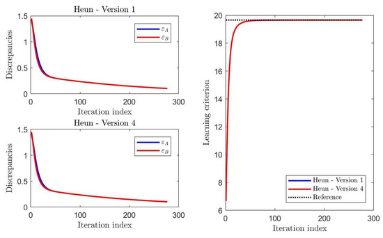
Figure 1.
Results of a comparison of the values taken by the performance indexes during learning by the Heun method in its Versions 1 and 4.
The results of this experiment entailed that the Heun method, Version 4 was the preferable version in the Heun class.
The results of the second experiment, which was meant to compare the performances of the Runge method in its Versions 1 and 3, are summarized in Table 2. In the low-dimensional cases, , while in the higher dimensional case, . In all cases, . The acquired runtimes showed that Version 3 was lighter than Version 1.
Table 2.
Results of a comparison between the runtimes (in seconds) of the Runge method in its Versions 1 and 3.
A graphical comparison of the values taken by the discrepancies and of the learning criterion during learning is displayed in the Figure 2. In this case, . The discrepancy and learning curves showed that, as concerns the learning performances, Version 1 converged only slightly more rapidly to the expected solutions.
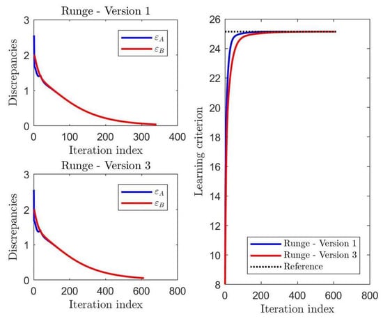
Figure 2.
Results of a comparison of the values taken by the performance indexes during learning by the Runge method in its Versions 1 and 3.
The results of this experiment entailed that the Runge method, Version 3 was the preferable version in the Runge class.
The results of the last experiment of this subsection, which was meant to compare the performances of the best Runge method and of the best Heun method to the performances of the Euler method, are summarized in Table 3. In the low-dimensional cases, , while in the higher dimensional case, . In all cases, . The acquired runtimes revealed that the Euler method was the lightest in terms of computational complexity.
Table 3.
Results of a comparison between the runtimes (in seconds) of the Heun method, Version 4, the Runge method, Version 3, and the Euler method.
A graphical comparison of the values taken by the discrepancies and of the learning criterion during learning is displayed in Figure 3. In this case, . The discrepancy and learning curves showed that, as concerns the learning performances, the Euler method-based HM learning algorithm and the Heun method-based learning algorithm converged more rapidly to the expected solutions.
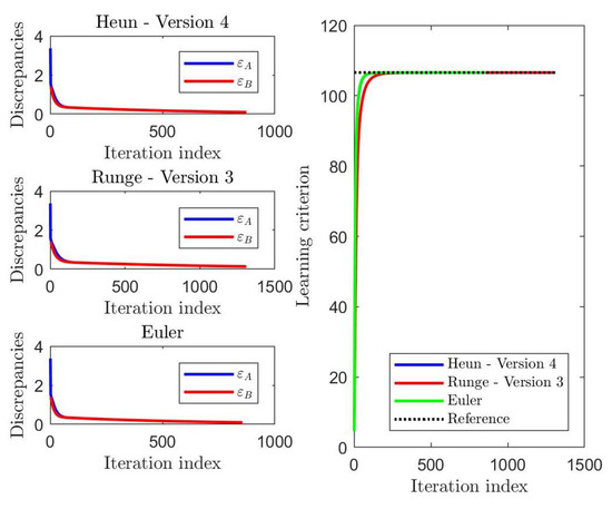
Figure 3.
Results of a comparison of the values taken by the discrepancies and the learning criterion during learning by the Heun method, Version 4, the Runge method, Version 3, and the Euler method.
A graphical comparison of the values taken by the non-orthogonality figures defined in (25) during learning is displayed in Figure 4. In this case, . The orthogonality curves showed that the Euler method-based HM was unable to keep the same numerical precision of the Heun-based and of the Runge-based HM learning algorithms, the former being a first-order method and the latter two second-order methods. However, all these algorithms kept the non-orthogonality figures at very low values and stabilized after learning completion.
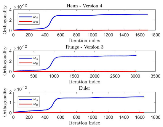
Figure 4.
Results of a comparison of the values taken by the discrepancies and the learning criterion during learning by the Heun method, Version 4, the Runge method, Version 3, and the Euler method.
The results of these three experiments revealed that the Euler method to implement a Helmke–Moore learning paradigm guaranteed an excellent trade-off between computational complexity and numerical precision.
3. Reduced Euler Method
In some applications, such as optical-flow estimation recalled in the next Section 4, only the matrix B is relevant. In view of the optical-flow application discussed in the next section, assume that B is a factor of the singular value decomposition of a data matrix Z. Notice that, in general, the matrix A has a much bigger size than the matrix B; therefore, it would be certainly convenient to express the matrix A as a function of the matrix B and to express the learning system (2) only in terms of the variable matrix B. The following arguments may be extended easily to the general case that B has different sizes.
3.1. Derivation of a Reduced Euler Method
The HM-type learning system (2) in the form (13) admits, as stable configurations, all pairs such that:
Therefore, one of these conditions may be used to express the matrix variable A in terms of the matrix variable B. In particular, the first condition, in plain form, reads:
The above equation is equivalent to . Defining , Equation (27) takes the form:
which is to be solved in A. Let us observe that the matrix K has size and that its last six rows are zero, while the matrix A has size and that its last six columns do not influence the result. Let us partition the matrices K and A as follows:
with is , is , and is . The matrix product exhibits the structure:
According to the condition (28), the product needs to result in a symmetric matrix; hence, the product needs to be symmetric, while the product needs to be zero. Since the matrix plays no role in the product , it is computationally convenient to turn down the orthogonality of the matrix A and to set , while the columns of the sub-matrix still need to be mutually orthogonal and unit-norm. Since is symmetric, let us set , where S is a symmetric matrix to be determined. To determine the unknown matrix S, let us rewrite the last equation by the ansatz , from which it follows that:
therefore:
The matrix is defined as a sub-matrix of K, which, in turn, is a function of the matrix B (and depends on the weight matrix W and on the data matrix Z). Hence, the function:
may be used to reduce the two update rules in the Euler method (15) to the single update rule:
with and with the only initial condition . Notice that the inverse matrix square root may be expressed in terms of the matrix exponential and the matrix logarithm as . The algorithm (34) will be referred to as the reduced Euler method.
3.2. Numerical Comparison of the Euler Method and Its Reduced Version
The results of a comparison of the performances of the forward Euler method (15) and of the reduced Euler method (34) to implement an HM learning paradigm are summarized in Table 4. In the low-dimensional cases, , while in the higher dimensional case, . In all cases, . The acquired runtimes showed that the reduced Euler method was way lighter than the original Euler method, a phenomenon that became more apparent as the size m of the matrix Z increased.
Table 4.
Results of a comparison between the runtimes (in seconds) for the forward Euler method and for the reduced Euler method.
A graphical comparison of the values taken by the figures of demerit defined in (25) and of the learning criterion (1) during learning is displayed in Figure 5. In this case, . The discrepancy and learning curves showed that, as concerns the learning performances, no meaningful differences between the two versions of the HM-type learning algorithms can be appreciated.
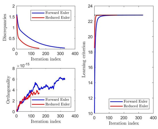
Figure 5.
Results of a comparison of the figures of demerit and of the learning criterion for the forward Euler method and for the reduced Euler method.
The results of this experiment confirmed that the reduced Euler method was both effective and efficient to implement the HM learning paradigm.
4. Experiments on Optical Flow Estimation by a Helmke–Moore Neural Learning Algorithm
In this section, we recall the notion of optical-flow estimation by a total least squares method from [42] and illustrate the behavior of the devised learning algorithm by means of numerical experiments performed on a recorded video sequence.
4.1. Optical Flow Estimation by Total Least Squares
Let us consider a gray-scale video sequence , where denotes the scalar image intensity, the pair denotes the coordinate pair of any pixel, and q denotes the frame index.
During motion, any pixel moves from frame q and position to frame at position . The fact that the pixel intensity has moved over the image support may be formally expressed by the optical-flow conservation equation, namely:
On the basis of the above conservation law, it is possible to estimate the motion of any pixel within the sequence . In fact, let us define . An application of the Taylor series expansion gives:
where and denote the partial derivatives of the image function along the vertical and the horizontal direction, respectively, and the term “residual” denotes the sum of higher order terms in the Taylor expansion of the image function and the sum of random disturbances occurring in the recording of a video sequence, while the vertical and horizontal displacements were supposed small enough for the above truncated Taylor series to represent accurately the optical-flow change. The latter hypothesis was equivalent to assuming slow motion or, equivalently, sufficiently high-rate image sampling.
As mentioned, we made the solid-block motion assumption, namely the above equation was supposed to hold true, with the same values of displacements, for a set of pixels located within the rectangular patch described by and , where integers and denote the block-size. On the basis of these considerations, it was possible to write the resolving system for any block between frames q and , that is:
where high-order terms were neglected.
By defining a displacement vector and upon defining a matrix and a vector , the above system casts into . This is an over-determined linear system of equations in two unknowns, which may be solved by the help of a total least squares technique [52].
The TLS approach to solving an over-determined system of linear equations is based on the singular value decomposition (SVD) technique [53,54]. The resulting procedure is stated in Algorithm 1.
| Algorithm 1 Total least squares based algorithm to estimate a displacement vector. |
|
It is interesting to underline that, depending on the size of each block, the data matrix Z whose SVD is to be calculated may be large sized. Moreover, for later considerations, it is important to underline that the only factor of an SVD decomposition that plays an effective role in motion estimation is V.
4.2. Numerical Experiments on Optical-Flow Learning
In order to test the capability of the HM learning paradigm in optical-flow estimation, a video was realized and saved in MP4 format. The pre-processing of the images consisted of applying a filter after the subdivision of the frames in sub-windows: every gradient matrix was examined and then the windows, which presented the null gradient, were excluded from further processing in the successive steps as they corresponded to block of pixels that were not subjected to any movement. In the post-processing, after the velocities along the x- and y-axes were calculated by using an HM learning algorithm, their norms were compared to a threshold, and all the windows that presented a velocity norm larger than the threshold were ignored in the optical-flow estimation as they were considered to correspond to noisy pixels. These filters were built to clean the image from noise created by the environment and by the camera, but they also caused a small loss of information, which could be neglected. In the experiments summarized in the present subsection, the following setting was adopted:
- The optical-flow was estimated between Frame 130 and Frame 135.
- The original colored still images drawn from the two considered frames were converted from RGB to gray scale using the luminance formula as prescribed by the recommendation ITU-R BT.601-7 [55].
- The threshold to stop iteration was set to .
- The learning stepsizes were set as .
- Given the frame size of , each frame was subdivided into windows of size , , or pixels (corresponding to 57,600 matrices of size to compute the SVD, 20,736 matrices of size to compute the SVD, and to 2304 matrices of size to compute the SVD, respectively).
- Computing platform: Intel i7-8550U 4-Core CPU, 1.8 GHz clock, 16 GB RAM. Coding platform: MATLAB R2018b.
The computational complexity related to the estimation of the optical-flow between two frames depended on the number of sub-windows and on their size; therefore, it was interesting to test the HM learning algorithms in different instances.
With reference to the HM learning paradigm, in the present application, it holds that (which depends on the size of a image’s window) while (fixed). Considering the block decomposition , with of size , the product may be simplified as , while the product may be computed as the composite matrix . Table 5 shows the results of a comparison of runtimes taken to estimate the optical-flow between two frames by the forward Euler method-based HM learning paradigm and the reduced Euler method-based algorithm.
Table 5.
Comparison of runtimes (in seconds) to compute the optical-flow between two frames by the forward Euler method and the reduced Euler method.
It is very interesting to observe how the computational complexity of the forward Euler method increased with the size of the sub-windows, while the complexity of the reduced Euler method showed an opposite trend. The time saving afforded by the reduced Euler method ranged from about for low-dimensional windows to about for high-dimensional windows.
Figure 6 illustrates the results of optical-flow estimation when the windows size was set to .
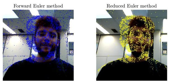
Figure 6.
Results of optical-flow estimation when the windows size was set to .
Figure 7 illustrates the results of optical-flow estimation when the windows size was set to .
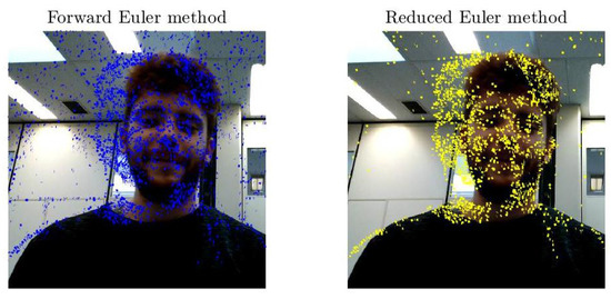
Figure 7.
Results of optical-flow estimation when the windows size was set to .
Figure 8 illustrates the results of optical-flow estimation when the windows size was taken as .
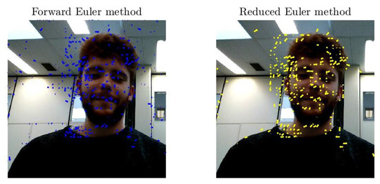
Figure 8.
Results of optical-flow estimation when the windows size was set to .
The estimation obtained through the reduced Euler method seemed cleaner and free of artifacts, which may denote a stronger robustness against noise.
5. Conclusions
The aim of this paper was to present two first-order (forward Euler and reduced Euler) and two second-order (Heun and Runge) numerical learning methods to learn the SVD of large rectangular matrices.
We recalled the Helmke–Moore learning paradigm to estimate the SVD of a given rectangular matrix, which was expressed by two coupled differential equations on the special orthogonal group. Taking the move from classical numerical calculus methods to solve ordinary differential equations, we suggested several numerical schemes to extend these classical methods to the manifold of special orthogonal matrices.
The resulting methods were tested numerically against each other in a pyramidal comparison in order to determine their merits and demerits in terms of computational complexity and effectiveness in computing the SVD. Observing that, for total least-squares-based optical-flow estimation, only one among the three SVD factors was necessary, a further reduced method was developed and tested against its non-reduced counterpart.
The conclusion of the experimental tests was that the estimation obtained through the reduced Euler method looked clean and free of artifacts, which may suggest robustness against noise and that the time saving of the reduced Euler method with respect to the forward Euler method increased noticeably when the size of the sub-windows increased.
Author Contributions
Conceptualization, S.F.; data curation, M.G.; formal analysis, S.F.; software, S.F., L.D.R., M.G., and A.S.; writing, original draft, L.D.R., M.G., and A.S.; writing, review and editing, S.F. All authors read and agreed to the published version of the manuscript.
Funding
This research received no external funding.
Conflicts of Interest
The authors declare no conflict of interest.
References
- Helmke, U.; Moore, J.B. Singular value decomposition via gradient and self-equivalent flows. Linear Algebra Appl. 1992, 169, 223–248. [Google Scholar] [CrossRef]
- Hori, G. A general framework for SVD flows and joint SVD flows. In Proceedings of the 2013 IEEE International Conference on Acoustics, Speech and Signal Processing, Vancouver, BC, Canada, 26–31 May 2013; Volume II, pp. 693–696. [Google Scholar]
- Smith, S.T. Dynamic system that perform the SVD. Syst. Control Lett. 1991, 15, 319–327. [Google Scholar] [CrossRef]
- Alter, O.; Brown, P.O.; Botstein, D. Singular value decomposition for genome-wide expression data processing and modeling. Proc. Natl. Acad. Sci. USA 2000, 97, 10101–10106. [Google Scholar] [CrossRef] [PubMed]
- Ciesielski, A.; Forbriger, T. Singular value decomposition of tidal harmonics on a rigid Earth. Geophys. Res. Abstr. 2019, 21, EGU2019-16895. [Google Scholar]
- Claudino, D.; Mayhall, N.J. Automatic partition of orbital spaces based on singular value decomposition in the context of embedding theories. J. Chem. Theory Comput. 2019, 15, 1053–1064. [Google Scholar] [CrossRef]
- Ernawan, F.; Ariatmanto, D. Image watermarking based on integer wavelet transform-singular value decomposition with variance pixels. Int. J. Electr. Comput. Eng. 2019, 9, 2185–2195. [Google Scholar] [CrossRef]
- Garcia-Pena, M.; Arciniegas-Alarcon, S.; Barbin, D. Climate data imputation using the singular value decomposition: An empirical comparison. Revista Brasileira de Meteorologia 2014, 29, 527–536. [Google Scholar]
- Hao, Z.; Cuia, Z.; Yue, S.; Wang, H. Amplitude demodulation for electrical capacitance tomography based on singular value decomposition. Rev. Sci. Instrum. 2018, 89, 074705. [Google Scholar] [CrossRef]
- Jha, A.K.; Barrett, H.H.; Frey, E.C.; Clarkson, E.; Caucci, L.; Kupinski, M.A. Singular value decomposition for photon-processing nuclear imaging systems and applications for reconstruction and computing null functions. Phys. Med. Biol. 2015, 60, 7359–7385. [Google Scholar] [CrossRef]
- Liu, Y.; Sun, Y.; Li, B. A two-stage household electricity demand estimation approach based on edge deep sparse coding. Information 2019, 10, 224. [Google Scholar] [CrossRef]
- Montesinos-López, O.A.; Montesinos-Lxoxpez, A.; Crossa, J.; Kismiantini; Ramírez-Alcaraz, J.M.; Singh, R.; Mondal, S.; Juliana, P. A singular value decomposition Bayesian multiple-trait and multiple-environment genomic model. Heredity 2019, 122, 381–401. [Google Scholar] [CrossRef] [PubMed]
- Vezyris, C.; Papoutsis-Kiachagias, E.; Giannakoglou, K. On the incremental singular value decomposition method to support unsteady adjoint—Based optimization. Numer. Methods Fluids 2019, 91, 315–331. [Google Scholar] [CrossRef]
- Moore, B.C. Principal component analysis in linear systems: Controllability, observability and model reduction. IEEE Trans. Autom. Control 1981, AC-26, 17–31. [Google Scholar] [CrossRef]
- Lu, W.-S.; Wang, H.-P.; Antoniou, A. Design of two-dimensional FIR digital filters by using the singular value decomposition. IEEE Trans. Circuits Syst. 1990, CAS-37, 35–46. [Google Scholar] [CrossRef]
- Salmeron, M.; Ortega, J.; Puntonet, C.G.; Prieto, A. Improved RAN sequential prediction using orthogonal techniques. Neurocomputing 2001, 41, 153–172. [Google Scholar] [CrossRef]
- Costa, S.; Fiori, S. Image compression using principal component neural networks. Image Vision Comput. J. 2001, 19, 649–668. [Google Scholar] [CrossRef]
- Nestares, O.; Navarro, R. Probabilistic estimation of optical-flow in multiple band-pass directional channels. Image Vision Comput. J. 2001, 19, 339–351. [Google Scholar] [CrossRef]
- Cichocki, A.; Unbehauen, R. Neural networks for computing eigenvalues and eigenvectors. Biol. Cybern. 1992, 68, 155–164. [Google Scholar] [CrossRef]
- Sanger, T.D. Two iterative algorithms for computing the singular value decomposition from input/output samples. In Advances in Neural Processing Systems; Cowan, J.D., Tesauro, G., Alspector, J., Eds.; Morgan-Kauffman Publishers: Burlington, MA, USA, 1994; Volume 6, pp. 1441–1451. [Google Scholar]
- Weingessel, A. An Analysis of Learning Algorithms in PCA and SVD Neural Networks. Ph.D. Thesis, Technical University of Wien, Wien, Austria, 1999. [Google Scholar]
- Afrashteh, N.; Inayat, S.; Mohsenvand, M.; Mohajerani, M.H. Optical-flow analysis toolbox for characterization of spatiotemporal dynamics in mesoscale optical imaging of brain activity. Neuroimage 2017, 153, 58–74. [Google Scholar] [CrossRef]
- Ayzel, G.; Heistermann, M.; Winterrath, T. Optical flow models as an open benchmark for radar-based precipitation nowcasting (rainymotion v0.1). Geosci. Model Dev. 2019, 12, 1387–1402. [Google Scholar] [CrossRef]
- Caramenti, M.; Lafortuna, C.L.; Mugellini, E.; Khaled, O.A.; Bresciani, J.-P.; Dubois, A. Matching optical-flow to motor speed in virtual reality while running on a treadmill. PLoS ONE 2018, 13, e0195781. [Google Scholar] [CrossRef] [PubMed]
- Rahmaniar, W.; Wang, W.-J.; Chen, H.-C. Real-time detection and recognition of multiple moving objects for aerial surveillance. Electronics 2019, 8, 1373. [Google Scholar] [CrossRef]
- Rosa, B.; Bordoux, V.; Nageotte, F. Combining differential kinematics and optical-flow for automatic labeling of continuum robots in minimally invasive surgery. Front. Robot. AI 2019, 6, 86. [Google Scholar] [CrossRef]
- Ruiz-Vargas, A.; Morris, S.A.; Hartley, R.H.; Arkwright, J.W. Optical flow sensor for continuous invasive measurement of blood flow velocity. J. Biophotonics 2019, 12, 201900139. [Google Scholar] [CrossRef] [PubMed]
- Vargas, J.; Quiroga, J.A.; Sorzano, C.O.S.; Estrada, J.C.; Carazo, J.M. Two-step interferometry by a regularized optical-flow algorithm. Opt. Lett. 2011, 36, 3485–3487. [Google Scholar] [CrossRef]
- Serres, J.R.; Evans, T.J.; Åkesson, S.; Duriez, O.; Shamoun-Baranes, J.; Ruffier, F.; Hedenström, A. Optic flow cues help explain altitude control over sea in freely flying gulls. J. R. Soc. Interface 2019, 16, 20190486. [Google Scholar] [CrossRef]
- Lazcano, V. An empirical study of exhaustive matching for improving motion field estimation. Information 2018, 9, 320. [Google Scholar] [CrossRef]
- Liu, L.-K.; Feig, E. A block-based gradient descent search algorithm for block motion estimation in video coding. IEEE Trans. Circuits Syst. Video Technol. 1996, 6, 419–422. [Google Scholar]
- Hsieh, Y.; Jeng, Y. Development of home intelligent fall detection IoT system based on feedback optical-flow convolutional neural network. IEEE Access 2018, 6, 6048–6057. [Google Scholar] [CrossRef]
- Núñez-Marcos, A.; Azkune, G.; Arganda-Carreras, I. Vision-based fall Detection with convolutional neural networks. Wirel. Commun. Mob. Comput. 2017, 2017, 9474806. [Google Scholar] [CrossRef]
- Toda, T.; Masuyama, G.; Umeda, K. Detecting moving objects using optical-flow with a moving stereo camera. In Proceedings of the 13th International Conference on Mobile and Ubiquitous Systems: Computing Networking and Services (MOBIQUITOUS 2016, Hiroshima, Japan, 28 November–1 December 2016; pp. 35–40. [Google Scholar]
- Hou, Y.; Wang, J. Research on intelligent flight software robot based on internet of things. Glob. J. Technol. Optim. 2017, 8, 221. [Google Scholar] [CrossRef]
- Shi, X.; Wang, M.; Wang, G.; Huang, B.; Cai, H.; Xie, J.; Qian, C. TagAttention: Mobile object tracing without object appearance information by vision-RFID fusion. In Proceedings of the 27th IEEE International Conference on Network Protocols, Chicago, IL, USA, 7–10 October 2019; pp. 1–11. [Google Scholar]
- Zulkifley, M.A.; Samanu, N.S.; Zulkepeli, N.A.A.N.; Kadim, Z.; Woon, H.H. Kalman filter-based aggressive behaviour detection for indoor environment. In Lecture Notes in Electrical Engineering; Springer: Berlin/Heidelberg, Germany, 2016; Volume 376, pp. 829–837. [Google Scholar]
- Hussain, T.; Muhammad, K.; Khan, S.; Ullah, A.; Lee, M.Y.; Baik, S.W. Intelligent baby behavior monitoring using embedded vision in IoT for smart healthcare centers. J. Artif. Intell. Syst. 2019, 1, 110–124. [Google Scholar] [CrossRef]
- IBM Research Editorial Staff. Building Cognitive IoT Solutions Using Data Assimilation. Available online: https://www.ibm.com/blogs/research/2016/12/building-cognitive-iot-solutions-using-data-assimilation/ (accessed on 9 December 2016).
- Saquib, N. Placelet: Mobile Foot Traffic Analytics System Using Custom Optical Flow. Available online: https://medium.com/mit-media-lab/placelet-mobile-foot-traffic-analytics-system-using-custom-optical-flow-19bbebfc7cf8 (accessed on 3 March 2016).
- Patrick, M. Why Machine Vision Matters for the Internet of Things. Available online: http://iot-design-zone.com/article/knowhow/2525/why-machine-vision-matters-for-the-internet-of-things (accessed on 12 December 2019).
- Deshpande, S.G.; Hwang, J.-N. Fast motion estimation based on total least squares for video encoding. Proc. Int. Symp. Circuits Syst. 1998, 4, 114–117. [Google Scholar]
- Liu, K.; Yang, H.; Ma, B.; Du, Q. A joint optical-flow and principal component analysis approach for motion detection. In Proceedings of the 2010 IEEE International Conference on Acoustics, Speech and Signal Processing, Dallas, TX, USA, 14–19 March 2010; pp. 1178–1181. [Google Scholar]
- Fiori, S. Unsupervised neural learning on Lie groups. Int. J. Neural Syst. 2002, 12, 219–246. [Google Scholar] [CrossRef]
- Fiori, S. Singular value decomposition learning on double Stiefel manifold. Int. J. Neural Syst. 2003, 13, 155–170. [Google Scholar] [CrossRef]
- Celledoni, E.; Fiori, S. Neural learning by geometric integration of reduced ‘rigid-body’ equations. J. Comput. Appl. Math. 2004, 172, 247–269. [Google Scholar] [CrossRef]
- Fiori, S. A theory for learning by weight flow on Stiefel-Grassman manifold. Neural Comput. 2001, 13, 1625–1647. [Google Scholar] [CrossRef]
- Fiori, S. A theory for learning based on rigid bodies dynamics. IEEE Trans. Neural Netw. 2002, 13, 521–531. [Google Scholar] [CrossRef]
- Fiori, S. Fixed-point neural independent component analysis algorithms on the orthogonal group. Future Gener. Comput. Syst. 2006, 22, 430–440. [Google Scholar] [CrossRef]
- Lambert, J.D. Numerical Methods for Ordinary Differential Systems: The Initial Value Problem, 1st ed.; Wiley: Hoboken, NJ, USA, 1991; ISBN 978-0471929901. [Google Scholar]
- Celledoni, E.; Marthinsen, H.; Owren, B. An introduction to Lie group integrators—Basics, new developments and applications. J. Comput. Phys. Part B 2014, 257, 1040–1061. [Google Scholar] [CrossRef]
- Golub, G.H.; van Loan, C.F. Matrix Computations, 3rd ed.; The John Hopkins University Press: Baltimore, MD, USA, 1996. [Google Scholar]
- Kong, S.; Sun, L.; Han, C.; Guo, J. An image compression scheme in wireless multimedia sensor networks based on NMF. Information 2017, 8, 26. [Google Scholar] [CrossRef]
- Wang, D. Adjustable robust singular value decomposition: Design, analysis and application to finance. Data 2017, 2, 29. [Google Scholar] [CrossRef]
- RECOMMENDATION ITU-R BT.601-7. Studio Encoding Parameters of Digital Television for Standard 4:3 and Wide-Screen 16:9 Aspect Ratios. Version 2017. Available online: https://www.itu.int/dms_pubrec/itu-r/rec/bt/R-REC-BT.601-7-201103-I!!PDF-E.pdf (accessed on 10 February 2020).
© 2020 by the authors. Licensee MDPI, Basel, Switzerland. This article is an open access article distributed under the terms and conditions of the Creative Commons Attribution (CC BY) license (http://creativecommons.org/licenses/by/4.0/).