Article

Calibration Venus: An Interactive Camera Calibration Method Based on Search Algorithm and Pose Decomposition

1
School of Computer Science and Engineering, Central South University, Changsha 410075, China
2
Beijing Mass Transit Railway Operation Co. LTD., Beijing 100000, China
3
Yewuxuan (Beijing) Communication Technology Co. LTD., Beijing 100000, China
*
Author to whom correspondence should be addressed.
Electronics 2020, 9(12), 2170; https://doi.org/10.3390/electronics9122170
Submission received: 26 October 2020 / Revised: 18 November 2020 / Accepted: 13 December 2020 / Published: 17 December 2020
(This article belongs to the Special Issue Autonomous Vehicles Technology)

Abstract

:
Cameras are widely used in many scenes such as robot positioning and unmanned driving, in which the camera calibration is a major task in this field. The interactive camera calibration method based on a plane board is becoming popular due to its stability and handleability. However, most methods choose suggestions subjectively from a fixed pose dataset, which is error-prone and limited for different camera models. In addition, these methods do not provide clear guidelines on how to place the board in the specified pose. This paper proposes a new interactive calibration method, named ‘Calibration Venus’, including two main parts: pose search and pose decomposition. First, a pose search algorithm based on simulated annealing (SA) algorithm is proposed to select the optimal pose in the entire pose space. Second, an intuitive and easy-to-use user guidance method is designed to decompose the optimal pose into four sub-poses: translation, each rotation along X-, Y-, Z-axes. Thereby the users could follow the guide step by step to accurately complete the placement of the calibration board. Experimental results evaluated on simulated and real datasets show that the proposed method can reduce the difficulty of calibration, and improve the accuracy of calibration, as well as provide better guidance.

1. Introduction

In recent years, due to the rise of virtual reality [1] and unmanned driving [2], higher requirements have been put forward for the perception of real scenes, which has promoted the rapid development of 3D reconstruction [3,4] and photogrammetry [5] technology. Camera calibration is a necessary part of these camera-based applications, the quality of calibration largely affects the effect of subsequent procedures. The purpose of camera calibration [6,7] is to obtain the values of geometric and optical characteristics of the internal camera (hereafter internal parameters), including focal length, optical center projection position, and distortion coefficients. The estimation of internal parameters is usually based on the corresponding relationship between the feature points of the calibration object and the imaging points. The camera is usually moved with respect to the calibration object, and its function is to capture the relative pose under different conditions [8,9]. The obtained pose represents the position and orientation of the calibration object relative to the camera, which can be specified by a rotation matrix and a translation vector.
The calibration effect of different calibration images obtained by different pose combinations is quite different. Some research has been focused on this aspect. Zhang et al. [10] proposed the parallel poses causing degradation, which should be avoided. The rotation angle should not be too large, because the rotation angle increases, the feature point detection error will also increase. Xie et al. [11] studied the properties of the homography matrix describing the geometric transformation relationship between the calibration board and its imaging. They summarized that the angle parallel to the image plane should be avoided. Triggles et al. [12] related the angle to the error in focal length. He also found that the rotation angle needs to be at least 5 degrees. Sturm and Maybank [13] separated the focal length and the optical center projection position for consideration. They explored the possible singularities when using one and two calibration images of various methods. It is found that if each target orientation in the calibration set is parallel to the image plane, then the focal length cannot be determined. Rojtberg et al. [14] associated the pose and the constraints of a single parameter together. He found that improving the sampling accuracy in an image region with a strong distortion can effectively constrain the distortion coefficients. He also found that maximizing the spread angle between the image plane and calibration pattern can better constrain the focal length and the projection position of the optical center.
For most users, it is an inevitable problem about how to choose the pose in the calibration process, that is, where the calibration object should be placed. Traditional calibration methods allow people to make their own decisions. It is difficult for users to complete this work without calibration experience, and even professionals need to go through many attempts to obtain a satisfactory calibration result, and a successful calibration is difficult to be reproduced. The interactive calibration has been investigated to address these issues. Unlike traditional calibration that let the user choose the pose alone, the interactive calibration will select each target pose for users, and help users obtain these poses in the actual calibration process.
Several research works have been conducted on interactive camera calibration. Richardson et al. [15] obtained a set of 60 candidate positions by uniformly sampling in the perceptual region of the camera. When the pose selection is needed, each pose in the candidate pose set is traversed to perform a hypothetical calibration. The pose with the best hypothetical calibration effect will be selected. However, since the candidate pose is obtained by uniform sampling, the degradation, and spread angle are not considered. During the user guidance process, they use an arrow to guide the user. In the real three-dimensional world, however, this can only determine a general direction of movement. Rojtberg et al. [14] select the effective pose according to the proposed strategy to better constrain the internal parameter with maximum estimation uncertainty. He groups the internal parameters and uses different pose selection strategies. He takes the focal length and the projection position of the optical center as a group and selects the pose that can maximize the overall spread angle. The distortion coefficients are taken as a group and the pose that can improve the sampling accuracy of the most distorted region is selected. During the user guidance process, the coordinate axis of the calibration board is visualized so that the user can use it as a reference for moving. However, this method needs to detect the calibration board in real-time, which brings some delay problems.
The above-mentioned researches are the strategy-based solutions, which may cause some problems to select the desired pose from a set of predefined candidate poses when these solutions are applied to different camera models or calibration modes. In addition, the solutions also rely on users to rotate the calibration plate in space for obtaining the final pose.
To address the issues, first, a novel search framework based on the entire pose space is proposed to optimize the choice of pose. After each round of calibration, the initial solution is obtained based on the initial pose method. The search is performed in the entire pose space to minimize the value of the loss function, and the searched optimal pose is used as the next expectation pose. Second, we develop a new pose decomposition guidance method that is not based on the coordinate axis as a reference, but a lazy loading processing [16] method to reduce the delay and improve the real-time performance. The decomposition results can be regarded as the final pose after translation and rotation operations along the direction of each coordinate axis. Then the decomposed poses are projected and displayed in order, which allows users to place the calibration board in a step-by-step manner and makes the entire guidance process more intuitive, efficient, and faster.
The rest of this paper is arranged as follows: Section 2 introduces the basic theory of camera calibration; Section 3 gives the calibration process and various links of this method; Section 4 conducts the experimental evaluation in the simulated and field measurement scenarios, and Section 5 gives summarizations and future prospects.

2. Basic Theory

In many computer vision tasks that use cameras, camera calibration is undoubtedly one of the most important pre-work tasks [17]. The common method of camera calibration is to model the camera imaging process, and then estimate the camera internal parameters through data sampling. Interactive camera calibration is one of the current frontier researches in the field of camera calibration. The purpose is to design a calibration method that is user-friendly, easy to operate, stable, and effective in the calibration process. The following paper will introduce the principle of camera imaging, a classic traditional calibration method: Zhang’s calibration method [10].

2.1. Camera Imaging Principle

The camera maps a 3D point in the real world to a pixel point on a two-dimensional image. The mapping process can be described utilizing coordinate system transformation. The coordinate systems commonly used in camera imaging models are given below. Figure 1 describes the transformation between these coordinate systems.

2.1.1. Coordinate System Definition

  • World coordinate system: An absolute coordinate system used to measure the position of a camera or object.
  • Camera coordinate system: A 3D rectangular coordinate system is established with the optical center of the camera as the origin and the optical axis as the positive half-axis of the Z-axis. It is the coordinate system when the camera is standing at its angle to measure objects.
  • Projection plane coordinate system: A coordinate system established with the intersection of the camera’s optical axis and the projection plane as the origin to indicate the physical position of the pixel.
  • Image coordinate system: A two-dimensional coordinate system based on the upper left corner of the digital image as the origin.
The camera imaging process can be described by a series of coordinate system transformations, named the camera imaging model. All the transformations involved in the whole imaging process will be introduced in turn.

2.1.2. Camera Imaging Process

The imaging point Q ( u , v ) of a 3D point P w ( X w , Y w , Z w ) T in the world coordinate system is obtained as follows:
Transformed into the camera coordinate system: Firstly, we need to get the position information of the point relative to the camera, that is, its 3D coordinate P c ( X c , Y c , Z c ) T in the camera coordinate system. This is obtained by rigid body transformation. The transformation equation is shown in Equation (1). ( R , T ) is the rotation matrix and translation vector in the coordinate transformation relationship between the two spatial coordinate systems.
[ X c Y c Z c ] = [ R T ] [ X w Y w Z w ]
Transformed into the projection plane coordinate system: Then the camera projects three-dimensional points onto a two-dimensional projection plane through an imaging lens. This process can be regarded as perspective transformation, transformation equation as in Equation (2), where f refers to the focal length of the camera. As shown in Figure 2, the pinhole imaging model [18] vividly shows the transformation.
Z c [ x y 1 ] = [ f 0 0 0 f 0 0 0 1 ] [ X c Y c Z c ]
Transform into the image coordinate system. Finally, the final imaging point Q(u,v) is obtained by an affine transformation, which transforms the physical position of the imaging point into the pixel position. The transformation equation is shown in Equation (3). In the following equation, dx and dy represent the conversion ratio of pixel units to physical units in the X and Y directions, respectively. (u0,v0) is the optical center which is the projection position of the optical center on the projection plane. γ is the non-perpendicular factor between the horizontal and vertical axes which can usually be assumed to be 0.
[ u v 1 ] = [ 1 d x γ u 0 0 1 d y v 0 0 0 1 ] [ x y 1 ]
Through the above conversion relationship, the conversion from a certain three-dimensional point in the world coordinate system to a pixel point in the two-dimensional image is realized. The whole imaging process can be described by Equation (4).
[ u v 1 ] = [ 1 d x γ u 0 0 1 d y v 0 0 0 1 ] [ f 0 0 0 0 f 0 0 0 0 1 0 ] [ R T 0 1 ] [ X w Y w Z w 1 ] = [ α γ u 0 0 0 β v 0 0 0 0 1 0 ] [ R T 0 1 ] [ X w Y w Z w 1 ] = K [ R T 0 1 ] P w

2.1.3. Distortion

Because the actual lens of the camera is not ideal perspective imaging, there will be a certain degree of distortion. The lens inside the camera will cause radial distortion [19] and tangential distortion [20] due to its shape and non-parallelism with the image plane during assembly. The process can be represented by Equation (5), where r represents the Euclidean distance from the point to the origin. ( k 1 , k 2 , k 3 ) represents the radial distortion parameters. ( p 1 , p 2 ) represents the tangential distortion parameters. ( x , y ) represents the point coordinates after distortion.
{ x = x ( 1 + k 1 r 2 + k 2 r 4 + k 3 r 6 ) + 2 p 1 x y + p 2 ( r 2 + 2 x 2 ) y = y ( 1 + k 1 r 2 + k 2 r 4 + k 3 r 6 ) + p 1 ( r 2 + 2 y 2 ) + 2 p 2 x y
Parameters ( α , β , u 0 , v 0 ) and distortion coefficients ( k 1 , k 2 , k 3 , p 1 , p 2 ) are collectively called camera internal parameters, and the main purpose of camera calibration is to estimate these parameters by sampling.

2.2. Zhang’s Calibration Method

Camera calibration is the process of estimating the internal parameters of the camera, which will be used for subsequent computer vision tasks, so the quality of the camera calibration greatly affects the application effect of the camera-based scene. The following briefly introduces the classic Zhang’s calibration method [10]. The method needs to capture images of a calibration object in multiple different poses (the position and angle of the calibration object relative to the camera). The initial values of the internal parameters are calculated by the mapping relationship between the feature points and their imaging, and then the internal parameters are modified by the nonlinear optimization algorithm.

2.2.1. Calculation of Initial Value

The process of mapping the feature points on the two-dimensional plane calibration board [21,22] to the pixels on the image is regarded as homography transformation (plane-to-plane transformation). Without loss of generality, the model plane is assumed to be located at Z = 0 in the world coordinate system. Then the projection equation can be simplified as Equation (6).
Z c [ u v 1 ] = K [ r 1 r 2 T ] [ X w Y w 1 ] = H [ X w Y w 1 ]
where (r1, r2) is the first two column vectors of the rotation matrix R. H is a homography matrix.
B = K T K 1 = [ 1 α 2 γ α 2 β v 0 γ u 0 β α 2 β γ α 2 β γ 2 α 2 β 2 + 1 β 2 γ ( v 0 γ u 0 β ) α 2 β 2 v 0 β 2 v 0 γ u 0 β α 2 β γ ( v 0 γ u 0 β ) α 2 β 2 v 0 β 2 ( v 0 γ u 0 β ) 2 α 2 β 2 + v 0 2 β 2 + 1 ]
Define symmetric matrix B in Equation (7). Let b = [ B 11 B 12 B 22 B 13 B 23 B 33 ] T , where Bij is the element in row i and column j in B. Let homography matrix H = [ h 1 h 2 h 3 ] . Since the rotation matrix R has the property that the column vectors are all unit vectors and are orthogonal to each other. Two constraints in Equation (8) can be obtained, which can be expanded and combined to obtain a homogeneous linear equation system.
{ h 1 T K T K 1 h 2 = 0 h 1 T K T K 1 h 1 = h 2 T K T K 1 h 2 [ v 12 T ( v 11 v 12 ) T ] b = 0
with v i j = [ h i 1 , h j 1 , h i 1 h j 2 + h i 2 h j 1 , h i 2 h j 2 . h i 3 h j 1 + h i 1 h j 3 , h i 3 h j 2 + h i 2 h j 3 , h i 3 h j 3 ] T , where h i j is the element in row i and column j in H .
When n calibration images are observed, combining n such equations can get VB = 0, where V is a 2 n 6 matrix. When the number of images >2, the equation can calculate a solution of B. When B is solved, the Cholesky matrix factorization algorithm can be used to find K 1 .

2.2.2. Maximum Likelihood Estimation

The above calculation results are based on the ideal solution, but due to the possibility of Gaussian noise, the maximum likelihood estimation is used for optimization. The obtained solution is used as the initial value, and the L-M method [23] is used for optimization, and then the internal parameter value can be calculated from the relationship between it and the internal parameter. The optimization goal is to minimize Equation (9).
i = 1 n j = 1 m m i j m ( K , R i . T i , P j ) 2

3. Calibration Process

The traditional calibration method is generally to obtain multiple images of the calibration object in different poses, and then use them as the input of the calibration algorithm for calibration. Therefore, the calibration pose has a greater impact on the calibration effect. [10,13] all pointed out some poses that can lead to bad results. One of the main goals of interactive calibration is to help beginners avoid these bad poses. Besides, the other feature in interactive camera calibration is that the system rather than humans determines the pose of the calibration object, which frees beginners from the trouble of choosing a pose.
This paper proposes an interactive camera calibration method based on a pose search algorithm and pose decomposition method. The pose search algorithm solves the optimal pose in the entire pose space. The calibration quality under different initial solutions and different loss function quantitative evaluation factors is analyzed. A step-by-step guidance method is designed. By decomposing the desired pose and displaying it, supplemented by text and rotation direction diagram for user guidance, it greatly reduces the burden on users and makes the pose realization faster and easier.
The process of the calibration method in this paper is shown in Figure 3. Firstly, the system is started to complete the initialization of the parameters to be estimated. Then enter the module to get the next pose: (1) Initialization of pose-search-related parameters. (2) The initial pose is obtained according to the method. (3) Start the pose search until the termination condition is reached and return to the optimal pose. (4) The pose search updates the adjacent solution as the optimal solution by probability. After getting the next pose, the pose is decomposed and displayed separately. This can guide the user to complete the image acquisition of the calibration board in this pose. The new image is used to calibrate and update the system parameters. If the system converges, the estimated parameters are returned, otherwise, the next pose is calculated.

3.1. Bootstrapping

At the beginning of calibration, the system does not contain any prior information on the camera’s internal parameters. To ensure the effectiveness of the initial pose, we adopted the same startup method as [14,15]. Set initial pose p = [45° 0 0 0 0 z], where z is a preset value. Place the calibration board in front of the camera and gradually move it back until the entire calibration pattern is completely visible in the image. Estimate the distance z from the calibration board to the camera at this time. In the start-up phase, the system uses a limited camera model with no distortion and a fixed optical center projection position at the center of the image, so that the scale factor (α,β) on the horizontal and vertical axes of the image can be estimated by calibrating only a single image for quick initialize internal parameters. To make the system initialization process more reliable, the real-time image is calibrated, and the estimated internal parameters are replaced every time a new internal parameter with lower reprojection error is found, until the user confirms to capture a calibration image.
After the system is started, the complete camera model is restored. Acquisition and realization of the remaining optimal poses are started until the system converges.

3.2. Pose Search

3.2.1. Algorithm Definition

Search algorithms [24,25] are often used to find the optimal solution in a larger solution space and generally require the following elements: (1) The definition of the solution and the solution space. (2) The error function to measure the quality of the solution. (3) The initial value of the solution. (4) The calculation method of the adjacent solution. (5) The method for updating the optimal solution. (6) The termination condition.
The pose search algorithm in this paper is based on the idea of simulated annealing [26,27], and its related definitions are as follows:
  • Solution: One solution is a pose that can be symbolized as p = [ x r y r z r x t y t z t ] T , which represents the transformation from the coordinate system of the calibration board to the camera coordinate system, where ( x r , y r , z r ) represents the rotation angle under each coordinate axis, and ( x t , y t , z t ) represents the translation in the direction of each coordinate axis.
  • Solution space: Because the rotation angle is too large, it is difficult to extract feature points, so the following constraints are made: x r , y r , z r [ 70 ° , 70 ° ] .
  • Initial solution: Take the pose generated by the method in Section 3.2.2 as the initial solution.
  • Adjacent solution: An element in the current solution is randomly selected and a uniform sampling value with 0.01 times the value as the mean value is added to it. The adjacent solutions are obtained by replacing the element.
  • Loss function: Perform hypothetical calibration based on the system state and solution, obtain the hypothetical estimated value and variance of the internal parameters, and calculate the sum of the index of dispersion (IOD) [14] values of all internal parameters as the loss value of the current solution. σ 2 represents the variance and C represents the value of the estimated internal parameter.
    I O D = σ 2 C
    φ = S u m I O D = i σ 2 C i
  • Solution update method: After calculating the loss values of the two solutions, the solutions are updated according to Equation (12), where Δ is the difference between these two loss values.
    P ( Δ ) { 1 , φ < φ e Δ / T n o w , φ > = φ

3.2.2. Initial Solution Method—Pose Generation

It is generally believed that a successful calibration must constrain each internal parameter, so the method in [14] proposed a targeted pose generation method, which aims to constrain the internal parameter with the largest estimation uncertainty to generate the optimal pose. It groups the internal parameters. Apply different pose generation strategies, grouped as follows:
C K = [ α β u 0 v 0 ] ; C Δ = [ k 1 k 2 k 3 p 1 p 2 ]
The goal of the group is to maximize the spread angle between the image plane and the calibration object. The pose part is a fixed value selected in advance. It should make the entire calibration object completely visible in the field of view. The pose generation equations are shown in Equations (13) and (14). The process of pose generation is shown in Figure 4.
p = { [ 0 θ i 1 Π / 8 0 0 z ] ; c [ α , u 0 ] [ θ i 2 0 Π / 8 0 0 z ] ; c [ β , v 0 ]
{ θ 1 = 70 ° ; θ 2 = 70 ° ; θ i = ( θ i 1 + θ i 2 ) / 2 ; i > 2 , i Z
where i represents the number of generations, and C represents the internal parameters that need to be constrained.
The goal of the group is to increase the sampling of the most distorted area, so its pose is generated as follows:
  • Generate a distortion map based on the current calibration result (the value at each position represents the deviation caused by the distortion coefficient acting on that point).
  • Find the rectangular area with the largest distortion in the image in the form of a sliding window.
  • Perform pose estimation on the area to get the pose.

3.2.3. Search Process

The process of the pose search is shown in Algorithm 1. First, initialize the relevant parameters of the simulated annealing algorithm, such as the current solution, current temperature, termination temperature, cooling coefficient, the number of searches at each temperature, and then start a round of search. Repeat the following operations in each round of search: randomly select an adjacent solution of the current solution, calculate the loss function values of the two respectively, and update the solution based on these two loss values and the current temperature according to the update method of the solution. After the second operation, the temperature is lowered. When the current temperature is lower than the termination temperature, the search ends and the current solution is returned; otherwise, the next round of the search process starts.
Algorithm 1 Simulated Annealing
1: Function SA()
2:  Initialize   p , T n o w , T min , D , k
3:  while T n o w > T min do
4:    i = 0
5:   while i < k do
6:     p = G e t N e i g h b o r ( p )
7:     Δ = Cos t ( p ) Cos t ( p )
8:     p = U p d a t e S o l u t i o n ( p , p , Δ , T n o w )
9:     i = i + 1
10:   end while
11:    T n o w = C o o l D o w n ( T n o w , D )
12:  end while
13:  return p
14: end Function

3.2.4. Time Complexity Analysis

The time complexity of the proposed pose search algorithm is analyzed as follows. We think that the time complexity of the proposed search algorithm is mainly affected by the number of search rounds N and the number of searches per round k . The number of search rounds N depends on the search termination condition. In this paper, we use the temperature termination condition, that is, when the temperature drops to the lowest temperature, the algorithm stops. Therefore, N can be calculated from Equation (15).
T 0 D N = T min N = ln T min T 0 ln D
where D is the cooling coefficient, T 0 is the initial temperature, and T min is the termination temperature. Then the time complexity of the task can be expressed as Equation (16).
N k ln T min T 0 ln D k
According to the equation, the running time is determined by the initial temperature T 0 , the cooling coefficient D , the termination temperature T min and the search times k per round.

3.3. Pose Decomposition

After searching for the next optimal pose, the interactive system will map the calibration pattern to the camera image based on the current estimated internal parameters and optimal pose to inform the user of the ideal next placement position of the calibration board. Some auxiliary methods are usually used to help users place the calibration board more quickly and efficiently.
In the current guidance implementation scheme, AprilCal [15] highlights the overlapping part of the calibration pattern under the current pose and the optimal pose. The method in [14] respectively visualized the three-dimensional coordinate system of the calibration board in two poses for the user as a reference to reduce the user’s burden. However, the visualized coordinate system needs to detect the calibration pattern of the imaging, it brings the problem of time delay.
On some older machines, the situation is more serious, which affects the user experience. In response to this problem, this paper proposes a step-by-step user guidance method based on pose decomposition. In the calibration process, lazy loading [16] is used instead of real-time detection of calibration patterns.
The target pose contains rich and complex three-dimensional spatial information. To achieve the target pose, good spatial thinking is required, which brings unnecessary burdens to users. As shown in Equation (15), the paper decomposes it into four poses, which are the results after translation, X-axis rotation, Y-axis rotation, and Z-axis rotation. The paper shows the position of the calibration objects after these transformations and the degree of transformation, which allows users to follow specific instructions and only need to care about the transformation in one dimension each time. The reduction of focus can greatly reduce the user’s work amount. In addition, only a set of transformation results need to be generated for each target pose, which can be saved as a reference for users. Figure 5 shows the projection of a target pose before and after decomposition. Figure 6 shows the positive direction of rotation of each coordinate axis in the system coordinate system. The combination of the two makes the user guidance process simple, clear, and efficient.
p = [ x r y r z r x t y t z t ] { p 1 = [ 0 0 0 x t y t z t ] p 2 = [ x r 0 0 x t y t z t ] p 3 = [ x r y r 0 x t y t z t ] p 4 = [ x r y r z r x t y t z t ]

3.4. System Convergence

The same as the method in [14]: when the variance of the estimated internal parameter obtained from the last two calibrations does not change much, it is considered that the internal parameter has reached the convergence condition. The convergence determination equation is shown in Equation (19).
ε = σ i + 1 2 / σ i 2
ϕ = { 1 ε < = φ , 1 1 ε > φ , 0
where i represents the number of calibration rounds; ε represents the ratio of the variance of the internal parameters before and after the two rounds of calibration; φ represents the convergence threshold, which is generally set as 0.1. when ϕ is 1, the internal parameters converge.
When all internal parameters converge, the system converges, the algorithm ends, and the calibration result is returned.

4. Evaluation

This paper used simulation data and real data to evaluate the proposed method. The simulation data were used to verify the feasibility of the pose search algorithm. The influence of the initial solution method and loss function on the result was discussed. The real data was used for comparison of other interactive calibration methods to estimate the effectiveness of the proposed pose search algorithm and pose decomposition method.
Before the experiment, we examined some calibration patterns, such as X-tag [28], Caltag [29], and finally chose the self-identifying [30] pattern ChArUco [15,31]. Because it is the pattern selected in most interactive calibration methods, the pattern size was set to 9 * 6, each calibration image can provide 40 feature points, and the grid width was 28mm.

4.1. Simulation Data
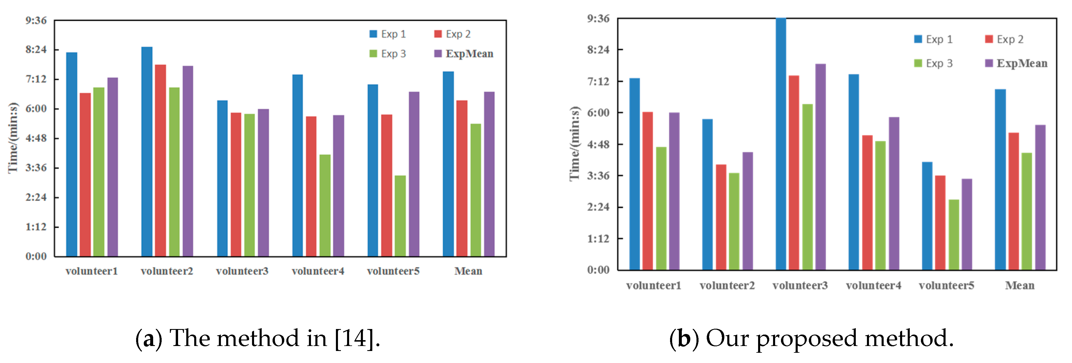
Evaluation index: This paper used the following two error index to measure the quality of the calibration in a simulation scenario. (1) SumIOD: The sum of the IOD [14] values of all internal parameters. (2) AbsRmsErr: The absolute root mean square re-projection error. The real internal parameters were known in the simulation scene, so the coordinate deviation of the same 3D coordinate points after the remapping of the real internal parameters could be calculated.
Experimental configuration: The properties of the simulated camera were set as follows: α = 1068 , β = 1073 , u 0 = 635 , v 0 = 355 , k 1 = 0.0031 , k 2 = 0.2059 , k 3 = 0.0028 , p 1 = 0.0038 , p 2 = 0.2478 . The parameters of pose search algorithm were set as follows: T 0 = 1 , T min = 0.1 , D = 0.7 , k = 10 . Gaussian noise with a mean value of 0 and a variance of 0.1 was introduced to simulate the error of feature point detection in a real scene [10]. Each group of experiments was repeated 20 times to take the average of the error. In the following four sets of experiments, the abscissa represents the number of frames, and the ordinate represents one of the error index. We used the log function based on e to process the results to make the comparison more obvious.
Performance evaluation of the proposed pose search algorithm: This experiment verifies the effectiveness of the proposed pose search algorithm. The initial solution of the algorithm was random pose and the loss function was AbsRmsErr. The comparison method used random pose for calibration. SumIOD and AbsRmsErr were used to evaluate the calibration result. The comparison results are shown in Figure 7. It can be seen that the pose obtained by searching had better performance for calibration.
Performance comparison of two loss functions: This experiment investigated the effect of loss function on the pose search algorithm. Based on using random pose as the initial solution, one method used AbsRmsErr as the loss function, and the other used SumIOD as the loss function. The comparison results are shown in Figure 8. It can be seen that SumIOD was superior to AbsRmsErr as a loss function.
Performance comparison of two initial solution methods: This experiment verified the effect of the initial pose method on the search algorithm. On the basis of using AbsRmsErr as the loss function, one method used the random pose as the initial solution, and the other used the generated pose as the initial solution. The comparison results are shown in Figure 9. It can be seen that the initial solution obtained from the generated pose method was better for searching for the optimal pose.
Performance comparison of different iterative calibration methods: This experiment compared the interactive calibration method in [14] with the pose search method proposed in this paper. Our search algorithm used the generating pose method to obtain the initial solution, and SumIOD was used as the loss function. The comparison results are shown in Figure 10. It can be seen that the pose search algorithm proposed in this paper could obtain a better pose for calibration.
Evaluation of the impact of frame number on running time. This experiment examined the magnitude of the change in the running time of our proposed method as the number of frames increases. The experiment was repeated 20 times and the average value was taken. The results are shown in Figure 11. It can be seen that the running time increased linearly with the increase of the number of frames. This is because the camera calibration time increased linearly as the number of pictures increased.

4.2. Real Data

Calibration performance evaluation comparison: In order to evaluate the proposed method on the measured data, 100 calibrated images with different positions and angles were captured in advance as the test set. All images were captured by the Dahua network camera with a resolution of 1280×720px. The proposed method was compared with the method in [14], OpenCV [32,33] without any pose constraints. The comparison results are shown in Table 1. Each method was calibrated five times and the average error was taken. The results showed that, compared with the method in [14], the proposed method had a 5.7% lower error when the number of calibration images was smaller. Compared with OpenCV, the error was reduced by 35.4%.
To evaluate the performance of the proposed pose decomposition method, we compared it with the method in [14] from two experiments: (1) the processing performance on continuous 5000 images; (2) the spend time to complete 10 poses in real scenarios for beginners.
Time comparison of image processing: The real-time calibration board detection brought an additional time delay for each image, which affected the efficiency of board placement. Table 2 gives the processing time on 5000 images based on different methods. The proposed camera calibration method consisted of the pose decomposition, projection, and preservation, while the method in [14] included the calibration board detection, three-dimensional coordinate system visualization, and target pose projection. It can be observed from Table 2 that the overall processing time was 19.23 s and 12.62 s respectively. The average processing time for each frame of the image was 38.46 ms and 25.24 ms respectively. The camera’s frame rate was 25 frames/s, that is, the delay per second was 0.961 s and 0.631 s respectively. The proposed method reduced the average processing time by 34.4% and it could address the time delay issue in the video stream.
Time consumption comparison of user guidance methods: To evaluate the proposed user guidance method (Pose decomposition) in this paper, we invited five volunteers to perform the calibration board placement task to match 10 preset poses. The time consumption of a user guidance method in [14] and our proposed method was compared. The time for each volunteer to complete these 10 pose matchings was recorded. Each volunteer used two methods repeated the experiment three times. The time consumption of the method in [14] is shown in Figure 12a and that of our proposed method is shown in Figure 12b. As can be seen from Figure 12, with the gradual familiarity of the user guidance method, the time required to complete 10 pose matching was gradually reduced. This reduction is particularly evident in Figure 12b. Based on pose decomposition and step-by-step guidance, the proposed method had a lower average time-consuming. The average time consumption was reduced by 17% compared with the method in [14].

5. Conclusions

In this paper, an interactive calibration system based on pose search and pose decomposition was proposed to estimate the camera internal parameters. The pose search method was designed to select the optimal pose for the calibration task in the entire pose space. A novel step-by-step user guidance method based on pose decomposition was proposed to improve the calibration efficiency. The proposed method was evaluated on both simulated and field datasets. Compared with the other interactive methods, the experimental results demonstrated our method can improve calibration effectiveness and efficiency.
Future work can be focused on the exploration of a novel evaluation index to improve search stability. In addition, the current interactive camera calibration methods only use a single camera, the binocular or multi-camera applications are required to achieve this task in the future.

Author Contributions

Conceptualization, W.L. (Wentai Lei) and M.X.; methodology, W.L. (Wentai Lei) and F.H.; software, M.X.; validation, T.X. and W.L. (Wenjun Li); formal analysis, W.J.; investigation, Y.L. and W.L. (Wenjun Li); resources, Y.Z. (Ye Zhao); data curation, W.J. and T.X.; writing—original draft preparation, M.X.; writing—review and editing, W.L. (Wentai Lei), C.W. and F.H.; visualization, C.W.; supervision, Y.L. and F.H.; project administration, W.L. (Wentai Lei) and Y.Z. (Yumei Zhao); funding acquisition, Y.Z. (Ye Zhao) and Y.Z. (Yumei Zhao) All authors have read and agreed to the published version of the manuscript.

Funding

This research was funded by the National Key R&D Program Safety Guarantee Technology of Urban Rail System, grant number 2016YFB1200402.

Conflicts of Interest

The authors declare no conflict of interest. The funders had no role in the design of the study; in the collection, analyses, or interpretation of data; in the writing of the manuscript, or in the decision to publish the results.

References

  1. di Lanzo, J.A.; Valentine, A.; Sohel, F.; Yapp, A.Y.T.; Muparadzi, K.C.; Abdelmalek, M. A review of the uses of virtual reality in engineering education. Comput. Appl. Eng. Educ. 2020, 28, 748–763. [Google Scholar] [CrossRef]
  2. Häne, C.; Heng, L.; Lee, G.H.; Fraundorfer, F.; Furgale, P.; Sattler, T.; Pollefeys, M. 3D Visual Perception for Self-Driving Cars using a Multi-Camera System: Calibration, Mapping, Localization, and Obstacle Detection. Image Vis. Comput. 2017, 68, 14–27. [Google Scholar] [CrossRef] [Green Version]
  3. Cai, Q. Research on Image-based 3D Reconstruction Technology. Master’s Thesis, Zhejiang University, Hangzhou, China, 2004. [Google Scholar]
  4. Guerchouche, R.; Coldefy, F. Camera calibration methods evaluation procedure for images rectification and 3D reconstruction. In Proceedings of the International Conference in Central Europe on Computer Graphics, Visualization and Computer Vision, Plzen, Czech Republic, 4–7 February 2008. [Google Scholar]
  5. Faig, W. Calibration of close-range photogrammetry systems: Mathematical formulation. Photogramm. Eng. Remote Sens. 1975, 41, 1479–1486. [Google Scholar]
  6. Qi, W.; Li, F.; Zhenzhong, L. Review on camera calibration. In Proceedings of the Chinese Control and Decision Conference, Xuzhou, China, 26–28 May 2010. [Google Scholar]
  7. Weng, J.; Cohen, P. Camera calibration with distortion models and accuracy evaluation. IEEE Trans. Pattern Anal. Mach. Intell. 1992, 14, 965–980. [Google Scholar] [CrossRef] [Green Version]
  8. Long, L.; Dongri, S. Review of Camera Calibration Algorithms. In Advances in Computer and Computational Sciences; Springer: Singapore, 2019; pp. 723–732. [Google Scholar]
  9. Zhan-Yi, H.U. A Review on Some Active Vision Based Camera Calibration Techniques. Chin. J. Comput. 2002, 25, 1149–1156. [Google Scholar]
  10. Zhang, Z. A Flexible New Technique for Camera Calibration. IEEE Trans. Pattern Anal. Mach. Intell. 2000, 22, 1330–1334. [Google Scholar] [CrossRef] [Green Version]
  11. Xie, Z.; Lu, W.; Wang, X.; Liu, J. Analysis of pose selection for binocular stereo calibration. Chin. J. Lasers 2015, 42, 237–244. [Google Scholar]
  12. Triggs, B. Autocalibration from Planar Scenes. In Proceedings of the European Conference on Computer Vision, Graz, Austria, 7–13 May 2006. [Google Scholar]
  13. Sturm, P.F.; Maybank, S.J. On plane-based camera calibration: A general algorithm, singularities, applications. In Proceedings of the IEEE Computer Society Conference on Computer Vision and Pattern Recognition, Fort Collins, CO, USA, 23–25 June 1999. [Google Scholar]
  14. Rojtberg, P.; Kuijper, A. Efficient Pose Selection for Interactive Camera Calibration. In Proceedings of the IEEE International Symposium on Mixed and Augmented Reality, Nantes, France, 9–13 October 2017. [Google Scholar]
  15. Richardson, A.; Strom, J.; Olson, E. AprilCal: Assisted and repeatable camera calibration. In Proceedings of the IEEE/RSJ International Conference on Intelligent Robots and Systems, Tokyo, Japan, 3–7 November 2013. [Google Scholar]
  16. Lazyloading. Available online: https://en.wikipedia.org/wiki/Lazy_loading (accessed on 5 November 2019).
  17. Fazakas, T.; Fekete, R.T. 3D reconstruction system for autonomous robot navigation. In Proceedings of the Computational Intelligence and Informatics, Budapest, Hungary, 18–20 November 2010. [Google Scholar]
  18. PinholeCamera. Available online: https://staff.fnwi.uva.nl/r.vandenboomgaard/IPCV20162017/LectureNotes/CV/PinholeCamera/index.html (accessed on 21 March 2020).
  19. Sun, W.; Cooperstock, J. Requirements for Camera Calibration: Must Accuracy Come with a High Price? In Proceedings of the IEEE Workshops on Applications of Computer Vision, Breckenridge, CO, USA, 5–7 January 2005. [Google Scholar]
  20. Heikkila, J.; Silven, O. A four-step camera calibration procedure with implicit image correction. In Proceedings of the IEEE Computer Society Conference on Computer Vision and Pattern Recognition, San Juan, PR, USA, 17–19 June 1997. [Google Scholar]
  21. Liu, Y.; Su, X. Camera calibration with planar crossed fringe patterns. Opt. Int. J. Light Electron Opt. 2012, 123, 171–175. [Google Scholar] [CrossRef]
  22. Yang, C.; Sun, F.; hu, Z. Planar conic based camera calibration. In Proceedings of the International Conference on Pattern Recognition, Barcelona, Spain, 3–7 September 2000. [Google Scholar]
  23. Moré, J. The Levenberg-Marquardt algorithm: Implementation and theory. Numer. Anal. 1978, 630, 105–116. [Google Scholar]
  24. Li, Z.; Ning, H.; Cao, L.; Zhang, T.; Gong, Y.; Huang, T.S. Learning to Search Efficiently in High Dimensions. In Advances in Neural Information Processing Systems; The MIT Press: Cambridge, MA, USA, 2012; pp. 1710–1718. [Google Scholar]
  25. SearchProblem. Available online: https://en.wikipedia.org/wiki/Search_problem (accessed on 15 January 2020).
  26. Simulated Annealing. Available online: https://en.wikipedia.org/wiki/Simulated_annealing (accessed on 10 February 2020).
  27. Konishi, T.; Kojima, H.; Nakagawa, H.; Tsuchiya, T. Using simulated annealing for locating array construction. Inf. Softw. Technol. 2020, 126, 106346. [Google Scholar] [CrossRef]
  28. Birdal, T.; Dobryden, I.; Ilic, S. X-Tag: A Fiducial Tag for Flexible and Accurate Bundle Adjustment. In Proceedings of the International Conference on 3D Vision, Stanford, CA, USA, 25–28 October 2016. [Google Scholar]
  29. Atcheson, B.; Heide, F.; Heidrich, W. CALTag: High Precision Fiducial Markers for Camera Calibration. In Proceedings of the Vision, Modeling, & Visualization Workshop, Siegen, Germany, 15–17 November 2010. [Google Scholar]
  30. Fiala, M.; Chang, S. Self-identifying patterns for plane-based camera calibration. Mach. Vis. Appl. 2008, 19, 209–216. [Google Scholar] [CrossRef]
  31. Garrido-Jurado, S. Detection of ChArUco Corners. Available online: http://docs.opencv.org/3.2.0/df/d4a/tutorial_charuco_detection.html (accessed on 7 February 2020).
  32. OpenCV Interactive Camera Calibration Application. Available online: https://docs.opencv.org/master/d7/d21/tutorial_interactive_calibration.html (accessed on 7 February 2020).
  33. Bradski, G. Learning-Based Computer Vision with Intel’s Open Source Computer Vision Library. Intel Technol. J. 2005, 9, 119. [Google Scholar]
Figure 1. The transformation diagram of a coordinate system.
Electronics 09 02170 g001
Figure 2. Schematic diagram of pinhole imaging model.
Electronics 09 02170 g002
Figure 3. The flow chart of our proposed calibration method.
Electronics 09 02170 g003
Figure 4. Five poses generated by C K group. The numbers in the figure indicate the order of pose generation.
Electronics 09 02170 g004
Figure 5. (a) Example of pose projection. (b) Example of pose decomposition projection. First, translate to the right of the image, and then rotate 30 degrees around the negative half axis of X-axis, and then rotate 39 degrees around the positive half axis of Y-axis, finally, rotate 22 degrees around the positive half axis of Z-axis.
Electronics 09 02170 g005
Figure 6. Positive rotation direction of the coordinate axis.
Electronics 09 02170 g006
Figure 7. No search (Random pose) vs. absolute root mean square re-projection error (AbsRmsErr) search (Random pose + AbsRmsErr loss). The green dotted line is obtained by the calibration method with the random pose. The magenta dotted line is obtained by our proposed pose search algorithm. The search algorithm takes a random pose as the initial solution and AbsRmsErr as the loss function.
Electronics 09 02170 g007
Figure 8. AbsRmsErr loss vs. sum of the index of dispersion (SumIOD) loss. The green dotted line is obtained by the pose search algorithm with AbsRmsErr as the loss function. The magenta dotted line is obtained by the pose search algorithm with SumIOD as the loss function. Both methods use a random pose as the initial solution.
Electronics 09 02170 g008
Figure 9. Random pose vs. Generated pose. The green dotted line is generated by the pose search algorithm with Random pose as the initial solution. The magenta dotted line is obtained by the pose search algorithm with a generated pose as the initial solution. Both methods use AbsRmsErr as the loss function.
Electronics 09 02170 g009
Figure 10. The method in [14] (Generated pose) vs. pose search (Generated pose + SumIOD). The green dotted line is generated by the method in [14]. The magenta dotted line is obtained by our proposed pose search algorithm, which takes a generated pose as the initial solution and SumIOD as the loss function.
Electronics 09 02170 g010
Figure 11. The curve of running time via the variance of frame number.
Electronics 09 02170 g011
Figure 12. Time consumption comparison between (a) the user guidance method in [14] and (b) the proposed method. The purple column represents the average value of three repeated experiments. The last group ‘Mean’ in both figures shows the average value of all volunteers.
Electronics 09 02170 g012
Table 1. Performance comparison of different methods.
Method Mean   φ t e s t Num. of Frames Mean   φ t r a i n
The method in [14]0.43318.80.5139
OpenCV0.6225390.43771
Our proposed method0.40867.80.4704
Table 2. Time comparison of different methods on image processing.
Method5000 Frames (s)Single Frame (ms)Delay Per Second (s)
The method in [14]19.2338.460.961
Our proposed method12.6225.240.631
Publisher’s Note: MDPI stays neutral with regard to jurisdictional claims in published maps and institutional affiliations.

