Estimating Micro-Level On-Road Vehicle Emissions Using the K-Means Clustering Method with GPS Big Data

Abstract

Due to the advanced spatial data collection technologies, the locations of vehicles on roads are now being collected nationwide, so there is a demand for applying a micro-level emission calculation methods to estimate regional and national emissions. However, it is difficult to apply this method due to the low data collection rate and the complicated calculation procedure. To solve these problems, this study proposes a vehicle trajectory extraction method for estimating micro-level vehicle emissions using massive GPS data. We extracted vehicle trajectories from the GPS data to estimate the emission factors for each link at a specific time period. Vehicle trajectory data was divided into several groups through a k-means clustering method, in which the ratios of each operating mode were used as variables for clustering similar vehicle trajectories. The results showed that the proposed method has an acceptable accuracy in estimating emissions. Furthermore, it was also confirmed that the estimated emission factors appropriately reflected the driving characteristics of links. If the proposed method were utilized to update the link-based micro-level emission factors using continuously accumulated trajectory data for the road network, it would be possible to efficiently calculate the regional- or national-level emissions only using traffic volume.

1. Introduction

Emissions from on-road mobile sources depend on the driving characteristics of the vehicles. The emission calculation methods are largely divided into macro-level approaches that consider the average speed of vehicles traveling along the roads as a driving characteristic and micro-level methods that reflect the change in instantaneous speed of individual vehicles as a driving characteristic [1]. Since the data on average speed, distance traveled (or link length), and traffic volume on the road section, which are necessary input data for calculating macroscopic emissions, is basically built and managed in the traffic network data, it is relatively easy to calculate the total emissions of the traffic network. For this reason, the macro-level emission estimation method has been generally applied and utilized for calculating the emissions from on-road mobile sources in different regions and countries [2,3,4]. However, in the macro-level emission estimation method using the average speed as the deterministic variable, the amount of vehicle emissions may be under- or overestimated because this method cannot capture the instantaneous changes in the vehicle driving speeds, such as stop-and-go traffic situations [5,6]. For this reason, there have been many claims that the micro-level emissions method should be applied in estimating regional and national emissions.

A number of previous studies have mounted GPS equipment onto only experimental vehicles to collect the vehicle trajectory data and estimate the vehicle emissions [7,8,9]. However, with the advancement of electronic communication technology, vehicle trajectories are being continuously collected nationwide by using vehicle navigation devices, digital tachographs (DTGs), and mobile devices, which have become available for estimating vehicle emissions [10,11,12]. The collection of vehicle trajectory data has become easier, and the range of spatio-temporal data collected has been expanded. As a result, it is possible to estimate micro-level emissions from the collected vehicle trajectory data.

However, there are some practical difficulties associated with adopting the micro-level approach at the regional and national levels. First, developing micro-level emission factors requires a large amount of time and cost. For vehicles with various fuel types, fleet sizes, and model years, it is necessary to conduct multiple driving tests, measure emissions under various operating conditions, and derive emission factors suitable for the micro-level emission estimation method. A fast solution is to use micro-level emission factor databases from other countries. In fact, the U.S. Environmental Protection Agency’s (U.S. EPA) Motor Vehicle Emission Simulator (MOVES) [13] can estimate micro-level vehicle emissions, and it has been applied in various studies from many countries [14,15,16,17,18] even though the approach should be taken with caution because the classification method for vehicle types and emission standards vary by country. The second problem is related to the acquisition of vehicle trajectory data, which is required to calculate micro-level vehicle emissions. In the case of collecting the link average speed of traffic flow, the average speed data can be easily collected from traffic information systems, such as loop detectors. However, estimating vehicle emissions with micro-level emission models is limited because it requires second-by-second vehicle trajectory data. It would be ideal to collect the trajectories of all vehicles driving along the roads to estimate the emissions of local or national on-road mobile sources on a micro-level basis, but that is highly impractical. Therefore, it would be useful to apply vehicle emissions, which are estimated at a micro level, at the regional and national levels with an easier and faster method.

This study proposes a representative vehicle trajectory extraction method for estimating micro-level vehicle emissions with a limited amount of vehicle trajectory data, such as that from DTGs or mobile devices. In the method, MOVES is used for analyzing vehicle emissions at a micro level, and vehicle trajectory data is divided into several groups through a k-means clustering method, in which the ratios of each operating mode (OpMode) in MOVES are used as cluster variables for clustering similar vehicle trajectories.

The rest of this paper is organized as follows: Section 2 describes the uniqueness of the representative vehicle trajectory extraction methodology used in this study, and Section 3 explains the proposed network-level micro-level emission estimation procedure, representative vehicle trajectory extraction method, and micro-level emission factor derived from this study. Section 4 presents the results of applying the proposed method to navigation data collected in Bucheon, Gyeonggi-do in Republic of Korea. Section 5 presents the effects of using the accumulated vehicle trajectory data on the method. In Section 6, the implications learned from the analysis results and the limitations of this study are discussed. The conclusions for this study are mentioned in Section 7.

2. Literature Review

To apply the micro-level emission estimation method to on-road mobile sources, it would be ideal to collect the trajectories of all vehicles running on the road and put the data into the micro-level emission calculation program. However, doing so is highly impractical, and even if it were not, it would be inefficient because it takes a large amount of time to calculate the micro-level emissions from all driving vehicles in the transportation network. To overcome this limitation, the U.S. EPA has developed MOVES [13], and several studies have incorporated vehicle trajectories (called driving cycles) into MOVES, which represent driving characteristics by vehicle type, road type, and level of service (LOS) [19,20,21,22]. However, it is not suitable to use the MOVES driving cycle in countries other than the United States because the road geometry, vehicle type composition ratio, and driver’s driving characteristics that determine the driving characteristics of a vehicle vary among countries [23,24]. Therefore, some studies conducted in countries other than the United States have applied MOVES with adjusted base emission rates to analyze vehicle emissions in those countries [19,20,21].

Another solution is to collect vehicle trajectory data from on-road mobile sources in the target area to be analyzed. The individual vehicle trajectories used in most studies were collected from a GPS device installed in a driving vehicle [7,8,9] or extracted from a microscopic traffic simulation model [25,26]. The vehicle trajectory data is collected or extracted from several vehicle types, including cars, trucks, and buses. Therefore, distinguishing the data by vehicle type is crucial for calculating vehicle emissions. Several studies have applied cluster analysis methods [27,28] to extract representative vehicle trajectories. Moreover, variables used to distinguish similar types of vehicle trajectories have included average speed, average acceleration, average deceleration, time proportion of idling mode/cruising mode/acceleration mode/deceleration mode/creeping mode, frequency of vehicle stops, mean length of driving period, average number of acceleration–deceleration changes, and root mean squared acceleration, which are aggregates representing the corresponding characteristics [29].

Previous studies associated with cluster analysis were performed to classify the vehicle trajectories into the representative driving cycles by vehicle type and road type. This study utilizes cluster analysis to assemble the vehicle trajectories of the same vehicle type on the same road section at the same time intervals into several similar vehicle trajectory groups and then uses the representative patterns of each group for estimating the corresponding highway link-based vehicle emissions. This process is expected to reflect the various driving situations that can occur in the same context. If aggregated characteristics, such as average speed and maximum acceleration, are used as variables for clustering, these measures cannot be used for micro-level emission estimation. Thus, the MOVES OpMode distribution, which can be used immediately for estimating micro-level vehicle emissions in MOVES, is applied as a variable for cluster analysis.

3. Methods

3.1. Micro-Level Emission Estimation Method Using Individual Vehicle Trajectory Data

3.1.1. Micro-Level Emission Factor

The MOVES’s micro-level emission estimation methodology is applied to calculating emissions with trajectories of individual vehicles collected from vehicle navigation, odometer (i.e., DTG), and mobile devices. The MOVES database stores the basic emission factors for each pollutant at OpMode by each vehicle type, which is subdivided by fuel use, size, year of manufacture, and vehicle age. MOVES provides the result of calculating the emissions according to various conditions, such as the vehicle type composition ratio, fuel compound characteristics, and temperature and humidity on the road section.

In this study, the base emission rates for each vehicle type from the MOVES database are applied to calculate the basic emission factors at the OpModes of passenger cars, trucks, and buses, as shown in Appendix A, Appendix B, and Appendix C. In order to make these tables, the ratios of each subdivided vehicle type (size, fuel, vehicle age) of the target year 2017 in Bucheon, Gyeonggi-do, which is an analysis target area collected from the Korea vehicle registration information, are used as weighted values. CO, NO_x, PM₁₀, PM_2.5, and CO₂ are selected as the pollutants to be estimated, and the unit of the emission factors is g/sec. The emissions are calculated in this study without considering the adjustment for climatic conditions.

3.1.2. MOVES OpMode

Location information in the vehicle trajectory of an individual vehicle was collected from vehicle navigation and DTG data. After the speed per second is calculated with the distance from the change in vehicle location per second, the acceleration per second can be calculated. Then, the vehicle-specific power (VSP) per second is calculated with Equation (1), which is an equation for MOVES VSP [30]. The terms A, B, and C have different values for each vehicle type, and a suitable value for the corresponding vehicle type among the values presented in MOVES should be found and applied. Next, OpMode per second is found among 23 OpModes according to the VSP range and speed range (see Appendix A, Appendix B, Appendix C):

$$P_{V,t} = \frac{A{v}_t + B{v}_t^2 + C{v}_t^3 + m{v}_t\left(a_t + gsin{\theta }_t\right)}{m}$$

(1)

where $P_{V,t}$: VSP (kW/ton) for vehicle V at time t, t: time (s), $v_t$: speed ($\mathrm{m}/{\mathrm{s}}^2$), $a_t$: acceleration ($\mathrm{m}/{\mathrm{s}}^2$), m: weight (ton), A: rolling resistance ($\mathrm{KWsec}/\mathrm{m}$), B: rotating term (${\mathrm{KWsec}}^2/{\mathrm{m}}^2$), C: aerodynamic drag term (${\mathrm{KWsec}}^3/{\mathrm{m}}^3$), g: acceleration due to gravity (9.81 $\mathrm{m}/{\mathrm{s}}^2$) and ${\theta }_t$: road grade (degrees).

After finding the emissions per second corresponding to the OpModes from the emission factor table of the corresponding vehicle type, the emissions from the vehicle are calculated through the aggregation process. When it is necessary to aggregate the emissions by road section on the traffic network, the location information per second can be utilized to match the link ID suitable for the node ID and link ID of the traffic network, and the emissions for each link can be calculated.

3.2. Extraction of Representative OpMode Distribution and Estimation of Micro-Level Emission Factors

3.2.1. Concept

Emissions from individual vehicles can be estimated with vehicle trajectory data collected from GPS devices by the method described in Section 3.1. The problem is that the total amount of emissions cannot be calculated because it is not possible to collect the driving trajectory data from all vehicles in the target area. One way to consider is to make the extracted vehicle trajectories from the results of the microscopic traffic simulation network model, which can replace the actual vehicle trajectories. However, it has several disadvantages. First, it is not easy to calibrate a traffic simulation network model to make it similar to the actual traffic network. Second, if the target area is changed, the method can be applied only after establishing a new simulation network for that area. Furthermore, even if this method enables all the vehicle trajectories of the entire network to be acquired, calculating emissions from all vehicles in a large network using the micro-level emission estimation method would require a lot of time.

Another alternative is to find representative vehicle trajectories on the target road section at the analysis time interval for each vehicle type (passenger cars, trucks, buses), calculate emissions from those vehicles’ trajectory data, and use the calculation results to estimate emissions from all vehicles in the road section at the analysis time interval. Because the traffic volume for each vehicle type in the analysis time interval of the target road can be obtained by using ITS equipment or the traffic volume estimation model, the total emissions can be calculated by multiplying the traffic volume by the emissions from the representative vehicle trajectories. This method has the advantage of higher efficiency in calculating regional vehicle emissions because the calculated emissions based on the representative vehicle trajectories from each road section can be used as emission factors (g/veh) for each road section. On that basis, in this study, this method has been applied to extract the trajectory of a vehicle, which has representative driving characteristics, from the vehicle trajectory data of some vehicles that passed the corresponding road section at the corresponding time interval.

Several studies aimed at developing representative vehicle trajectories have been established. For example, a representative link driving cycle by vehicle type, road type, and LOS has been developed for MOVES. However, it is not appropriate to apply their driving cycles to estimate regional vehicle emissions. The first reason is that the concept of the measurement link of the MOVES driving cycle is different from the link in the transportation network of the node link system. The former is closer to the travel route concept, while the latter refers to a road section whose length can vary and is shorter than a travel route. The second reason is that the concept of driving cycle is different between the MOVES driving cycles and the extracted representative link vehicle trajectories in this study. The MOVES driving cycles are developed to represent vehicle driving characteristics of various road types. On the other hand, this study extracts the representative vehicle trajectories to reflect the various driving situations that can appear in each link based on the driving data collected from each link. In other words, the driving characteristics of the same vehicle type that runs on the same road at the same time interval should have many similarities, as well as certain differences. For example, in the case of an arterial road, there will be a difference in vehicle trajectories between a vehicle experiencing traffic delay due to signals and one that is not. Thus, this study intends to classify vehicle trajectories into several similar groups and use the center of each group as a representative vehicle trajectory.

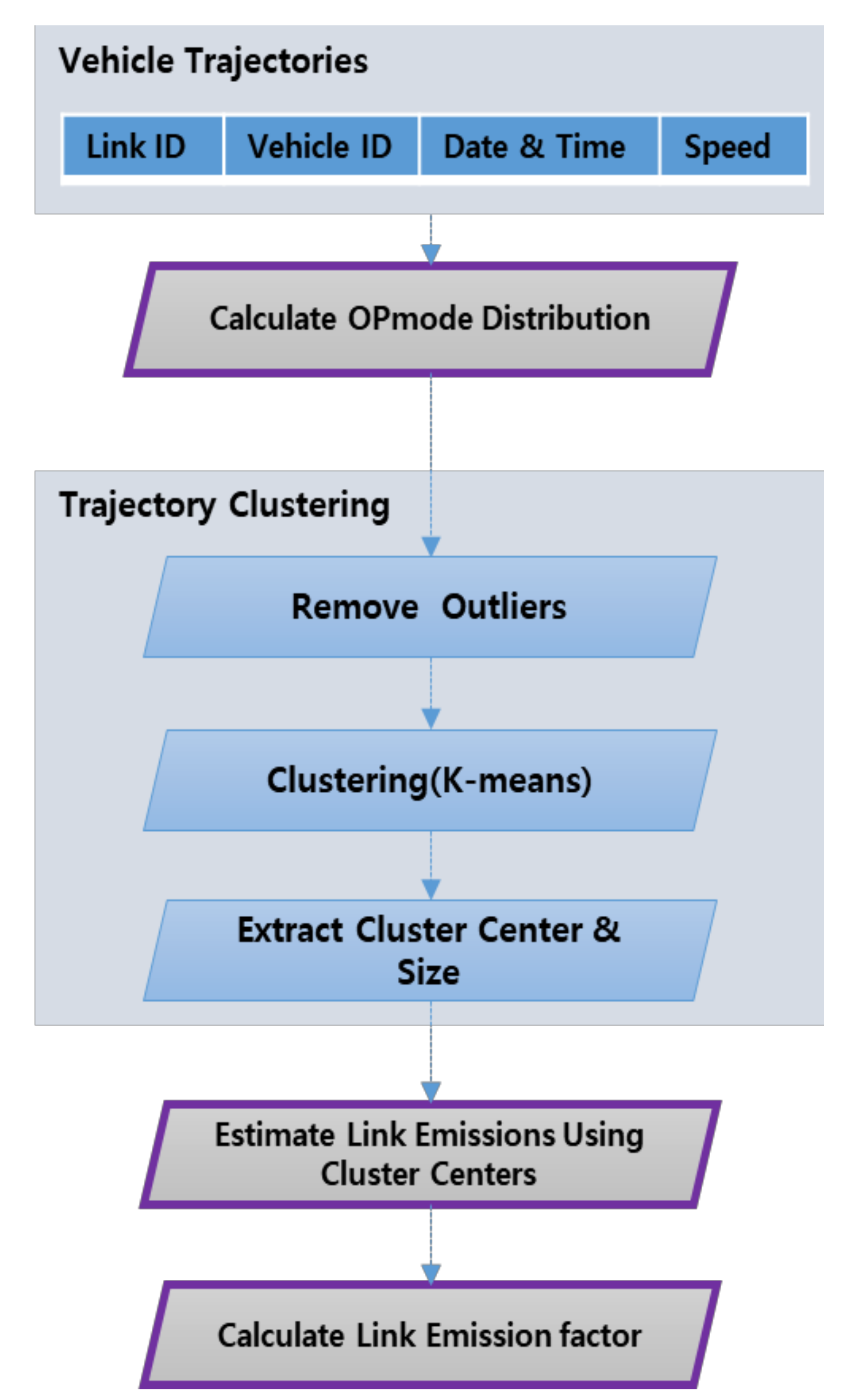
Figure 1 is a diagram showing the procedure for estimating the micro-level link emission factors required to calculate the emissions at the network level by using the collected vehicle trajectory data. The following section explains each process in detail.

3.2.2. Calculate OpMode Distribution of Vehicle Trajectory

First, the vehicle trajectories of the same vehicle type on the same road section at the same time interval are collected. The vehicle trajectory data includes link ID, vehicle ID, recording time, and speed at each time point (in sec). Second, the VSP per second is calculated by the method described in Section 3.1.2 for each vehicle trajectory, and OpModes per second are classified for each vehicle trajectory. Then, the frequency for each of the 23 OpModes is calculated, and the ratios of each OpMode are calculated and stored. Each vehicle trajectory has 23 new variables, which are the ratios of each OpMode.

3.2.3. Trajectory Clustering

Before performing cluster analysis, outliers are removed from the vehicle trajectory dataset to filter out unusual driving cases that have not passed through the entire link or have stopped for a long time. Cluster analysis is performed to assemble the data into several similar vehicle trajectory groups. The k-means method is used to find the optimal number clusters and the center of each cluster. As a variable for each cluster analysis, the ratio by OpMode, which can describe the characteristics of the vehicle trajectory, is used. As in previous studies, aggregated characteristics, such as average speed and maximum acceleration, could be used as variables for clustering, while the ratio for each OpMode was selected as a cluster analysis variable. The main purpose is to utilize the value of the center of each group, which is the OpMode distribution, for micro-level emission calculation. Another purpose is to use the same scaled cluster variables. Using the values of the cluster center, the emissions of the cluster center can be calculated. The weighted average of emissions of all vehicles is obtained by applying the cluster size as a weight, which means the emissions per vehicle on the corresponding road section. It can be used as a micro-level link emission factor.

3.2.4. Calculate Link Emission Factor

After cluster analysis, the OpMode distribution and cluster size of each cluster center are extracted, which are used to calculate the emissions of all clusters by Equation (2):

$${\mathrm{Emissions}}_{pol} = {{\displaystyle \sum }}_1^k\left({({{\displaystyle \sum }}_{}^{opmode}{R}_{opmode } * E{F}_{opmode, pol})}_k * siz{e}_k * meanTT\right),$$

(2)

where ${({{\displaystyle \sum }}_{}^{opmode}{R}_{opmode}*E{F}_{opmode,pol})}_k:$ represents the emissions of cluster k, $R_{opmode }$ is the ratio of each OpMode, $E{F}_{opmode, pol}$ the OpMode emission factors by pollutants (pol, in g/sec), $k$ is the cluster number, $siz{e}_k$ is the cluster size and $meanTT$ is the average driving time of vehicle trajectories

Finally, as shown in Equation (3), by dividing the total emissions by the total number of vehicles used in the cluster analysis, the micro-level link emission factor of the vehicle type is calculated by the following:

$$micLE{F}_{ pol} = {\mathrm{emissions}}_{pol}/\mathrm{number}\mathrm{of}\mathrm{vehicles}$$

(3)

where $micLE{F}_{pol}:$ micro-level emission factor (g/veh).

According to the collected vehicle trajectory data, the data will be spatio-temporally expanded and applied to the regional and national levels. A database of micro-level link emission factors for a nationwide traffic network can be established. The procedure for estimating the micro-level link emission factors should be performed by vehicle type and analysis time interval on each road section. When a vehicle type-specific traffic volume database is provided, the emissions from all the vehicles on the traffic network will be easily calculated by applying the database of micro-level link emission factors for a nationwide traffic network.

4. Case Study

In the case analysis, emissions were estimated based on the method described in Section 3 by using the navigation data collected from actual roads, and it was investigated whether such a method produces accurate emission calculation results as intended. As the target roads, as shown in Figure 2, one section of the highway (about 1 km long) and one section of the arterial road (about 600 m long) in Bucheon, Gyeonggi-do in the Republic of Korea are selected to inspect whether the method reflects the driving characteristics of uninterrupted flow and interrupted flow, respectively. The target road sections are shown in Figure 2, and their attributes are described below.

• Selected freeway link

  ∘

  Road name: Seoul Jeil Sunwhan Expressway

  ∘

  Number of lanes: Four per direction

  ∘

  Speed limit: 100 km/h

• Selected arterial link

  ∘

  Road name: Sosaro

  ∘

  Number of lanes: two per direction

  ∘

  Speed limit: 60 km/h

4.1. Data Collection

The navigation data was acquired in December 2017, and among the data on 13 December (Wednesday), the driving data on the morning peak hours (07:00–09:00), non-peak hours (13:00–15:00), and afternoon peak hours (17:00–19:00) for the northbound and southbound parts of each road section was extracted.

Table 1. Acquired vehicle trajectories.

			Total Number of Trajectories	Traffic Volume 4 (veh/hour)	Collecting Ratio
Freeway Link	North bound	AM peak1	288	7128.5	2.0%
		Off peak2	430	7284.5	3.0%
		PM peak3	382	7527	2.5%
	South bound	AM peak	364	4487	4.1%
		Off peak	608	4062	7.5%
		PM peak	508	4022.5	6.3%
Arterial Links	North bound	AM peak	51	1375.5	1.9%
		Off peak	83	1440.5	2.9%
		PM peak	98	1635.5	3.0%
	South bound	AM peak	50	1709	1.5%
		Off peak	81	1268.5	3.2%
		PM peak	98	1289	3.8%

¹ 07:00–09:00, ² 13:00–15:00, ³ 17:00–19:00, ⁴ Estimated traffic volume provided by the Korean Traffic Database.

summarizes the number of vehicle trajectories collected for each analysis unit, showing that the vehicle trajectories corresponding to approximately 2–7% of the traffic volume were collected. After extracting the vehicle position in seconds from the navigation data, the data was organized into vehicle-specific driving trajectory data to calculate the speed per second and acceleration per second. Because most of the navigation data was provided from passenger cars, the analysis was conducted by considering the passenger car as the vehicle type.

4.2. Cluster Analysis Results

Cluster analysis was performed for each of the 12 groups listed in Table 1, and

Table 2. Summary of trajectory clustering.

	Freeway
	Northbound			Southbound
Time Period	AMpeak	offpeak	PMpeak	AMpeak	offpeak	PMpeak
Total trajectories	288	430	382	364	608	508
ATT, Average travel time (s)	111.84	138.16	90.86	234.8	163.77	176.55
Outlier upper limit (s)	−82.5	−70.75	−80.5	−360.5	−88	−178
Outlier lower limit (s)	217.5	207.25	223.5	819.5	360	526
Selected trajectories	74	134	92	95	110	125
ATT (s) of selected trajectories	103.27	99.26	107.16	93.18	90.8	100.46
Best number of Clusters	7	7	8	8	7	8
Clustering Fitness	0.7944	0.7068	0.6906	0.7131	0.6563	0.6269
	Arterial
	Northbound			Southbound
Time period	AMpeak	offpeak	PMpeak	AMpeak	offpeak	PMpeak
Total trajectories	51	83	98	50	81	98
ATT, Average travel time (s)	279.1	286.19	318.23	280.9	271.28	306.7
Outlier upper limit (s)	−439.75	−45.88	−60.75	−449	−81	−67
Outlier lower limit (s)	998.75	388.38	621.25	983	378	597
Selected trajectories	22	23	21	19	20	21
ATT (s) of selected trajectories	515.05	193.7	240.29	525.21	185.8	243.43
Best number of Clusters	6	6	8	7	6	8
Clustering Fitness	0.9284	0.8407	0.8693	0.9502	0.8001	0.9033

summarizes the results. Among the collected vehicle trajectories, the data showing outliers in terms of the travel time was removed before the cluster analysis. Most of the removed vehicle trajectories were from vehicles that did not pass through all sections of the corresponding road. Table 2 shows the criteria for outlier removal and the number of selected vehicle trajectories. The cluster analysis results reveal that the best number of clusters for highway data is 7 to 8 and the ratio of goodness of fit is about 0.6 to 0.8. The results also show that the best number of clusters for the arterial road data is 6 to 8 and the ratio of goodness of fit is about 0.8 to 0.9.

4.3. Emission Estimation Results

The emissions of air pollutants (CO, NO_x, PM₁₀, PM_2.5, and CO₂) were estimated based on the method described in Section 3. The estimated emissions were compared with the results obtained by estimating emissions using each individual vehicle trajectory through the micro-level emission estimation method of MOVES. As shown in

Table 3. Comparison of link emission estimation results.

Freeway Northbound
	AMpeak			offpeak			PMpeak
	A 1	B 2	R 3	A	B	R	A	B	R
CO (g)	94.6	97.55	1.03	156.98	158.23	1.01	113.87	116.67	1.02
NOx (g)	4.46	4.624	1.04	8.128	8.248	1.01	5.868	6.091	1.04
PM2.5 (g)	0.0227	0.0236	1.04	0.0366	0.0369	1.01	0.0254	0.0261	1.03
PM10 (g)	0.0254	0.0265	1.04	0.0414	0.0417	1.01	0.0282	0.029	1.03
CO2 (g)	16,417.48	16,636.82	1.01	29,423.6	29,484.94	1.00	21,554.42	21,865.07	1.01
Freeway Southbound
	AMpeak			offpeak			PMpeak
	A	B	R	A	B	R	A	B	R
CO (g)	124.12	125.22	1.01	128.17	129.48	1.01	149.25	150.85	1.01
NOx (g)	5.994	6.047	1.01	6.943	7.05	1.02	7.957	8.107	1.02
PM2.5 (g)	0.0309	0.0313	1.01	0.0299	0.0302	1.01	0.0335	0.0339	1.01
PM10 (g)	0.0348	0.0352	1.01	0.0334	0.0337	1.01	0.0373	0.0378	1.01
CO2 (g)	20,139.64	20,127.88	1.00	23,156.19	23,252.67	1.00	28,295.29	28,363.63	1.00
Arterial Northbound
	AMpeak			offpeak			PMpeak
	A	B	R	A	B	R	A	B	R
CO (g)	53.48	56.78	1.06	27.45	28.52	1.04	29.06	30.12	1.04
NOx (g)	1.931	2.043	1.06	1.012	1.061	1.05	1.051	1.089	1.04
PM2.5 (g)	0.0153	0.0158	1.03	0.0067	0.0069	1.03	0.0075	0.0077	1.03
PM10 (g)	0.0223	0.0228	1.02	0.0089	0.0091	1.02	0.01	0.0102	1.02
CO2 (g)	13,893.62	14,425.56	1.04	6248.72	6437.99	1.03	6790.39	7006.47	1.03
Arterial Southbound
	AMpeak			offpeak			PMpeak
	A	B	R	A	B	R	A	B	R
CO (g)	47.46	48.7	1.03	24.04	24.32	1.01	29.91	30.25	1.01
NOx (g)	1.719	1.786	1.04	0.876	0.896	1.02	1.086	1.098	1.01
PM2.5 (g)	0.0137	0.0138	1.01	0.0058	0.0059	1.02	0.0077	0.0077	1.00
PM10 (g)	0.02	0.02	1.00	0.0076	0.0076	1.00	0.0104	0.0104	1.00
CO2 (g)	12,413	12,601.47	1.02	5398.06	5422.57	1.00	7041.24	7069.78	1.00

¹ Estimating emissions using each individual vehicle trajectory through the micro-level emission estimation method of MOVES, ² Estimating emissions using emissions of cluster centers through the proposed method, ³ B/A.

, the difference in the emissions calculated by the two methods is insignificant, at 1–4% for the highway and 1–6% for the arterial road. The results prove that the proposed method has acceptable accuracy in estimating emissions.

4.4. Micro-Level Link Emission Factors

The micro-level link emission factors are calculated by emissions from vehicles in all clusters, which are B columns in Table 3 by the number of vehicles (the number of vehicle trajectories), and summarized in

Table 4. Estimated link emission factors (g/veh).

	Freeway
	Northbound			Southbound
Time Period	AMpeak	offpeak	PMpeak	AMpeak	offpeak	PMpeak
CO	1.32	1.18	1.27	1.32	1.18	1.21
NOx	0.0625	0.0616	0.0662	0.0637	0.0641	0.0649
PM2.5	0.000319	0.000275	0.000284	0.000329	0.000275	0.000271
PM10	0.000358	0.000311	0.000315	0.000371	0.000306	0.000302
CO2	224.82	220.04	237.66	211.87	211.39	226.91
	Arterial
	Northbound			Southbound
Time Period	AMpeak	offpeak	PMpeak	AMpeak	offpeak	PMpeak
CO	2.58	1.24	1.43	2.56	1.22	1.44
NOx	0.0929	0.0461	0.0519	0.0940	0.0448	0.0523
PM2.5	0.000718	0.000300	0.000367	0.000726	0.000295	0.000367
PM10	0.001036	0.000396	0.000486	0.001053	0.000380	0.000495
CO2	655.71	279.91	333.64	663.24	271.13	336.66

. These values are the micro-level emission factors of the passenger car at the analysis time interval on the analysis link for each pollutant. As shown in Figure 3, plotting these values through bar graphs can determine whether the estimated micro-level link emission factors can appropriately reflect the emission characteristics of the link. The emission factors show the highest trend in the morning peak hours and the lowest in the non-peak hours, indicating the change in emissions according to time periods of the link. Even though the driving length of the highway (about 1 km) is longer than that of the arterial road (about 600 m), the emissions are lower on the highway, which indicates that the emission factors appropriately reflect the driving characteristics by the road characteristics (uninterrupted flow and interrupted flow) of the link.

5. Effects on Clustering and Micro-Level Link Emission Factors by Using Accumulated Vehicle Trajectories

This study has confirmed that the proposed method can be applied to estimate the total emissions from vehicles traveling on a road section with the actual vehicle trajectory data through the case study. Micro-level link emission factors for links were derived through the proposed emission estimation process using vehicle trajectories collected from one day. This method may be applied by using accumulated vehicle trajectory data collected over several days to increase the micro-level link emission factors’ representativeness. Use of an accumulated dataset can offset the limitations of vehicle trajectory data, which have a low rate of acquisition, and enable the analysis time period to be divided into shorter periods to increase detail.

To analyze the effect of using accumulated vehicle trajectory data, the vehicle trajectory data of the freeway northbound link selected for the case study was additionally acquired. The trajectory data of the vehicles traveling through the road section during the 2-h morning peak on weekdays (Tuesday, Wednesday, and Thursday) in December 2017 was used. A total of 12 datasets were made by increasing the number of data collection days from one day to 12 days. For example, the first dataset included one day of data, the second dataset included an additional day of data, and so on. The proposed method was applied to each of those datasets.

In this analysis, changing patterns in cluster analysis results and estimated micro-level emission factors were investigated by accumulating daily data.

Table 5. Vehicle trajectory selection results.

Days	12/5	12/6	12/7	12/12	12/13	12/14
Total trajectories	301	253	264	288	288	282
ATT, Average travel time (s)	102.41	104.87	125.31	134.15	111.84	106.4
Outlier upper limit (s)	−66.25	−92.12	−66.5	−71.5	−82.5	−59
Outlier lower limit (s)	196.25	247.12	217.5	220.5	217.5	205
Selected trajectories	80	67	81	93	74	91
ATT (s) of selected trajectories	92.85	112.73	103.69	100.72	103.27	98.21
Days	12/19	12/20	12/21	12/26	12/27	12/28
Total trajectories	283	303	246	261	300	314
ATT, Average travel time (s)	114.8	93.67	87.94	98.64	95.41	92.2
Outlier upper limit (s)	−59.88	−59.88	−74.5	−64	−71	−84.25
Outlier lower limit (s)	205.38	201.38	217.5	192	209	225.75
Selected trajectories	101	92	72	76	103	99
ATT (s) of selected trajectories	102.94	97.85	104.21	93.21	103.65	104.32

shows the number of remaining vehicle trajectories after removing outliers among the vehicle trajectories collected on each date.

Table 6. Summary of trajectory clustering by increasing number of data collection days.

Days	1 day	2 days	3 days	4 days	5 days	6 days
Selected trajectories	80	147	228	321	395	486
ATT (s) of selected trajectories	92.85	101.91	102.54	102.02	102.25	101.49
Best number of clusters	7	7	7	7	7	7
Clustering Fitness	0.7195	0.7723	0.7474	0.7563	0.754	0.7379
Days	7 days	8 days	9 days	10 days	11 days	12 days
Selected trajectories	587	679	751	827	930	1029
ATT (s) of selected trajectories	101.74	101.22	101.5	100.74	101.06	101.38
Best number of Clusters	7	7	7	7	7	7
Clustering Fitness	0.7345	0.7343	0.729	0.7244	0.7254	0.7228

summarizes the cluster analysis results subject to daily accumulation of the data, which shows that the number of vehicle trajectories used for cluster analysis increases as the daily data is accumulated, reaching 1029 after the 12th day of accumulation. The average travel times of the vehicle trajectories used for cluster analysis show a pattern that converges to about 101 s. The optimal number of clusters is 7, and the ratio of goodness of fit is 0.7 or more.

Figure 4 is a diagram comparing the OpMode distributions of seven cluster centers derived from each dataset. It can be observed that the shapes of the OpMode distribution of the seven cluster centers are similar after Day 4. This graph offers useful information for determining how many days are required to accumulate vehicle trajectories for estimating micro-level link emission factors.

Table 7. Estimated link emission factors (g/veh) by adding number of data collection days.

Days	1 day	2 days	3 days	4 days	5 days	6 days
CO	1.398625	1.360816	1.32943	1.321153	1.320658	1.326461
NOx	0.0661	0.064524	0.062522	0.062414	0.06243	0.062914
PM2.5	0.000356	0.000335	0.000325	0.000323	0.000322	0.000324
PM10	0.000403	0.000379	0.000368	0.000366	0.000364	0.000366
CO2	213.4434	224.6081	223.2107	222.4063	222.8595	222.4115
Days	7 days	8 days	9 days	10 days	11 days	12 days
CO	1.323799	1.326966	1.322703	1.33162	1.326516	1.317891
NOx	0.062833	0.062929	0.062848	0.063204	0.063115	0.062888
PM2.5	0.000323	0.000324	0.000323	0.000326	0.000324	0.000321
PM10	0.000365	0.000367	0.000365	0.000368	0.000366	0.000363
CO2	222.6467	222.0059	222.3667	221.6501	222.0375	222.2886

summarizes the micro-level emission factors for each pollutant estimated by adding the number of data collection days. The bar graphs plotted in Figure 5 show that the micro-level emission factors tend to converge as the number of days of data accumulation increases. It means that the estimated micro-level link emission factors’ representativeness increases as the data is accumulated.

6. Discussion

The applicability of the developed methodology was examined by using the navigation data collected according to each of the three (morning peak hours, non-peak hours, afternoon peak hours) analysis time intervals on one highway section (1 km) and one arterial road section (600 m). The results of the analysis confirmed that the error rate showed a difference in the range of 1–4% for the highway section and 1–6% for the arterial road section when the link emissions were calculated using the proposed method. Moreover, the results indicated that the estimated micro-level link emission factors reflect the driving characteristics of the link according to the traffic conditions for each time period and the driving characteristics for each road characteristic (uninterrupted flow and interrupted flow). Additionally, the analysis results through the same method while accumulating the vehicle trajectory data showed that clustering analysis produced similar cluster centers after 4-day data accumulation and link emission factors were converged to certain values representing the vehicle travel characteristics on the corresponding road at the corresponding time period by adding the number of data collection days. The number of days to reach convergence on the target road in this study was about four, while it is expected to increase in road sections having fewer collected vehicle trajectories. These results mean that the proposed method can offset the limitations of vehicle trajectory data with a small number of samples. Furthermore, this approach enables the analysis time period to be shorter and thus the micro-level emission calculation of the entire network to be analyzed in more detail.

In this study, because navigation data was used, the results were limited to the case of passenger cars. Therefore, it is necessary to acquire the vehicle trajectories of a commercial vehicle, such as a truck or bus, from DTG data to check whether the applicability is the same. In addition, considering that the link length of the traffic network varies, it is also necessary to vary the collected link length to check whether there are any points to be supplemented in the analysis method. Moreover, it is also required to confirm the basis for judgment as to how many days for data accumulation and analysis would enable representative link micro-level emission factors to be developed.

7. Conclusions

Several problems must be addressed to apply the micro-level emission estimation method at the regional or national level by using the vehicle trajectory data collected through GPS data. The biggest problem is that it is not possible to collect the vehicle trajectory data of all vehicles running on the traffic network. The second problem is related to the task of extracting necessary data from the collected vehicle trajectory, which requires a considerable amount of data processing and operation time in calculating the micro-level emissions of individual vehicles and aggregating results by road section.

This study proposed a countermeasure to solve these problems. In this study, a micro-level emission estimation method using the massive vehicle trajectory data collected from vehicle navigation, DTG, and mobile devices was developed, which can be applicable at the regional or national level. The vehicle trajectories from collected GPS data were classified as link ID and time period to estimate the emissions and emission factors for each link at a specific time period. Vehicle trajectories for a link at a time period were divided into several groups through cluster analysis, in which the ratios of each OpMode used in MOVES were used as cluster variables for clustering similar vehicle trajectories. The choice of cluster variables is the biggest difference from the other methods for clustering vehicle trajectories. The derived values of each cluster center from clustering analysis, the OpMode distribution, can be used for calculating micro-level emissions. The center of each cluster denotes the representative vehicle trajectory for each cluster. The emissions of the cluster center can be calculated easily by using the values of the cluster center. The weighted averages of emissions of all vehicles are obtained by applying the cluster size as a weight, which represents the emissions per vehicle on the corresponding road section. They can be used as micro-level link emission factors to estimate emissions of regional- or national-level traffic networks. When vehicle type-specific traffic volume is provided, the emissions from all the vehicles on the traffic network will be easily calculated by multiplying by the micro-level link emission factors. This is the main purpose of developing the proposed method.

The proposed method is not free from computational difficulty because the operating distribution of each vehicle trajectory must be calculated to estimate link-based micro-level emission factors. Moreover, more data must be collected and analyzed in order to increase the representativeness. This requires more storage space and computing power. Fortunately, not only can the calculation procedures of the proposed method be automated but also high-performance machines can be utilized for the calculation. Thus, it is expected that the issues of storage space and computing power related to the proposed method can be addressed.

The confirmation procedure explained in the previous section is still required. However, if the proposed method were automated to accumulate data, such as navigation data, DTG data, and mobile data, for each traffic network link and update the link-based micro-level emission factors, only having traffic volume by vehicle type at the analysis time period would enable local or nationwide micro-level emission estimation to be performed efficiently.