A Review on Deep Learning-Based Approaches for Automatic Sonar Target Recognition

Abstract

Underwater acoustics has been implemented mostly in the field of sound navigation and ranging (SONAR) procedures for submarine communication, the examination of maritime assets and environment surveying, target and object recognition, and measurement and study of acoustic sources in the underwater atmosphere. With the rapid development in science and technology, the advancement in sonar systems has increased, resulting in a decrement in underwater casualties. The sonar signal processing and automatic target recognition using sonar signals or imagery is itself a challenging process. Meanwhile, highly advanced data-driven machine-learning and deep learning-based methods are being implemented for acquiring several types of information from underwater sound data. This paper reviews the recent sonar automatic target recognition, tracking, or detection works using deep learning algorithms. A thorough study of the available works is done, and the operating procedure, results, and other necessary details regarding the data acquisition process, the dataset used, and the information regarding hyper-parameters is presented in this article. This paper will be of great assistance for upcoming scholars to start their work on sonar automatic target recognition.

1. Introduction

Underwater acoustics, the mutual domain for the analysis of all the processes associated with the generation, occurrence, transmission, and reception of sound pulses in the water medium and its interference with boundaries, has mostly been implemented to submarine communication, the examination of maritime assets and environment surveying, target and object recognition, and measurement and study of acoustic sources in underwater atmosphere. Remote sensing, which can be described as a sonar system, is applied when a target of interest cannot be directly verified, and the information about it is to be gained secondarily [1]. Sonar, a collective term for numerous devices that use sound waves as the information carrier, is a technique that permits ships and other vessels to discover and recognize substances in the water through a system of sound rhythms and echoes [2]. It can accomplish detection, location, identification, and tracking of targets in the marine environment and perform underwater communication, navigation, measurement, and other functions [3]. In the past few years, the use of sonar equipment is bursting forth. Because of the extreme fading of radio frequencies and visual signals in the water medium, acoustic waves are mostly considered powerful methods to sense underwater objects and targets [4]. The sound waves can travel farther in water than the radio waves or radar [5]. The earliest sonar-like device was invented in 1906 by naval architect Lewis Nixon. It was designed to help ships in navigating properly by sensing icebergs under the water [2]. An inflection point for the sonar system and the furtherance of its derivations is the 1912 Titanic catastrophe, which turned out the sonar system as one of the highly developed engineering systems [6].

The fundamental theory of a sonar system contains the propagation of sound energy into the water medium and the reflected waves’ reception from objects or seafloor. The sonar produces short electric waves, which are in sound waves form at a specific length, frequency, and energy, with the help of a transmitter. The transducer transforms these electrical signals into mechanical vibration energy; these vibrations afterward are transferred into the water as the pulse, traveling through the water medium until the reflection occurs. The transducer again converts those reflected energies in the mechanical form into electrical energy. This electrical energy is sensed and amplified by the sonar receiver. A master unit has a control function for synchronizing the actions and control timing for the broadcasting and reception of the electric signal. The control unit usually has a unit to show the received data [7]. Analyzing the incoming underwater sound waves from various directions by a sensor system and recognizing the type of target spotted in each direction is the chief motive of these systems. These systems use hydrophones to record the sound waves and further process it to detect, navigate and categorize different targets or objects [4,6].

Sonar signals are broadly classified as either passive or active signals. The sound waves generated by sea creatures, the motor of ships, or the sea itself (i.e., sea waves) are passive sonar signals, whereas radar signals are active sonar signals [8]. In the active sonar, a sonar device (a sonar transducer) produces sounds and then analyzes the echo. The sound signals generated from electrical pulses are transmitted, which is analyzed after its return. After analyzing bounced back signal or echo, the device can measure the target’s type, distance, and direction. In this type of sonar system, the transducer determines the range and the orientation of the object by ascertaining the time between the emission and reception of the sound pulse. It can be shown in the following equation [9]:

$$Range=\frac{soundspeed\times \mathrm{travel}\mathrm{time}}{2}$$

(1)

Depending on the mission’s need, the use of high and low sound frequencies can be altered. The higher sound frequencies are used to get better image resolution, and the lower sound frequencies are used for traveling long distances. The active sonar transducers can be set up on a ship’s keel or the hull of a submarine or in remotely operated vehicles (ROV) and autonomous underwater vehicles (AUV). They may also be towed beside the ship (towfish) at a certain depth of water [5]. The functional diagram [10] of active sonar is shown in Figure 1a. Active sonar technology is also extensively used for military applications, such as identifying flooded vessels and scuba divers. On the other hand, in the passive sonar system, the underwater audio signals, which are received by hydrophones, are pre-processed and then analyzed to detect the required parameters. The passive sonar systems use waves and their undesirable vibrations to spot the vessels [4]. They are applied mainly to diagnose noise from oceanic objects like submarines, ships, and aquatic animals. The military vessels do not want to be tracked or identified; hence it is the advantage of passive sonar as it only detects sound waves. The range of an object cannot be determined or estimated by these systems unless used in conjunction with other passive receiving devices. The use of numerous passive sonar appliances may permit for the triangulation of sound source [5]. The functional diagram of passive sonar is shown in Figure 1b. During the detection of the target signal by passive sonar, a transient tone is detected for a while. These can be emitted from a variety of sources, including biological and mechanical sounds. Typically, an experienced sonar operator can classify these transient tones by source [11].

Side-scan sonar (SSS) is an easily accessible and economical device used in getting images of the seabed and underwater objects. Object and target detection based on the SSS image has a great diversity of applications in the maritime archeological and oceanic mapping [12]. It is increasingly used for military purposes as recognition and categorization of mines. Marine researchers and scientists generally use this method to explore and spot objects on the seabed. SSS consists of three different sections: a towfish for sending and receiving sound pulses, a transmission cable attached to the towfish for sending data to the ship, and the processing unit used for plotting the data points for the researchers to envision the detected objects [5]. SSS is one of the most powerful devices for underwater research because it can search a large area speedily and make a detailed picture of anything on the bottom, despite water clarity. The rigid components like rocks in the seafloor reflect more and louder sound and cast darker shadows in the image than the soft components like sand do. The size of the shadow also helps in guessing the size of the feature.

Sonar systems are being widely used these days. One real-world example of using the sonar system is searching for Malaysian Airlines flight MH370 in April 2012 [13]. The officials decided to use a sonar system for locating the missing aircraft after weeks of employing other search methods. Some of the major applications are listed below:

• Defense: The passive and active sonar systems are primarily implemented in military environments to track and detect enemy vessels.
• Bathymetric Studies and underwater object detection: Underwater depth of ocean floors and underwater object detection is possible with the help of sonar systems.
• Pipeline Inspection: High-frequency side-scan sonars are used for this task. Oil and gas companies use this technique to detect possible-damage-causing objects.
• Installation of offshore wind turbines: High-resolution sonars are often used for this task.
• Detection of explosive dangers in an underwater environment: Locating and detecting explosives or other dangers in water is vital as the seafloor gets exploited. Sonar is used for detecting explosive underwater dangers.
• Search and rescue mission: Side-scan sonar system is used for search and rescue missions. Finding hazardous or lost objects in water is an important task.
• Underwater communication: Dedicated sonars are used for underwater communication between vessels and stations.

Sounds are not generated from the vessels only. The factors like vibration signals from the sea bottom, fishes, and other aquatic creatures confuse target detection [4]. So, the effective sonar signal processing is required, and for the effective sonar signal processing, one needs an understanding of the characteristics of sound propagation in the underwater environment [14]. As mentioned earlier, sonar propagation is more complex and flexible than radio frequencies.

For tracking, detecting, and classifying sonar signals and automatic target recognition (ATR) using sonar, many classical signal processing methods, machine learning (ML)-based tactics, and deep learning (DL)-based approaches have been anticipated and applied. The conventional signal processing methods like a short-time Fourier transform (STFT), Hilbert-Huang transform [15], wavelet transform [16], limit cycle [17], a chaotic phenomenon [18], etc. are implemented for extracting the features of an underwater acoustic signal. Additionally, countless time or/and frequency-domain feature extraction techniques like intrinsic time-scale decomposition [19], resonance-based sparse signal decomposition [20], etc., are used. Nevertheless, they failed to fully consider the structure features, resulting in significant problems like worst robustness and low recognition rate [21]. The use of conventional signal processing methods comes in handy in selecting features. Expert supervision is needed to select the required features. Trained ones can classify and recognize the class of marine vessels by listening to their reflected sound [22]. This type of method generally needs more time and resources and is comparatively more expensive too. So, the researchers are trying to replace these manual feature extraction or conventional signal processing methods with intelligent systems like neural networks and ML/DL algorithms to track, detect, and classify underwater acoustics signals.

An artificial neural network (ANN) stereotypically denotes a computational structure motivated by the processing method, architecture, and learning ability of a biological brain. The ANNs can anticipate and solve dynamic and complex daily life problems by learning how to recognize data patterns. The use of these ANNs is broad, in almost every sector, like speech or text recognition, pattern recognition, industrial practices, medical prognosis, social networking applications and websites, and finance [23]. In sonar signal processing and target detection too, these ANNs have yielded promising results. Simple neural nets, multilayer perceptron [24], probabilistic neural network [8], finite impulse neural network [25], radial basis function neural network [26], etc. are some research which has been carried out in sonar signal processing. Furthermore, machine learning, a subfield of artificial intelligence, teaches machines how to manipulate data more proficiently. ML algorithms can be outlined in three stages: they take some data as input, extract features or patterns, and predict new patterns. These algorithms are ubiquitously applied in nearly every sector, like speech or text recognition, pattern recognition, industrial practices, medical prognosis, social networking applications and websites, and finance [27]. Some of the broadly implemented ML algorithms in sonar ATR are support vector machine (SVM) [28], principal component analysis (PCA) [29], k-nearest neighbors (KNN), C-means clustering [30], ML-based method using Haar-like features and cascade AdaBoost [31]. Machine learning architectures examine the data correctly, learn from them, and later apply that to make intelligent decisions.

Despite being used extensively and providing an appropriate level of accuracy, the ML approaches have few limitations. The problem-solving approach of ML algorithms is tedious. ML techniques first need to break down the problem statement into several parts and then combine the result. They cannot work more efficiently with a substantial amount of data, resulting in reduced accuracy [32]. Moreover, traditional ML methods are not able to learn cluttered areas and only rely on the features of the objects rather than utilizing the full background information of the training data [33]. These problems can be solved using deep learning architectures. Deep learning, a branch of machine learning, describes both advanced and inferior-level groups with higher efficiency. The use of DL algorithms is extensive these days. DL algorithms work excellent with a vast amount of data. DL techniques perform efficiently and provide better accuracy than ML techniques. The problem-solving approach of DL algorithms is end-to-end [34]. Figure 2a,b show the working process of machine learning and deep learning algorithms, and the respective performance with the quantity of data provided, respectively [35]. Because of these significant advantages, DL-based algorithms have been anticipated and used extensively for the sonar ATR.

As we have mentioned already, the detection of mines, submerged body or other targets in the underwater environment with the help of sonar system and technologies is increasing rapidly, leading to the reduction of underwater casualties. Moreover, the detection and proper management of waste in the aquatic environment can also be made easier with these technologies. Conventional signal processing algorithms and machine learning algorithms come up with some limitations that deep learning algorithms can overcome. However, due to the lack of publicly available datasets, confidentiality issues, and readily available documentation, these systems are still struggling hard in sonar automatic target recognitions. In order to help the future sonar ATR researchers, we have presented this review paper, which explains the available datasets, the DL algorithms used, and the challenges and recommendations. The methodology implemented in this review paper is this: we have reviewed the recent available works in sonar automatic target recognition employing deep learning algorithms.

A detailed overview of the recent and popular DL-based approaches for the sonar ATR is presented through this paper. The following is the outline of this paper. Here, the sonar system, extensively used sonar system types, conventional signal processing, and ML/DL approaches used in sonar ATR are introduced in Section 1. Section 2 briefly talks about the introduction of the available datasets in sonar target detection and classification. The technology and pre-processing techniques implemented for underwater sound monitoring are explained in Section 3. Section 4, describing the DL-algorithms used in sonar ATR, is the core of this paper. A detailed overview of recent works by DL-based methods is presented in this section. Section 5 is about transfer learning-based DL research carried out for sonar signal and target recognition. Section 6 points out some of the challenges the researchers encounter while dealing with sonar signals and sonar imagery. The obstructions and challenges using DL models for sonar ATR are listed in Section 7. And, the Section 8 has a few recommendations, making Section 9 the conclusion of the paper.

2. Dataset

Data is a foundation and the essential element for all machine learning or deep learning models. Deep neural networks (DNNs) and DL architectures are robust ML architectures that perform outstandingly when trained on a huge dataset [36]. The small training set generally leads to low network efficiency. A sufficient amount of training samples in all classes results in improved estimation of that class. Typically, the lesser the samples, the worse the efficiency. The data structures with various labels can be better learned using plentiful variations, and the network will identify the unique features compared to such variances. A dataset’s complexity can be characterized into two groups: Simple and a Complex dataset. A simple dataset is much easier to use, whereas different pre-processing measures must be done before using a complex dataset [27].

The dataset collection process itself is challenging and lengthy. As mentioned earlier, the DL algorithms need a vast amount of data for better performance. There are very few open access sonar dataset, and the underwater sonar data are not easy to collect. The cost of collecting data in the underwater environment is high, as the data acquisition systems are expensive. So, different measures for collecting and augmenting the acoustic sonar data for DL-based algorithms are practiced broadly.

Simulating the real sonar data via the various simulator is practiced widely. Real sonar dataset simulation is vital for various tuning, classification, and detection methods relative to atmosphere and collection features. Thus, practical and precise simulation tools play a vital role in enhancing system and algorithm performances, resulting in an adequate number of realistic datasets [37,38]. Different simulation techniques have been used widely. In their research [39], R. Cerqueira et al., used the GPU-based sonar simulator for real-time practices. Similarly, [40,41] used the tube ray-tracing method to generate realistic sonar images through simulation. In his M.S. thesis [42], S. A. Danesh proposed a new real-time active sonar simulation method called uSimActiveSonar to simulate an active sonar system with hydrophone data acquisition. Similarly, [43,44] used a definite-difference time-domain method for pulse propagation in shallow water. Additionally, the sonar simulation toolset [45] can produce simulated sonar signals so that the users can build an unnatural oceanic environment that sounds natural. The robustness of any performance approximation or calculation approaches can be significantly enhanced by how the simulation tools perform. The more accuracy one applies in selecting the parameters, the realistic images one gets, resulting in predicting algorithms’ better performance. One of the critical areas one should focus on while using the simulation tools is a modular and ductile underwater environment illustration, many types of sensors, many atmospheres, and many accumulation conditions [37]. Similarly, since passive sonar data without labels are abundant, [46,47] have conducted studies utilizing unclassified sonar data for pre-training to raise the performance of supervised learning. Moreover, the data augmentation techniques can also be applied to generate enough data fora DL algorithm to work efficiently. The accessible data augmentation techniques like flipping and rotation [48], scaling, translation, cropping, generative adversarial networks (GANs) [49], adding Gaussian noise, synthetic minority oversampling technique (SMOTE) [50], etc. can be used for the generation of adequate data for training.

Though tracking, detection, and classification using the underwater sonar signals is a broadly applied topic for research, the underwater sonar datasets are not easily accessible. Because of confidentiality purposes, the datasets are not made public. Few publicly available data portals provide different kinds of sonar data in a different environment. Some are listed below and described in the following section.

• UCI Machine Learning Repository Connectionist Bench (Sonar, Mines vs. Rocks) Dataset
• Side-scan sonar and water profiler data from Lago Grey
• Ireland’s Open Data Portal
• U.S. Government’s Open Data
• Figshare Dataset

2.1. UCI ML Repository—Connectionist Bench (Sonar, Mines vs. Rocks) Dataset

The UCI machine learning database presently contains 497 datasets to serve the ML community. The repository also contains the ”Mines vs. Rocks” dataset in the website [51]. This dataset was donated to the repository by Terry Sejnowski and R. Paul Gorman. They used this dataset in their study [52]. This dataset contains multivariate data types. This dataset aims to distinguish between rocks and metal structures, which can be called mines. The experimental setup consists of a cylindrical rock and a metal cylinder, each of length 5 feet, placed on the sandy ocean floor, sonar impulse, which are wide-band linear frequency modulated (FM). In the dataset, the file “sonar.mines” consists of 111 patterns attained by rebounding sonar signals off a metal cylinder at several positions and under many settings. The file “sonar.rocks” comprises of 97 patterns attained from rocks under identical circumstances. Each record carries the letter “R” or letter “M” depending on the object it contains: “R” for the rock and “M” for the mine. The transmitted signal is a frequency-modulated chirp signal, which rises in frequency. The dataset consists of signals acquired from various distinct aspect positions, spanning 90 and 180 degrees for the cylinder and the rock, respectively. Each pattern is a set of 60 numbers in the range 0.0 to 1.0, where each value signifies the energy within a specific frequency band, combined over a specified duration. Because of the later transmission of the higher frequencies during the chirp, the combining aperture for higher frequencies happens later. Without encoding the angle directly, the labels’ numbers ascend to an aspect angle [51]. There are numerous ways this dataset can be used, such as to test generalizing ability, speed, and quality of learning, or a combination of these factors. [52] used this dataset for analyzing the hidden units in a layered network to classify sonar targets.

2.2. Side-Scan Sonar and Water Profiler Data from Lago Grey

The side-scan sonar and water profiler dataset is publicly available on the Mendeley dataset website [53]. The data is collected from the lake Lago Grey, which flows from the glacier Grey situated in the southern Patagonia Icefield. Ref. [54] used this dataset in their research.

2.3. Ireland’s Open Data Portal

This data portal belongs to the Ireland government. There are 14 different sonar related datasets available on the websites [55]. This website contains different INFOMAR (Integrated Mapping for the sustainable development of Ireland’s marine resources) seabed samples. INFOMAR program is a combined project between Ireland’s geological survey (GSI) and the Marine Institute (MI). The program is the successor of the Irish National Seabed Survey (INSS) and focuses on creating integrated mapping products concerned with the seafloor.

2.4. U.S. Government’s Open Data

This data portal provides data related to many fields. The Sonar dataset is provided by the National Oceanic and Atmospheric Administration on their website [56]. There are many sonar related datasets available on this website. Reference [57] used this dataset in their research.

2.5. Figshare Dataset

This is also a publicly available dataset. This data portal [58] provides different sonar related data. The passive sonar dataset, a propeller’s sound, and the SSS dataset are some of them.

3. Technologies and Pre-Processing Techniques Implemented for Underwater Sound Monitoring

In a marine environment, sonar equipment is widely used. The extensive application of sonar equipment in military and civil fields has encouraged the rapid development of sonar technology, and the sonar system is steadily developing towards multi-bases and large-scale direction. For the functionality of sonar equipment, three main elements are needed. A source to produce the sound waves, a medium for the transmission of sound, and a receiver for transferring the mechanical energy to electrical energy, from which the sound is processed into signals for information processing [59]. The reason behind sending narrow beam signals is that the sonar is very directional. The higher the frequency, the greater the attenuation; thus, the frequency range of 10 kHz to 50 kHz is used for the sonar system [60]. For the detection of acoustic signals, hydrophones are used. Hydrophones for water are what the microphones are for air. This equipment is dropped in the water for listening tothe sound waves coming from all directions. These hydrophones are often deployed in large groups forming an array with higher sensitivity than the single hydrophone. Additionally, the data can be available in real-time with the help of these array hydrophones. Information regarding the moving sources can also be found using array hydrophones [61]. Most of the hydrophones are based on the unique piezoelectric property of certain ceramics, which produce tiny electrical current when introduced to pressure change. Whether within an array or as a single entity, the hydrophone is the primary component of underwater acoustics. Many technologies, like sonobuoys, cabled hydrophones, autonomous hydrophones, etc., are available for underwater sound monitoring these days [62].

The most common sonar systems and equipment used have a strong anti-interference ability, high practicability, flexible configuration, wide detection range, and high positioning accuracy [63]. The transmitted sonar signal waveforms calculate the signal processing means at the receiving end, affecting the sonar detection range, tracking ability, and anti-interference ability. The sonar signal evaluation and processing technology can progress the ATR system [3]. The focus of the sonar design is the waveform design. In the traditional signal waveform, which is mainly the sinusoidal pulse signal, the narrowband filter processing technique is adopted. With the gradual improvement in sonar technology and equipment, frequency modulated signals, interpulse modulated signals, and cyclo-stationary signals are used successfully [64]. The sonar radiation sources play an essential role in the analysis of the sonar signals. Many methods and processing techniques have been proposed to focus on the identification of sonar radiation. Some are briefly described in the following section.

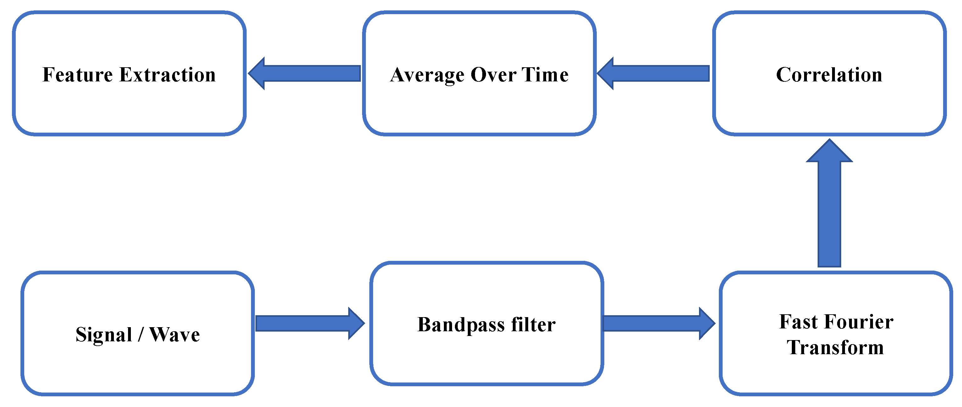
3.1. DEMON Processing

DEMON stands for the detection of envelope modulation on noise. This processing technique is accessible for the passive detection of submerged objects. This analysis is based on the statement that the pressure signal’s time-domain modulation can be recognized from the fast Fourier transform of the bandpass filtered sonar signal [63]. DEMON analysis, a narrowband analysis, is used to furnish the propeller characteristics [6]. This processing technique permits separating the cavitation noise from the overall signal spectrum and predicting the number of shafts, the rotation frequency, and rate of the blades. This technique gives enough information about the target propeller, and it can be used for target detection purposes [65]. The limitation of this technique lies in selecting a noise band, which requires good operating skills. Additionally, low noise immunity is another drawback of this method. The output of DEMON processing can be visualized in DEMON gram, which is a time-frequency spectrum spectrogram. Figure 3 shows the block diagram of DEMON processing. This analysis involves the following procedures:

• Selection of direction of interest
• Bandpass filtering to remove the cavitation frequency range of overall signal
• Squaring of the signal
• Normalizing the signal to reduce the background noise and to emphasize the target
• Using STFT to the normalized signal

3.2. Cyclo-Stationary Processing

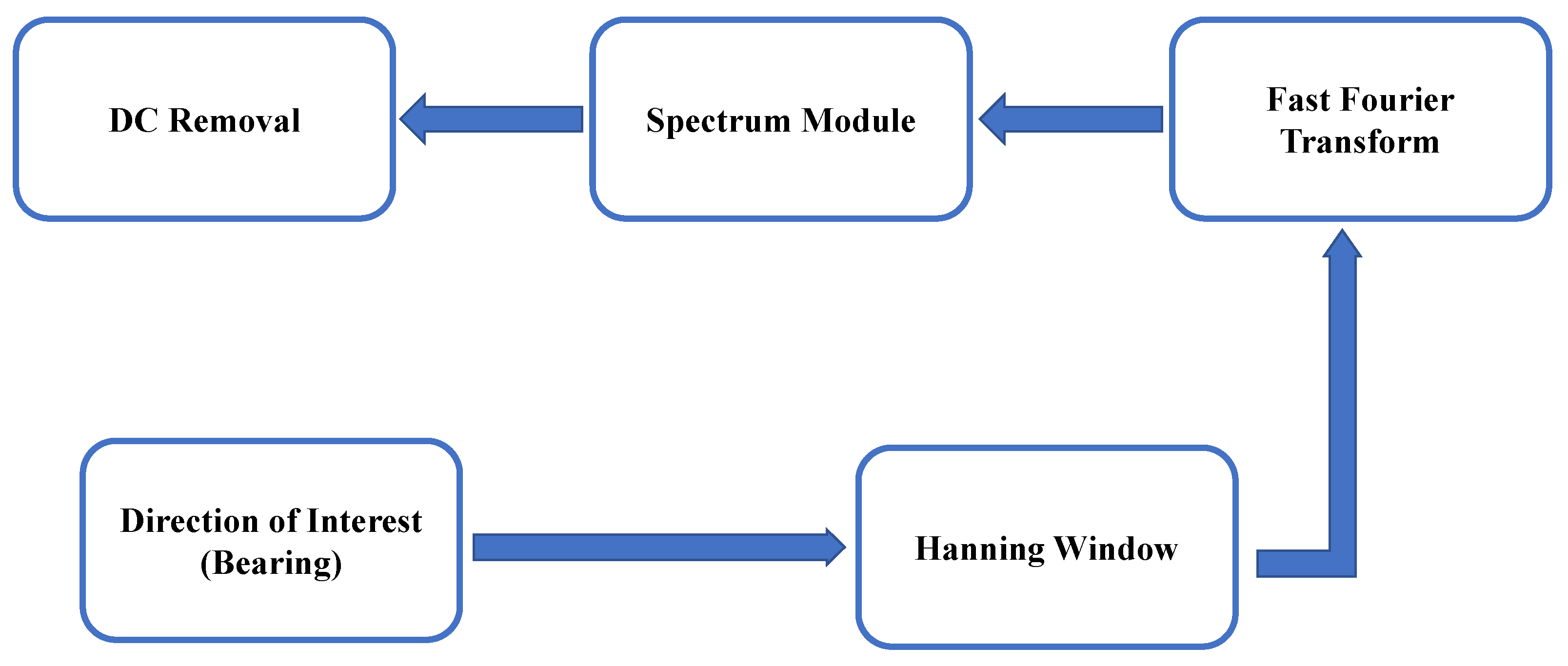
A cyclo-stationary signal contains time-varying statistical parameters with only or many periodicities. The idea of cyclo-stationarity is used in many real-world practices like detection of propeller noise in passive sonar. This technique overcomes the limitation of the DEMON processing technique by eradicating the pre-filtering requirement. It also offers enough enhancement in the case of noise immunity [63]. Cyclo-stationary processing concentrates on the frequency vs. cyclic frequency spectrum called the cyclic modulation spectrum (CMS). The main advantage of cyclo-stationary processing is that noise does not exhibit cyclo-stationarity, and the spectral correlation density of noise decreases to null for every non-zero value of cyclic frequency. Another critical property of cyclo-stationary signals is that they are easily detachable from other interfering signals. Even at low SNR, the CMS remains unchanged. Figure 4 shows the block diagram of cyclo stationary processing.

3.3. LOFAR Analysis

LOFAR stands for low-frequency analysis recording. LOFAR, a broadband study, predicts the target machinery’s noise vibration by providing the machinery noise to the sonar operator. The LOFAR analysis enables the operators can visually identify the frequency information of target machinery on the sonar wave data. This analysis, based on spectral estimation, supports the detection and classification of targets [66]. The signal to noise ratio (SNR) is low due to the discreteness of the sources. The narrowband component of signals provides an image of frequency vs. time, commonly known as lofargram. By characterizing the spectral lines on a lofargram, the acoustic source of sound can be determined [67]. By watching a waterfall-like lofargram, the operator can detect the tonal components [68]. The block diagram of this analysis is shown in Figure 5. LOFAR analysis involves the following steps:

• Selection of direction of interest
• Incoming signal processing with Hanning window
• Further processing of the resulting output with FFT

Again, for sonar images, pre-processing is the basis and an essential part of image recognition. Image preprocessing mainly consists of image denoising and enhancement. The function of sonar image preprocessing should be maximized to eliminate the effect of any kind of noise and reduce the impact of noise on the target area, and at the same time, enhance the actual target image in the water and parts of interest. The sonar image’s background noise is classified into three categories: reverberation noise, environmental noise, and white noise. The image denoising methods mainly consist of a self-adaptive smooth filtering method, median filtering denoising method, neighborhood averaging method, and wavelet transformation denoising methods [69]. One or more methods can be chosen according to the characteristics of the noise.

4. Deep Learning-Based Approaches for Sonar Automatic Target Recognition

Deep learning, a subdivision of ML, is based on artificial neural networks and inspired by the performance of human beings’ cerebrum cells called neural structure. In deep learning, it is unnecessary to instruct everything. It permits computational models composed of multiple processing layers to study data representations with different levels of abstraction. DL structures work with unstructured and structured data and perform automatic feature extraction without manual effort, and they have drastically upgraded the state-of-the-art in different fields, including automatic sonar target recognition [27,70].

DL algorithms can be grouped into supervised, semi-supervised, unsupervised, and reinforcement learning. A supervised learning approach is built on training a model with the correctly categorized data or labels to predict the mapping function such that when the new data is fed to the architecture, it can effortlessly estimate the outputs. Unsupervised learning functions for an unsupervised dataset, and it can study and establish information without providing loss signals to assess the probable solution [71]. Moreover, the semi-supervised learning approach conquers the limitations of unsupervised and supervised approaches by using a supervised learning approach to make the finest prediction for unlabeled data by using the backpropagation algorithm unsupervised learning approach to find and learn the pattern in the inputs to make the finest prediction. This algorithm uses only a small set of labelled data [72]. Again, one of the widely adopted techniques of deep learning is transfer learning. A transfer learning algorithm is a tool with a supplementary information source apart from the standard training data: knowledge from one or many relative tasks. Machine learning and deep learning methods work proficiently when the data is enormous in quantity. Nevertheless, having an enormous amount of data is unfavorable in real-world practices. Transfer learning resolves the issue of insufficient training data [73,74].

The aforementioned and numerous other pros of DL-based techniques attract the researchers to use these algorithms ubiquitously in almost all the fields. Image, speech and text recognition, object detection, pattern recognition, fault, and anomaly detection are fields DL methods have performed well. In sonar ATR, the DL models have shown their excellency with higher accuracy and reliability. The next section explains the DL models employed in sonar signal processing, and

Table 1. The tabular analysis of the deep learning algorithms reviewed in this article.

A. R. 1	Method	Other Details	Remarks
[68]	11-layer CNN Kernel of 3 × 1 in the first 10 layers, and the kernel of the input-height × 1 in the last layer	LOFAR analysis as preprocessor A Sonar simulator is used to generate the data	92.5% of precision and 99.8% of recall
[48]	4-layer CNN	Data augmentation tool: Flipping and rotation	Cross-entropy loss function Input batches size: 20
[80]	Faster R-CNN StyleBankNet is used to synthesize the noise characteristics of sonar images	Conversion of the images to grayscale was done for data augmentation	Input size: 32 × 32 × 3 SoftMax is used in the classification layer
[12]	Efficient CNN with an encoder and a decoder network The encoder network consists of 4 encoders made up of residual building blocks and convolutional blocks The decoder network consists of four decoders, using max-pooling operation	SSS data accumulated by dual-frequency SSS Shark-S450D in Fujian, China Used LabelMe to label images	Input size: 240 × 240 The method realizes the best trade-off between effectiveness and efficiency
[82]	CNN for object detection in FLS	Captured FLS images from their water tank	Input image size: 96 × 96 99.2% accuracy
[84]	Outputs from CNN and FCN on LiDAR data and sonar images are processed with K-Means clustering DBSCAN methods	Both the datasets were introduced to SSD to alter the data type from 3D point cloud to image.	Input image size: 28 × 28 Highest accuracy 100%
[86]	3- layer SAE KL and MSE for measuring reconstruction error	LOFAR analysis as preprocessor	87.0% detection accuracy
[87]	CNN-based 6-layer DAE Images captured with audible lens-based multi-beam sonar	Images were cropped to 64×64 size	13,650 images were trained
[88]	Computational and energy efficient CDA-TBD method 4 convolutional and 4 deconvolutional layers	ReLU as activation function CDA was trained with error back-propagation	Yielded an excellent trade-off between recall and precision
[91]	3 hidden layer DBN algorithm to classify four dissimilar incomings of sonar targets with multi-aspect-based sensing FrFT-based features	Ray-tracing method was used to synthesize active sonar incomings	Average accuracy of 91.40% was obtained
[47]	Deep competitive belief network-based algorithm to resolve the tiny-sample-dimension issue of underwater acoustic target detection	The training and testing data was taken from the South China Sea at a	The system achieved a 90.89%
[92]	cGAN-based realistic image generation system The generator and discriminator network models used in this project are CNN-based architecture	The model is tested in a fish container carrying thousands of sardines	The color distribution matching property, pixel-wise MSE, and structural similarity indices are used as the evaluation matrices
[87]	GAN-based algorithm to produce a genuine sonar segment or images to use sonar signals better The generator is a U-Net architecture consisting of 15 layers, and the discriminator architecture was a CNN comprised of four convolutional layers	Sonar image simulator-based on the ray-tracing technique was implemented GAN-based style transfer method transformed simple images into genuine sonar images	Generator uses skip connection as well
[95]	cGAN-based method to transform low-resolution sonar images to high resolution	Two-part work: using simulated data and using measured sonar data	Satisfactory result
[96]	Markov conditional pix2pix method to generate SSS images	The actual SSS data used in the research is obtained with a marine sonic sonar	Synthetic data were produced 18 times quicker than actual collection speed
[97]	GAN-based approach to improve the usability and adaptability of ATR procedures in the new atmosphere	The synthetic contacts were created on ray tracing a 3D—CAD model into the actual side-scan seafloor	Average accuracy of 97% for synthetic images and 70% for refined images was obtained
[100]	RNN-based algorithm for distinguishing tiny human-made objects in orders of medium sector-scan sonar imagery	The sonar images were accumulated with a sonar structure mounted beneath a vessel	Probability of 77.0% detection at an average false-alarm proportion of 0.4 per image was obtained

¹ A.R.: Article Reference.

shows the tabular analysis of those models

4.1. Convolutional Neural Networks

LeCunn first proposed convolutional neural networks (CNNs) for image processing [75]. Convolutional neural nets have enormously enhanced the productivity and effectiveness in computer vision, natural language processing, text and speech recognition, object detection, medical prognosis, etc., with the rise in GPU memory and manufacturing. Certainly, CNNs are one of the utmost DL structures, making them used extensively within computer vision. The period of deep convolutional neural nets has featured and instantly replaced the out-of-date classification and acknowledgment methods within a short duration, after the significant overview of AlexNet [76]. With special convolution and pooling operations, CNNs perform parameter sharing, enabling these architectures to run in any device universally. The multilayer structure of CNN can automatically study several level characteristics, which are used to categorize the image class. Because of the computational efficiency of CNNs and their self-learning capacity, they provide robust and efficient performance in image processing; thus, they are used these days ubiquitously [77]. The use of CNNs in sonar ATR for object detection or classification has been practiced recently. Some of the published works for detecting and classifying sonar targets with a CNN architecture have been explained in the subsequent section. Figure 6a shows the typical 2-D CNN-based network structure. A 1-D-CNN has also been developed for dealing with 1-D data. The 1-D-CNN is an improvement on the 2-D-CNN and is more efficient for specific applications that deal with 1-D signals because the forward propagation (FP) and backward propagation (BP) are simple array operations rather than matrix operations. 1-D-CNNs, in other words, in Conv1D, the kernel slides along one dimension and the relatively flat structure of 1D CNNs make them suitable for learning challenging tasks with 1D signals and for real-time use. Figure 6b shows a typical structure of a 1D CNN. Recent works have shown that compact 1D CNNs perform well in applications that rely on 1D data; applications of 1D CNNs include analysis of 1D sensors and accelerometer data, natural language processing, and speech recognition [78,79].

The research article [68] talks about recognizing tonal frequency in a Lofargram with the use of CNN. The authors divided a Lofargram into tiny patches, and a convolutional neural network is used to predict either the patch is from the tonal frequency or not. With this structure, 92.5% of precision and 99.8% of recall was obtained, taking 0.15 seconds of inference batch processing time at a particular time frame. For the creation of Lofargram, the beam-formed time-domain wave data is filtered by a particular window and transformed using STFT into frequency-domain data, which is further squared and then combined for a short time to confirm that each frequency bin signifies the spectral power. Then the normalization technique is implemented to control the background sound and to emphasize the leading frequency information. A Sonar simulator is used for the generation of data. An 11-layer CNN is used for classification where the kernel of 3 × 1 is used for the first ten layers, and the kernel of the input-height × 1 is used in the last convolutional layer. This is done to collect time-domain information to a single height and decrease neural network parameters prior to the fully connected layer. They used sigmoid as the activation function.

In [48], a DL-based method to classify target and non-target synthetic sonar aperture (SAS) images is proposed. A fused anomaly detector is used to narrow down the pixels in SAS images and extract target-sized tiles. The detector produces the confidence map of the same size as that of the original image after calculating a target probability value for all pixels based on a neighborhood around it. The confidence map permits only the region of interests (ROIs) neighboring as the most expected pixels to be considered by the classifier. The deep learning architecture used is a 4-layer CNN. After convolution and max-pooling layers, a fully connected layer with a dropout is fed into a final two-node output layer defining a target and false alarm forecast values. Cross-entropy is used as the loss function for input batches of size 20 for 2000 epochs. They implemented a global location-based cross-validation method for network performance validation and a fold cross-validation technique for validation purposes. Flipping and rotation techniques were used as the data augmentation tool. To further improve classification accuracy, the classifier fusion method to approximate a tile’s true-confidence rank beyond a single structure is used. The experimental results for the proposed system are quite promising. The Choquet classifier, which continues surpassing the detector during all false alarm rates, also improved the result of the individual four networks.

An end-to-end style-transfer image-synthesizing generation method in the training image preparation phase is proposed to solve underwater data scarcity [80]. The proposed method takes one channel depth image from a simulator to provide various aspects like scale, orientation, and translation of the captured data. A thorough evaluation was performed using real sonar data from pool and sea trial experiments. The authors captured a base image for the synthetic training dataset from a simulated depth camera in the UWSim. StyleBankNet is adopted to synthesize the noise characteristics of sonar images acquired in an underwater environment. This network simultaneously learns multiple target styles using an encoder, decoder, and StyleBank, which consists of multiple sets of style filters, each set representing the style of one underwater environment. The StyleBankNet uses two branches, the autoencoder branch and stylizing branch, to decouple styles and contents of sonar images and train the encoder and decoder to generate output as close as possible to an input image. The dataset for training the StyleBankNet consists of a content set composed of base images and multiple style sets. The network architecture applied for object detection is faster region CNN. 3-layer region proposal network is used in which the input of 32 × 32 × 3 is fed. SoftMax is used in the classification layer. For the augmentation, the authors converted the images to grayscale and their inverted image in the form of general one-channel sonar images.

In [12], an efficient convolutional network (ECNet) to apply semantic segmentation for SSS images is proposed. The network architecture comprises an encoder network, for capturing context, a decoder network, for reestablishing full input-size resolution feature maps from low-resolution maps for a pixel-wise organization, and a single stream DNN with numerous side-outputs to enhance edge classification. The encoder network consists of four encoders made up of residual building blocks and convolutional blocks for extracting feature maps. Similarly, the decoder network consists of four decoders, using max-pooling operation on their input feature maps. Three side-output layers, in which in-depth supervision is performed, are placed behind the first to the third encoder. A 1 × 1 convolution layer follows each of the last layers in the first to the third encoder in the side-output component, and next, a deconvolution layer up-samples the activation maps to recover the native size. The side-scan sonar data are accumulated by dual-frequency SSS (Shark-S450D) in Fujian, China. As the data pre-processing, the middle waterfall was removed, and bilinear interpolation on the raw data was performed. The authors made use of LabelMe [81], an image notation tool created by MIT, to physically label images, which are further cropped at the size of 240 × 240. The train-test ratio was 0.7:0.3, and 20% of the training data was used for the validation set. Stochastic gradient descent (SGD) was used for optimizing loss function with the global learning rate of 0.001. The proposed method was juxtaposed with U-Net, SegNet, and LinkNet. The result shows that the proposed method was much faster and contains fewer parameters than the other models, and it realizes the best trade-off between effectiveness and efficiency.

In [82], CNNs were employed for object detection in forward-looking sonar (FLS) images. They captured FLS images from their water tank, comprising several kinds of debris objects, with an ARIS Explorer 3000, at the 3.0 MHz frequency setting with a variation of 1 to 3 meters. They used 96 × 96 sized images as the input to their CNN model. Mini-batches of batch size 32, an initial learning rate of 0.1, SGD, and Adam optimizers were other network parameters. The train-test ratio was 0.7:0.3, and the number of classes to be classified was 10, and SoftMax was used as a classifier. The authors presented that their model outperforms template matching methods by attaining 99.2% accuracy. They also showed that their model requires fewer parameters and, being 40% faster, permits real-time applications. The same authors in [83] proposed a model to detect objects and recognize them in FLS images. After fine-tuning an SVM classifier trained on the shared feature vector, the accuracy obtained was found to be 85%. The authors claim that their detection proposal method can also detect unlabeled and untrained objects, have good generalization performance, and be used in any sonar image.

In [84], two clustering procedures are applied to both 3-dimensional point cloud LiDAR data and underwater sonar images. The outputs from using CNN and fully convolutional networks (FCN) on both datasets are processed with K-Means clustering and density-based spatial clustering of applications with noise (DBSCAN) methods to eliminate outliers, identify and group meaningful data, and progress the result of multiple object detections. In this research, the FCN was employed to train and test the segmentation on the underwater sonar image dataset, which was then converted to pixel data representing a matrix comprising two values, x, and y, in the coordinating elevation position. Both the datasets were introduced to spherical signature descriptor (SSD) to alter the data type from 3D point cloud to image. These image data were then fed to the CNN model and were further classified into five different classes. The CNN architecture used was with the repetitive convolving and the max-pooling layers. The input size of image data was 28 × 28 pixels. In the preceding layers, the kernel size was 5 × 5, while in the latter layers, the size was 3 × 3. The activation function was ReLU in the convolution layers and the SoftMax in the last layer. The highest accuracy of 100% was obtained with the proposed model.

4.2. Autoencoders

An autoencoder, a kind of unsupervised neural structure, decreases dimensions or finds feature vectors [1]. Autoencoders are widely adopted algorithms that are programmed to reproduce their input to output. The input and output layers consist of a hidden layer h, which outlines a code used to represent the input. The architecture contains two parts:an encoder, mapping input into the code $h=f\left(x\right)$, and a decoder, producing a reconstruction $r=g\left(h\right)$ [85]. Let, $x$ and $h$ representing the input data vec $\left\{x_1,x_2,\dots ,x_n\right\}$ and the vector in the hidden layer $\left\{h_1,h_2,\dots ,h_n\right\}$ respectively. Again, $r$ is the outcomes of the output layer $\left\{r_1,r_2,\dots ,r_n\right\}$ and it also signifies the reconstructed data vector simultaneously. Taking the MSE between the original input data and output as a loss function, the ANN copy the input as the final output. After this, the network is trained, keeping only the encoder part and removing the decoder one, thus making the encoder’s output a feature representation fed to following-stage classifiers [27].

Much research has been done using an autoencoder to detect and classify sonar targets and objects. The pioneering work was done by V.D.S. Mello et al. [86]. The authors implemented stacked autoencoders (SAE) for detecting unidentified incoming patterns in a passive sonar system. For novelty detection, all four target groups in the dataset were used to distinguish the new class. Hence, an unidentified group was introduced to the detector after the identified group training process. They implemented LOFAR analysis as the preprocessor. The Lofargram obtained was fed as the input of a 3-layer SAE. Two merit figures were used to measure each autoencoder’s reconstruction error in the pre-training step: Kullback-Leibler divergence (KLD) and MSE. KLD computes a quasi-distance between probability density functions predicted for the original dataset and their renovation. The Brazilian Navy provided the dataset used in this work. The dataset was collected with a unidirectional hydrophone placed close to the bottom of the range. The incoming signals were digitalized with a sampling frequency of 22,050 Hz. To decrease the sampling frequency to 7.35 kHz, a decimation was implemented to successive blocks of 1024 points. With the threshold value equals to 0.5, the novelty detection accuracy using SAE was obtained to be 87.0%.

In [87], the authors proposed a CNN-based sonar image noise limiting method with the denoising autoencoder (DAE) system. The audible lens-based multi-beam sonar was used for taking imageries in the clouded water environment. The network structure used is a 6-layers structure, in which there are 3 convolution and 3 deconvolution stages. There are 32 depths in the first layer, 64 in the second 128 in the third layer. The sonar images are cropped to 64 × 64 size, followed by an artificial injection of gaussian-noise, then fed to the input layer. Finally, the model is trained with the cropped original data. In the proposed study, the total number of images trained is 13,650. The dataset was created by taking pictures from the actual sea area with the help of AUV Cyclops. The objects like bricks, cones, tires, and shelters were placed on the sea surface, and the images were taken. Additionally, the photographing was performed in a moving situation also. The proposed method worked efficiently for reducing noise.

In [88], a computational and energy-efficient pre-processing stage-based method to correctly distinguish and track submerged moving targets from the reflections of an active acoustic emitter was proposed. This research is conducted employing a deep convolutional denoising autoencoder-track before detecting (CDA-TBD), whose output was then provided to a probabilistic tracking system based on the dynamic programming known as the Viterbi algorithm. For the network architecture, the autoencoder was comprised of four convolving layers consisting of 24, 48, 72, and 96 kernels of dimension 4 × 4, 6 × 6, 8 × 8, and 12 × 16, respectively. The first three layers were followed by pooling layers, with pool size 1 × 2 and stride 1 × 2. Convolutional or encoding layers are followed by four deconvolutional layers of the equivalent dimensions using the nearest neighbor as an up-sampling function. For the activation function, ReLUs were used in all layers. The last layer using logistic units was connected as a concluding stage to generate output values in the range of zero and one. Figure 7 shows the structure of a convolutional denoising autoencoder used in this research. Here, the noisy time-distance image is introduced as an input, which is further treated by a pile of convolving layers. The decoder used the complex features detected by the convolving layers to generate a denoised time-distance matrix. The CDA is trained with error backpropagation. The results showed that despite the poor reflection patterns from the target and low signal to clutter ratios, the proposed system yielded an excellent trade-off between recall and precision, exceeding the function of fully probabilistic methods at a significantly lesser computational complexity, and also allowed for an additional precise fine-grained tracking of the target path. Furthermore, the results also showed that the method effortlessly scaled to situations featuring several targets.

4.3. Deep Belief Networks

Deep Belief Networks (DBNs) are the network models comprising of several middle layers of Restricted Boltzmann Machine (RBM), where all the RBM layers are connected with the preceding and the subsequent layers. These networks were proposed for the first time in [89]. These layers do not have any intra-layer connection, and the last layer is used for the categorization. Unlike other architectures, all the layers of DBN learn the entire input. The deeper deep belief networks address the subject by representing several characteristics of input patterns hierarchically with MLPs getting trapped at local optima. Moreover, they also optimize the weights in all layers. This method of solving the problem involves making the optimal decision in all layers in the order, eventually obtaining a global optimum [27].

The greedy learning systems begin with the first layer and keep going, fine-tuning the generative weights. At this time, the DBN layers are trained one at a time, i.e., layer-by-layer basis learning is performed. As a result, all the layers gain unique data. All the layers of DBN have a double role, except for the first and last layers. The dual role includes serving as the hidden layer to the preceding nodes and visible or an input layer to the next ones. This structure can be referred to as an architecture made up of single-layer networks, which is able to resolve issues like low velocity and the overfitting phenomena in DL. The DBN architecture used in [47] is shown in Figure 8. In addition to using these networks in clustering recognizing and generating images, motion-capture data, and video sequences, they are also used in sonar ATR systems for detection and classification [90]. Some available works are described below.

In [91], an algorithm to classify four dissimilar incomings of sonar targets with multi-aspect based sensing, fractional Fourier transform (FrFT)-based features, and a 3-hidden-layer DBN was proposed. The author synthesized the active target echoes based on the ray-tracing method with a target prototype having three-dimensional highlight distributions. The fractional Fourier transform (FrFT) was implemented to the synthesized target echoes in order to obtain a feature vector. Active sonar incomings from target objects were synthesized based on the ray-tracing method for three-dimensional highlight systems. The authors compared their model with the conventional backpropagation neural network (BPNN) method. The other details include - the water depth was set to 300 m, the distance between the target and sensor is 5000 m, monostatic mode of transmission, active sonar returns for each target were generated by varying its aspect from 0 to 360 degrees by 1-degree increment. The linear frequency modulation (LFM) pulse interval and sampling frequency were set to 50 ms and 31.25 kHz. The central frequency and bandwidth of the LFM signal were 7 kHz and 400 Hz. The α parameter of FrFT was set to 0.9919. The feature vector was acquired by splitting the FrFT domain into 100 equivalent bands and computing each band’s energy. The feature extraction procedure led to 100th-order FrFT-based features that adequately represent shape changes and possess discrimination ability. The average accuracy of 91.40% was obtained using DBN, whereas the 100-24-4 structure BPNN model gave 87.57% accuracy.

Similarly, in [47], the authors proposed the deep competitive belief network-based algorithm to resolve the tiny-sample-dimension issue of underwater acoustic target detection by learning features with additional discriminative information from labelled and unlabelled objects. The four stages in the proposed system are: pre-training the standard restricted Boltzmann machine for the parameter initialization using a massive amount of unlabeled data, grouping the hidden units according to the categories for providing original clustering system for competitive learning, updating the hyper-parameters to achieve the clustering task by the use of the competitive training and backpropagation algorithm, and then building a deep neural network (DNN) by implementing layer-wise training and supervised fine-tuning. The training and testing data was taken from the South China Sea at a sampling frequency of 22.05 kHz using an omnidirectional hydrophone located at 30 m beneath the sea level. The unlabelled data in the dataset contains oceanic ambient noise and emitted noise from the vessel, whereas the labelled data contains emitted noise from two groups of a vessel with label info, small boats, and autonomous underwater vehicles. Both the groups of targets were about 3.5 km far from the recording hydrophone and moved along the very same route at different proportions. It was made sure that no vessels existed in a radius of approximately 10 km to avoid interference. The results showed that the system achieved a 90.89% classification, which was 8.95% higher than the accuracy attained by other compared approaches.

4.4. Generative Adversarial Networks

Generative adversarial networks (GANs) are DNN architectures composed of two networks challenging for one against the other. These neural nets can create or make new content. Working with arbitrary inputs, they create something on the output. [79]. Figure 9 shows a GAN architecture used in [92]. First introduced by Ian Goodfellow and other scientists in [93], these networks consist of the discriminator, D, and the generator, G, playing the two-player minimax game [93] with a value function

$$Mi{n}_{G}Ma{x}_{D}V\left(D,G\right)=E_{x~pdata\left(x\right)}\left[\log D\left(x\right)]+E_{z~pz\left(z\right)}\right[\log (1-D\left(G\left(z\right)\right))]$$

(2)

The generator tries to produce samples having an equivalent probability distribution as the actual training dataset. The discriminator, on the other hand, is responsible for identifying whether the input is from the actual dataset or the generator and guiding the generator over the backpropagation gradient to create a more realistic sample data. Throughout this two-player min-max game, the generator outputs a fake sample taking in impulsive noise as input. The discriminator processes the training dataset sample as the input for half of the duration and takes in the generator’s reproduced sample, G_Sample, as an input for the next half.

The discriminator is skilled in maximizing or optimizing the distance between classes and distinguish between the real image from the training dataset and the generator’s reproduced samples. Hence, the generator should make the generated probability distribution and the real data distribution as close as feasible so that the discriminator cannot choose between the actual and the fake sample. Therefore, in this adversarial process, the generator improves itself to learn the real data distribution, and the discriminator also improves its feature learning capacity. Finally, the training reaches Nash equilibrium, where the discriminator cannot isolate two distributions, i.e., D(x) = ½. There are many studies [49,94] carried out for finding this equilibrium. [93], alike in other fields, the implementation of generative neural networks is growing in sonar signal systems too. Numerous works using GAN are available for the detection and classification of various underwater sonar targets. Some are described in the next section.

In [92], a conditional generative adversarial network (cGAN)-based realistic image generation system was proposed, in which the model learned the image-to-image transformation between optical and sonar images. The model is tested in a fish container carrying thousands of sardines. The image data used in the system were captured using an underwater camera and a high-accuracy imaging sonar. The authors created nightly images by steadily darkening the captured camera image with artificial noise and using the resultant images and the sonar images as input. The model is then trained to produce authentic daytime images from the input. The color distribution matching property, pixel-wise MSE, and structural similarity indices are used as the evaluation matrices for comparison. The generator and discriminator network models used in this project are CNN-based architecture. The inputs are passed through a 3 × 3 convolution layer and concatenated, and through seven down-sampling (4 × 4 deconvolutional) and seven up-sampling (4 × 4 convolutional) CBR (Convolution-BatchNorm-ReLU) layers in the generator network. Moreover, the dropout layers are added in the decoder part. The last 3 × 3 convolutional layer yields an image. To record high-frequency info, the discriminator configures a PatchGAN model, which estimates the architecture at the scale of local patches to label patches in the image. The discriminator’s ultimate output is determined by making an average of the probability of all patches produced by the last 3 × 3 convolutional layers. The size of the patch for the discriminator network was set to 8.

M. Sung et al. proposed an algorithm to produce a genuine sonar segment or images to better use sonar signals [87]. The proposed method contains two steps: sonar image simulation and image transformation with the help of GAN. First, the authors employed the sonar image simulator-based on the ray-tracing technique by calculating the transmission and reflection of sound waves. The simulator simulates images containing semantic information such as highlighting and shadowing through simple calculations. The GAN-based style transfer method transformed these simple images into genuine sonar images by putting on noises or changing actual sonar images into the simple images via denoising and segmentation. The authors adopted the pix2pix model. The generator of GAN is a U-Net architecture consisting of 15 layers. The generator could augment or eliminate the noise preservatives of the input image using a feature map. Skip connection, via which the decoder imitates activation map from previous layers, was another characteristic of a generator. The discriminator architecture was a CNN comprised of four convolutional layers. The discriminator was used to observe input images by splitting them into tiny patches. The outputs of the proposed algorithm showed an excellent resemblance to the ground truth.

The authors proposed a conditional GAN (cGAN)-based method to transform a low-resolution sonar image to its high-resolution counterpart using the image-to-image translation technique [95]. The cGAN learns an input-to-output mapping and a cost function to train the mapping. They tested the proposed method by training a cGAN on simulated data. The method is analyzed using measured synthetic aperture sonar (SAS) dataset collected by Svenska Aeroplan Aktie Bolag (SAAB). The work in this paper is divided into two parts: one part using simulated data and another part using measured sonar data. Simulated SAS data is generated at the signal level for the proof of concept. Two kinds of datasets were created where each scene in an image of the first dataset (say A) corresponds to that of an image in another dataset (say B). A holds sonar images created from a short array of 50 elements. The dataset B holds the corresponding sonar images for a more comprehensive array with 100 or more elements. The spacing between the elements is always the same, so a 100-element long array is twice the 50-element array. This research showed that it is feasible to go from a low-resolution sonar image produced from a (short-array) to its high resolution (long-array) counterpart with simulated data.

Similarly, in [96], an algorithm for producing authentic SSS images of full-length missions, known as Markov conditional pix2pix (MC-pix2pix), was proposed. Synthetic data were produced 18 times quicker than actual collection speed, with full operator control over the topography of produced data. To validate the method’s utility, the researchers provided numerical results in 2 extrinsic assessment tasks. The synthetic data was almost impossible to differentiate from actual data for specialists. The actual SSS data used in the research is obtained with a marine sonic sonar, whose across-track resolution is 512 pixels. The speed of the vehicle is 1 m per second and produces around 16 pings per second. The vehicle’s turning used to create distortions in the images, and the system which produced synthetic imagery was anticipated to create identical distortions. The system accounted for these alterations using the desired vessel’s attitude information (roll, yaw, and pitch). Usually, the yaw information is only delivered by the collected training dataset, but the proposed method can incorporate pitch and roll data. Sonar scans were processed to 464 × 512 dimensions to create a training dataset. This model was trained on a comparatively small dataset of 540 images and their identical semantic maps.

To improve the usability and adaptability of ATR procedures in the new atmosphere, a GAN-based approach is proposed in [97]. This method was used to enhance simulated contact into actual SSS images. The synthetic contacts were created on ray tracing a 3D computer-aided design (CAD) model at a particular place into the actual side-scan seafloor. A real shadow was created by calculating the elevation map of the seafloor. The elevation was computed by recognizing coupled shadows and highlights, which were the elevations connected to the neighboring shadow. Then, the synthetic contact appearance was refined using CycleGAN. The average accuracy of 97% for synthetic images and 70% for refined images was obtained. The simulator, in the proposed method, can insert 100 simulated contacts in approximately 20 s. The simulator could insert 100 simulated contacts in ≅ 20 s.

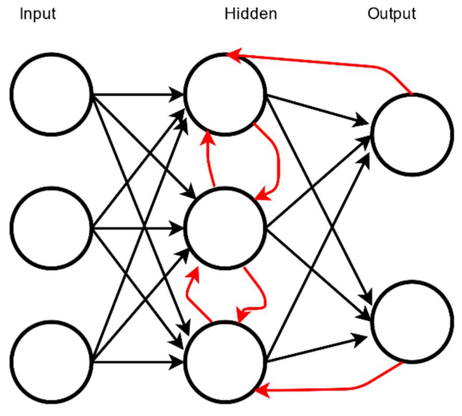
4.5. Recurrent Neural Networks and Long Short-Term Memory

Recurrent neural networks (RNNs) are artificial neural networks that permit previous outputs to be operated as inputs though they have hidden stages. These networks recall the previous states, and their choices are inclined to their learning from the earlier stages. Hence, RNNs continually process the input [98]. Long short-term memory (LSTM) networks were introduced to solve the gradient exploding or vanishing problem caused by RNN. Additionally termed as the cell network, LSTM takes the input from the earlier and present stages. RNNs are used widely in speech and text recognition, natural language processing, and sonar ATR systems. Figure 10 illustrates the architecture of the LSTM network used in [99].

S.W. Perry and Ling Guan presented an algorithm for distinguishing tiny human-made objects in medium sector-scan sonar imagery orders accumulated with a sonar structure mounted beneath a vessel [100]. Object detection was done up to 200 m from the moving vessel. The authors began by approximating the movement of the vessel on the basis of tracking objects on the seafloor. With this estimation’s help, the temporal cleaning of imagery was done by normalizing many pings after compensating for the vehicle’s motion. In the resulting image order, the appearance of targets resting on the seafloor was improved, and clutter noise was minimized. The working of the detector is in two steps. In the first step, it was expected to identify probable objects of interest. The second stage involved tracking those objects identified in the first stage and supplying the sequence of feature vectors to the classifier. RNN was used as the final detection classifier. The comparison of a result obtained using RNN and that of using non-RNN was done. The proposed method achieved a probability of 77.0% detection at an average false-alarm proportion of 0.4 per image.

5. Transfer Learning-Based Approaches for Sonar Automatic Target Recognition

As mentioned before, the deep learning-based architectures perform proficiently with the enormous amount of data. However, getting a tremendous amount of data is not always feasible in a real-world scenario. The transfer learning method was proposed for solving this scanty data problem. Transfer learning is an essential and widely accepted method for solving insufficient training data in machine learning [101]. Recently, deep transfer learning approaches are being widely practiced. Some deep transfer learning strategies used in sonar ATR are summarized and overviewed in the following section, and

Table 2. The tabular analysis of the transfer learning-based DL algorithms reviewed in this article.

A. R.	Method	Other Details	Remarks
[102]	Transfer learning-based CNN method to detect submerged human body GoogleNet was used as the network architecture The researchers developed a model for classifying the multi-beam sonar images within the noises like scattering and polarization	3 sets of data were used Data augmentation: added background and polarizing noises and the use of inversion technique	Used dummy as the submerged body The best accuracy of GoogleNet was 100%
[33]	Deep transfer learning-based method for object detection for SSS imagery Using a pre-trained CNN, the authors trained the newly produced YOLO model with a small training dataset and tested it to detect and classify sonar images	a systematic transfer learning approach was employed to detect objects or anomalies in sonar images	The confidence probability went up to 95% after training for 500 epochs

shows the tabular analysis of the methods implemented

In [102], CNN was implemented to detect a submerged human body for the underwater image classification. Here, the researchers developed a model for classifying the multi-beam sonar images within the noises like scattering and polarization. The authors used a clean and turbid water environment to collect sonar data of the submerged body. They used the dummy as the submerged body. Out of three datasets used, one set was taken in the Korea Institute of Robot and Convergence (KIRO) clean water testbed, and the other two sets were captured under turbid water conditions on Daecheon beach in Korea in 2017 and 2018, respectively. This water testbed’s maximum depth is about 10 m; a dummy positioned in a water depth of about 4 m was used to affect the submerged body. They used GoogleNet architecture for classifying two classes: body and background. As the preprocessor, they added background and polarizing noises to the original images, and the inversion technique is implemented to augment the training dataset. The pixel density of the images was also adjusted. TELEDYNE BlueView M900-90, which can rotate the sonar sensor at the angular gap of 5 degrees, was put on a gearbox to get useful underwater sonar images from several angles. The best accuracy of GoogleNet, which is 100%, was at level 3 of polarizing and intensity.

Dylan Einsidler, in his M.S. thesis [33], proposed a deep learning-based transfer learning method for object detection for side-scan sonar imagery. In this research, a systematic transfer learning approach was employed to detect objects or anomalies in sonar images. A pre-trained CNN was employed to learn the pixel-intensity based features of seafloor anomalies in sonar images. Using this transfer learning-based DL approach, the authors trained the newly produced ‘you only look once’ (YOLO) model with a small training dataset and tested it to detect and classify sonar images. A Hydroid REMUS-100 AUV was used to obtain side-scan sonar data for collecting training and testing data used in the experiments. The data used in this thesis are from several real-sea experiments conducted at SeaTech Oceanographic Institute of Florida Atlantic University. The authors used the TinyYOLO model. The learning rate was set to 0.001, the momentum was set to 0.9, the decay was set to 0.0001, the batch size was set to 64 images, and the class threshold is 0.1. The confidence probability went up to 95% after training for 500 epochs.

6. Challenges in Sonar Signal and Automatic Target Recognition System

The detection and classification of underwater minerals, pipelines and cables, corals, and docking stations is essential. However, the sonar data have characteristics such as non-homogenous resolution, speckle noise, acoustic shadowing, non-uniform intensity, and reverberation, making it hard to process. Other problems include dual object detection problems, acoustic sonar targets’ appearance in various sizes and aspect ratios, and class imbalance [103]. The most challenging thing one encounters while working with sonar signals is the marine environment. Due to the very low bandwidth of the medium, underwater communication is very poor. Underwater sound propagation is a complex phenomenon that depends on temperature, pressure, and water depth. The quantity of salt in water is also responsible for the change in underwater sound propagation speed. The surface and underwater temperature difference cause a change in the refractive index (R.I.), resulting in the sonar signals being refracted off surface and depth without reaching the target. Again, scattering is another challenge by small underwater objects, making the required object hard to be located due to interference.

The noisy nature of sonar imagery and the lack of sonar data availability make automatic target recognition in autonomous underwater vehicles a daunting task [33]. To capture sonar images and for new sonar-based methods to emerge, numerous underwater experiments should be performed. These experiments require plenty of time and resources despite using an unmanned underwater vehicle (UUV) [104]. The use of high-resolution sensors can improve sonar systems’ performances; however, these sensors are highly expensive.

Moreover, for many background pixels in the side-scan sonar image, the imbalanced categorization remains an issue. Side-scan sonar images contain undesirable speckle noise and intensity inhomogeneity. Again, some pixels in the images are weak; and some are discontinuous [12]. The detection of submerged mobile targets through active sonar is challenging due to the low reflection signature of such targets resulting in the low signal-to-clutter ratio [88]. Similarly, the use of traditional algorithms in sonar target segmentation takes up to several minutes to process one sonar image with a high number of false alarms. Again, most of the automatic target recognition techniques are tested on the data recorded in simple or flat seabed regions. As a result, these methods fail to perform well in complex seabed regions.

Additionally, the detection range is a misunderstood sonar coverage metric. Range detection ranking metrics are mostly irrelevant to performance prediction because the detection range is calculated for a set of propagation conditions, and the conditions are changed at mission time. Again, the conventional dedicated ships are being replaced by small, low-cost, autonomous platforms that can be easily used on any vessel. This leads to new acquisition and processing challenges as the classification algorithms need to be fully automated and run in real-time on the platform [105]. Additionally, regarding the underwater acoustic networks, the transducer’s narrow bandwidth response results in a limited frequency bandwidth for underwater communications. Therefore, the transmission potential of cognitive acoustics users is significantly limited by this hardware. Highly dynamic underwater channels call into question the reconfiguration of parameters [106].

7. Challenges Using DL Models for Sonar Target and Object Detection

Underwater sonar signals are abundant sources of information that help understand the phenomenon related to the sonar ATR system, thus helping the researchers track or detect the object of interest. The use of DL algorithms has provided high accuracy in almost every field. Despite the remarkable advances in sonar ATR with the help of DL algorithms and computer vision, the performance of these algorithms is still full of obstacles and has yet to gain broad acceptance. Though the DL algorithms’ numerous pros have encouraged the researchers to use DL algorithms to track and detect objects of interest in the sonar systems, these DL models have some limitations. Some of these hindrances relate to the practicality of the techniques, and some relate to the theoretical limits. The difficulties with deep neural networks are related to its architecture and training procedure. Despite the widespread literature on deep learning algorithms, they need prior knowledge regarding their architecture [107]. Multiple scales, dual nature, speed, data scarcity, and class imbalance make object detection challenging. In underwater object detection, further complications arise due to acoustic image problems such as non-uniform intensity, speckle noise, non-homogenous resolution, acoustic shadowing, acoustic reverberation and multipath problems [103]. The DL-based approaches are not well established for acoustic sonar target detection. The challenges using DL models for tracking, detection, and classification using sonar systems are listed below:

• DL models, when provided with vast data, perform well. Moreover, collecting vast amounts of sonar data for these algorithms to perform proficiently is a challenge as there are few open source databases. Datasets collected for Navy and military purposes are highly confidential and cannot be used by the common researchers.
• Training deep learning architectures is intensely computational and costly. The most sophisticated models take weeks to train using high-performance GPU machines and require considerable memory [108].
• DL algorithms require vast amounts of training data. Obtaining enormous data for sonar ATR is difficult due to the high cost and limited plausibility of real underwater tests for researchers to conduct. Though different simulation tools generate real-like data and augment data for better training, the simulated data lacks the same type of variability found in real data [33].
• Again, DL algorithms work poorly if the dataset is not balanced. They misclassify the label with a greater quantity of data samples. Moreover, having a balanced sonar dataset is itself a challenging task. Different tactics should be used to train these models when the dataset is not correctly balanced [27].
• DNNs encounter gradient vanishing or exploding, which causes the training process’s degradation, reducing the model accuracy [109]. Thus, network optimization is another challenging task for deep learning researchers.
• The data is not of good quality always. Sometimes it is of poor quality, and redundant too. Even though DL models work great with noisy data, they still struggle to learn from weak quality data [110].
• The DL algorithms like autoencoders require a preliminary training phase and become unproductive when faults exist in the preceding layers. Convolutional neural networks enormously depend on the labeled dataset and might require many layers to find the entire hierarchy. Additionally, deep belief networks do not account for the 2-D structure of input data, which may significantly affect their efficiency and applicability if 2-D images are used as the input. The steps towards further optimizing the model based on maximum likelihood training approximation are not evident in DBN [111]. Moreover, finding Nash-equilibrium in the training of generative adversarial networks is itself a challenging process. Additionally, RRNs encounter the problem of gradient vanishing or exploding [27].

8. Recommendations

The authors would like to make the following suggestions and recommendations for successfully implementing DL-based algorithms in tracking, detection, and classification using sonar imagery or sonar systems.

• Sonar datasets are not publicly available because of safety and confidentiality purpose. The publicly available datasets are not enough for studying the complex phenomena hidden inside the data as they are taken in a particular environment under specific values of parameters, which might not work for another environment. The authors would like to recommend that future researchers study properly about the regions on which the dataset was taken before developing the ATR model.
• The use of simulated tools is in trend because the cost of collecting real data in the underwater environment is high as the data acquisition systems are expensive. The authors would like to suggest setting the parameters carefully and realistically so that the data obtained from simulated tools appears realistic, helping develop efficient models for real-world problems.
• The dual property of object detection can be addressed using a multi-task loss function to fine-tune misclassifications and localization errors [103].
• The authors would like to recommend using different data augmentation tools for increasing the data size. However, some recommendation tools do not work in terms of sonar imagery, so one should have a thorough study before applying the data augmentation method.
• It is comparatively more straightforward, employing DL algorithms using a balanced dataset and, therefore, most of the study has been done with a balanced dataset. However, imbalanced datasets represent real-world-applications. There are several methods to handle imbalanced data. The authors suggest the researchers have a systematic study of the methods.
• The authors also commend the sonar ATR scholars for imitating the systematic and comprehensive approach in the documentation. Proper documentation helps understand the research carried out, which will be helpful for future researchers.

9. Discussion and Conclusions

With the rapid growth in science and technology, the sonar automatic target recognition has been developed in short time duration. However, these methods have many shortcomings that need to be overcome. Due to the nature of the underwater world, data acquisition or processing procedures are more limited than those on land (or air), so there are several challenges to using more aggressive and open techniques. For this reason, there is a trend to combine traditional research methods with deep learning methods and to develop them in a coordinated manner. The use of DL-based methods allows for a significant reduction in false alarms due to failures that have similar signal characteristics as the object. The review and summarization of the recent works and research on sonar ATR is attempted through this paper. Recent works on sonar automatic target recognition using sonar imagery or sonar signals employing DL-algorithms have been included in this paper. From these works, we believe it will be easier for future researchers to analyze the methods implemented, extract the lessons to be learned, and develop an efficient model to overcome the existing shortcomings.

References

1. Yang, H.; Lee, K.; Choo, Y.; Kim, K. Underwater Acoustic Research Trends with Machine Learning: General Background. J. Ocean Eng. Technol. 2020, 34, 147–154. [Google Scholar] [CrossRef]
2. Morgan, S. Sound; Heinemann Library: Chicago, IL, USA, 2007. [Google Scholar]
3. Huang, T.; Wang, T. Research on Analyzing and Processing Methods of Ocean Sonar Signals. J. Coast. Res. 2019, 94, 208–212. [Google Scholar] [CrossRef]
4. Alaie, H.K.; Farsi, H. Passive Sonar Target Detection Using Statistical Classifier and Adaptive Threshold. Appl. Sci. 2018, 8, 61. [Google Scholar] [CrossRef] [Green Version]
5. National Oceanic and Atmospheric Administration. What Is Sonar? Available online: https://oceanservice.noaa.gov/facts/sonar.html (accessed on 4 May 2020).
6. De Moura, N.N.; de Seixas, J.M.; Ramos, R. Passive Sonar Signal Detection and Classification Based on Independent Component Analysis. In Sonar Systems; InTech: Makati, Philippines, 2011. [Google Scholar] [CrossRef] [Green Version]
7. Dura, E. Image Processing Techniques for the Detection and Classification of Man Made Objects in Side-Scan Sonar Images. In Sonar Systems; InTech: Makati, Philippines, 2011. [Google Scholar] [CrossRef] [Green Version]
8. Bahrami, H.; Talebiyan, S.R. Sonar Signal Classification Using Neural Networks. Int. J. Comput. Sci. Issues 2015, 12, 129–133. [Google Scholar]
9. Hansen, C.H. Fundamentals of Acoustics; Wiley: Hoboken, NJ, USA, 1999. [Google Scholar]
10. Introduction to Naval Weapons Engineering. Available online: https://fas.org/man/dod-101/navy/docs/es310/asw_sys/asw_sys.htm (accessed on 4 May 2020).
11. Yang, H.; Lee, K.; Choo, Y.; Kim, K. Underwater Acoustic Research Trends with Machine Learning: Passive SONAR Applications. J. Ocean Eng. Technol. 2020, 34, 227–236. [Google Scholar] [CrossRef]
12. Wu, M.; Wang, Q.; Rigall, E.; Li, K.; Zhu, W.; He, B.; Yan, T. ECNet: Efficient Convolutional Networks for Side Scan Sonar Image Segmentation. Sensors (Basel) 2019, 19, 2009. [Google Scholar] [CrossRef] [PubMed] [Green Version]
13. Gregersen, E. Malaysia Airlines Flight 370 Disappearance. Available online: https://www.britannica.com/event/Malaysia-Airlines-flight-370-disappearance (accessed on 29 May 2020).
14. Swindlehurst, A.L.; Jeffs, B.D.; Seco-Granados, G.; Li, J. Chapter 20—Applications of Array Signal Processing. In Academic Press Library in Signal Processing; Theodoridis, S., Chellappa, R., Eds.; Elsevier: Amsterdam, The Netherlands, 2014; Volume 3, pp. 859–953. [Google Scholar] [CrossRef]
15. Li, X.K.; Xie, L.; Qin, Y. Underwater Target Feature Extraction Using Hilbert-Huang Transform. J. Harbin Eng. Univ. 2009, 30, 542–546. [Google Scholar] [CrossRef]
16. Zhi-guang, S.; Chuan-jun, H.; Sheng-yu, C. Feature Extraction of Ship Radiated Noise Based on Wavelet Multi-Resolution Decomposition. Qingdao Univ. 2003, 16, 44–48. [Google Scholar]
17. Song, A.G.; Lu, J.R. Nonlinear Feature Analysis and Extraction of Ship Noise Signal Based on Limit Cycle. Acta Acust. Peking 1996, 24, 226–229. [Google Scholar]
18. Zhang, X.; Zhang, X.; Lin, L. Researches on Chaotic Phenomena of Noises Radiated from Ships. Acta Acust. Peking 1998, 23, 134–140. [Google Scholar]
19. Wang, J.; Chen, Z. Feature Extraction of Ship-Radiated Noise Based on Intrinsic Time-Scale Decomposition and a Statistical Complexity Measure. Entropy 2019, 21, 1079. [Google Scholar] [CrossRef] [Green Version]
20. Yan, J.; Sun, H.; Cheng, E.; Kuai, X.; Zhang, X. Ship Radiated Noise Recognition Using Resonance-Based Sparse Signal Decomposition. Shock Vib. 2017, 2017. [Google Scholar] [CrossRef] [Green Version]
21. Hu, G.; Wang, K.; Peng, Y.; Qiu, M.; Shi, J.; Liu, L. Deep Learning Methods for Underwater Target Feature Extraction and Recognition. Comput. Intell. Neurosci. 2018, 2018, 1–10. [Google Scholar] [CrossRef] [PubMed]
22. Peyvandi, H.; Farrokhrooz, M.; Roufarshbaf, H.; Park, S.-J. SONAR Systems and Underwater Signal Processing: Classic and Modern Approaches. In Sonar Systems; Kolev, N., Ed.; IntechOpen: London, UK, 2011; pp. 319–327. [Google Scholar] [CrossRef] [Green Version]
23. Dey, A. Machine Learning Algorithms: A Review. Int. J. Comput. Sci. Inf. Technol. 2016, 7, 1174–1179. [Google Scholar]
24. Baran, R.H.; Coughlin, J.P. A Neural Network for Target Classification Using Passive Sonar. In Proceedings of the Conference on Analysis of Neural Network Applications, Fairfax, VA, USA, 12–18 May 1991; pp. 188–198. [Google Scholar] [CrossRef]
25. Ward, M.K.; Stevenson, M. Sonar Signal Detection and Classification Using Artificial Neural Networks. In 2000 Canadian Conference on Electrical and Computer Engineering; IEEE: Piscataway, NJ, USA, 2000; Volume 2, pp. 717–721. [Google Scholar] [CrossRef]
26. Ghosh, J.; Deuser, L.M.; Beck, S.D. A Neural Network Based Hybrid System for Detection, Characterization and Classification of Short-Duration Oceanic Signals. IEEE J. Ocean. Eng. 1992, 17, 351–363. [Google Scholar] [CrossRef] [Green Version]
27. Neupane, D.; Seok, J. Bearing Fault Detection and Diagnosis Using Case Western Reserve University Dataset With Deep Learning Approaches: A Review. IEEE Access 2020, 8, 93155–93178. [Google Scholar] [CrossRef]
28. De Moura, N.N.; De Seixas, J.M. Novelty Detection in Passive SONAR Systems Using Support Vector Machines. In 2015 Latin-America Congress on Computational Intelligence, LA-CCI 2015; Institute of Electrical and Electronics Engineers Inc.: Curitiba, Brazil, 2015; pp. 1–6. [Google Scholar] [CrossRef]
29. Soares-Filho, W.; Manoel De Seixas, J.; Pereira Caloba, L. Principal Component Analysis for Classifying Passive Sonar Signals. In ISCAS 2001—2001 IEEE International Symposium on Circuits and Systems (Cat. No.01CH37196); IEEE: Sydney, NSW, Australia, 2001; Volume 3, pp. 592–595. [Google Scholar] [CrossRef]
30. Peeples, J.; Cook, M.; Suen, D.; Zare, A.; Keller, J. Comparison of Possibilistic Fuzzy Local Information C-Means and Possibilistic K-Nearest Neighbors for Synthetic Aperture Sonar Image Segmentation; SPIE: Bellingham, WA, USA, 2019; Volume 28. [Google Scholar] [CrossRef]
31. Kim, B.; Yu, S.C. Imaging Sonar Based Real-Time Underwater Object Detection Utilizing AdaBoost Method. In Proceedings of the 2017 IEEE OES International Symposium on Underwater Technology (UT), Busan, Korea, 21–24 February 2017. [Google Scholar] [CrossRef]
32. Roh, Y.; Heo, G.; Whang, S.E. A Survey on Data Collection for Machine Learning: A Big Data—AI Integration Perspective. IEEE Trans. Knowl. Data Eng. 2019, 99, 1. [Google Scholar] [CrossRef] [Green Version]
33. Einsidler, D.; Dhanak, M. A Deep Learning Approach to Target Recognition in Side-Scan Sonar Imagery. In Proceedings of the OCEANS 2018 MTS/IEEE Charleston, Charleston, SC, USA, 22–25 October 2018. [Google Scholar]
34. Guo, Y.; Liu, Y.; Oerlemans, A.; Lao, S.; Wu, S.; Lew, M.S. Deep Learning for Visual Understanding: A Review. Neurocomputing 2016, 187, 27–48. [Google Scholar] [CrossRef]
35. Zappone, A.; Di Renzo, M.; Debbah, M. Wireless Networks Design in the Era of Deep Learning: Model-Based, AI-Based, or Both? IEEE Trans. Commun. 2019, 67, 7331–7376. [Google Scholar] [CrossRef] [Green Version]
36. Zoph, B.; Cubuk, E.D.; Ghiasi, G.; Lin, T.-Y.; Shlens, J.; Le, Q.V. Learning Data Augmentation Strategies for Object Detection. arXiv 2019, arXiv:1906.11172. [Google Scholar]
37. Guériot, D.; Sintes, C. Sonar Data Simulation. In Sonar Systems; IntechOpen: London, UK, 2011. [Google Scholar]
38. Guériot, D.; Sintes, C.; Garello, R. Sonar Data Simulation Based on Tube Tracing. In OCEANS 2007—Europe; IEEE Computer Society: Washington, DC, USA, 2007. [Google Scholar] [CrossRef]
39. Cerqueira, R.; Trocoli, T.; Neves, G.; Joyeux, S.; Albiez, J.; Oliveira, L. A Novel GPU-Based Sonar Simulator for Real-Time Applications. Comput. Graph. 2017, 68, 66–76. [Google Scholar] [CrossRef]
40. Saeidi, C.; Hodjatkashani, F.; Fard, A. New Tube-Based Shooting and Bouncing Ray Tracing Method. In Proceedings of the 2009 International Conference on Advanced Technologies for Communications, Hai Phong, Vietnam, 12–14 October 2009; pp. 269–273. [Google Scholar] [CrossRef]
41. Borawski, M.; Forczmański, P. Sonar Image Simulation by Means of Ray Tracing and Image Processing. In Enhanced Methods in Computer Security, Biometric and Artificial Intelligence Systems; Springer: Bostan, MA, USA, 2005; pp. 209–214. [Google Scholar] [CrossRef]
42. Danesh, S.A. Real Time Active Sonar Simulation in a Deep Ocean Environment. Ph.D. Thesis, Massachusetts Institute of Technology, Cambridge, MA, USA, 2013. [Google Scholar]
43. Elston, G.R.; Bell, J.M. Pseudospectral Time-Domain Modeling of Non-Rayleigh Reverberation: Synthesis and Statistical Analysis of a Sidescan Sonar Image of Sand Ripples. IEEE J. Ocean. Eng. 2004, 29, 317–329. [Google Scholar] [CrossRef]
44. Saito, H.; Naoi, J.; Kikuchi, T. Finite Difference Time Domain Analysis for a Sound Field Including a Plate in Water. J. Appl. Phys. 2004, 43, 3176–3179. [Google Scholar] [CrossRef]
45. Goddard, R.P. The Sonar Simulation Toolset, Release 4.6: Science, Mathematics, and Algorithms; Washington University Seattle Applied Physics Lab.: Washington, DC, USA, 2008. [Google Scholar]
46. Ke, X.; Yuan, F.; Cheng, E. Underwater Acoustic Target Recognition Based on Supervised Feature-Separation Algorithm. Sensors 2018, 18, 4318. [Google Scholar] [CrossRef] [PubMed] [Green Version]
47. Yang, H.; Shen, S.; Yao, X.; Sheng, M.; Wang, C. Competitive Deep-Belief Networks for Underwater Acoustic Target Recognition. Sensors (Switzerland) 2018, 18, 952. [Google Scholar] [CrossRef] [Green Version]
48. Galusha, A.; Dale, J.; Keller, J.M.; Zare, A. Deep Convolutional Neural Network Target Classification for Underwater Synthetic Aperture Sonar Imagery. In SPIE 11012, Detection and Sensing of Mines, Explosive Objects, and Obscured Targets XXIV; SPIE: Bellingham, WA, USA, 2019; p. 1101205. [Google Scholar] [CrossRef]
49. Berthelot, D.; Schumm, T.; Metz, L. BEGAN: Boundary Equilibrium Generative Adversarial Networks. IEEE Access 2017, 6, 11342–11348. [Google Scholar]
50. Chawla, N.V.; Bowyer, K.W.; Hall, L.O.; Kegelmeyer, W.P. SMOTE: Synthetic Minority Over-Sampling Technique. J. Artif. Intell. Res. 2002, 16, 321–357. [Google Scholar] [CrossRef]