Fast Preconditioner Computation for BICGSTAB-FFT Method of Moments with NURBS in Large Multilayer Structures

Abstract

Fast computation of the coefficients of the reduced impedance matrix of the method of moment (MM) is proposed by expanding the basis functions (BFs) in pulses and solving an equivalent periodic problem (EPP) for analyzing large multilayer structures with non-uniform rational basis spline (NURBS) modeling of the embedded layout. These coefficients are required by the computation of sparse approximate inverse (SAI) preconditioner, which leads an efficient iterative version of the MM. This reduced coefficient matrix only considers the near field part of the MM matrix. Discrete functions of small sizes are required to implement the pulse expansion and EPP. These discrete functions of small size lead to discrete cyclic convolutions that are computed in a very fast way by fast Fourier transform (FFT)-accelerated matrix–vector multiplication. Results obtained using a conventional laptop show an analysis of very large multilayer structures with resonant layouts, as whole reflectarrays of electrical size 40 times the vacuum wavelengths, where the iterative MM with a SAI preconditioner can be 22.7 times faster than the pure iterative MM without any preconditioner.

1. Introduction

Analysis of a large multilayer structure is an usual task in electrical device designs as reflectarrays antennas [1], frequency selective surfaces [2], leaky-waves antennas [3], phased arrays, etc. These devices are made of resonant planar layouts. Accurate models of the geometry of these layouts are required. Non-uniform rational basis spline (NURBS) surfaces show a high-order description of the geometry of layout for complex geometries [4]. NURBS surfaces can be efficiently discretized using Bézier patches [5,6]. After this discretization, in [7] generalized rooftops are defined on these patches as basis functions (BFs) in the approximation of surface current densities. Then, MM is implemented to solve a system of coupled mixed potential integral equations (MPIEs). The system of MPIEs can be transformed in a linear system of equations where the weights of BFs are unknown coefficients. This resultant system of equations has a coefficient matrix with N_b × N_b size where N_b is the number of BFs used.

Although the MM leads accurate solutions of a system of MPIEs, CPU time consumption for the direct computation of the coefficients matrix of the system of equations is proportional to N_b × N_b [8,9]. So, prohibitive CPU time consumption can be obtained when large number N_b of BFs is used, as for example in the analysis of large multilayer structures. Moreover, the direct solution of the resultant large system of equations produces drawbacks as a large required CPU memory resource [10,11,12]. In order to avoid these drawbacks, iterative methods are preferable where the unknowns of the system of equations are iteratively computed to reduce a normalized error, until a threshold is reached.

There are iterative methods based on MM that are suitable for large structures analysis as for example: the technique in [13,14] based on conjugate gradient fast Fourier transform (CG-FFT) with regular conventional rooftops as BFs, the technique shown in [15,16] where extending the multilevel fast multipole algorithm (MLFMA) [17] or adaptive integral method (AIM) [18] are proposed. However, both [15] and [16] are shown for layout with a single interface. Proposed techniques in [19,20] where Rao–Wilton–Glisson (RWG) BFs [21] are expanded using pulses to implement precorrected FFT algorithm [22] are also suitable.

However, in all these techniques NURBS surfaces are not used in order to keep high-order description of the geometry of layouts. There is recent work where efficient technique is proposed to analyze multilayer structures made of resonant layouts modeled with NURBS surfaces using an iterative scheme [23]. In this work pulse expansion of the basis functions (BFs) that represent surface current densities and the equivalent periodic problem (EPP) approach [14] are implemented. This implementation leads discrete cyclic convolutions instead of conventional slow continuous convolutions between Green’s functions and current densities that appear in the computation of the MM coefficient matrix of the system of equations. The proposed approach shown in [23] is similar to that proposed in [24] where a regular grid is implemented in order to obtain the impedance matrix with a Toeplitz structure FFT-accelerated matrix–vector multiplication [24]. However, unlike [24], in [23] the Toeplitz structure is not produced since multilayer Green’s functions are used and EPP has to be found in order to avoid aliasing effects.

Although the approaches implemented in [23] lead fast computation of normalized error in the iterative process, no preconditioner was used. The main advantage of the uses of a preconditioner in the iterative method is that it leads a transformation of the linear system of equations with more favorable spectral properties of the original system of equations. These favorable spectral properties ensure a significant increment of the rate of convergence of the iterative method [25]. A very popular preconditioner is a sparse approximate inverse (SAI) preconditioner [25,26,27]. The SAI preconditioner is computed as a matrix that minimizes the Frobenius’ norm of the difference between the identity matrix and standard matrix product between the SAI matrix and coefficient matrix of the linear system of equations [26,27]. This minimization can be efficiently computed by solving independent linear least square (LLS) systems that generate the rows of the preconditioner [27]. Since the full computation of the coefficient matrix is not recommended due to large CPU time consumption, SAI preconditioner is often generated from a reduced coefficient matrix, which only considers the near field part of the coefficient matrix. This near field part includes the strongest interactions between BFs and weighting functions (WFs) [27]. These interactions between BFs and WFs are usually considered in the near field part when the distances between BFs and WFs are less than one quarter of the wavelength under analysis.

In this work we propose a fast computation of the reduced coefficient matrix to lead the SAI preconditioner. So, this work is an extension of the work proposed in [23]. In this paper, the results will show that the fast computation of the reduced coefficient matrix can lead analysis of multilayer structures with resonant layouts, as whole reflectarrays of electrical size 40λ × 40λ. Comparison of CPU time consumption for obtaining these results will show that the iterative method with the SAI preconditioner is between 11.1 and 22.7 times faster than the pure iterative method proposed in [23]. These results justify the extension of the work proposed in [23].

The paper is organized as follows. Section 2 shows the iterative MM with NURBS surfaces for the large multilayer structure analysis with several interfaces with resonant layouts. In this section, a procedure for fast computation of reduced coefficient matrix based on pulse expansion of BFs and EPP is shown. Section 3 shows results and numerical validations of three analysis of whole reflectarray antennas of electrical sizes from 9.6λ × 9.6λ to 44λ × 44λ. Finally, conclusions are shown in Section 4.

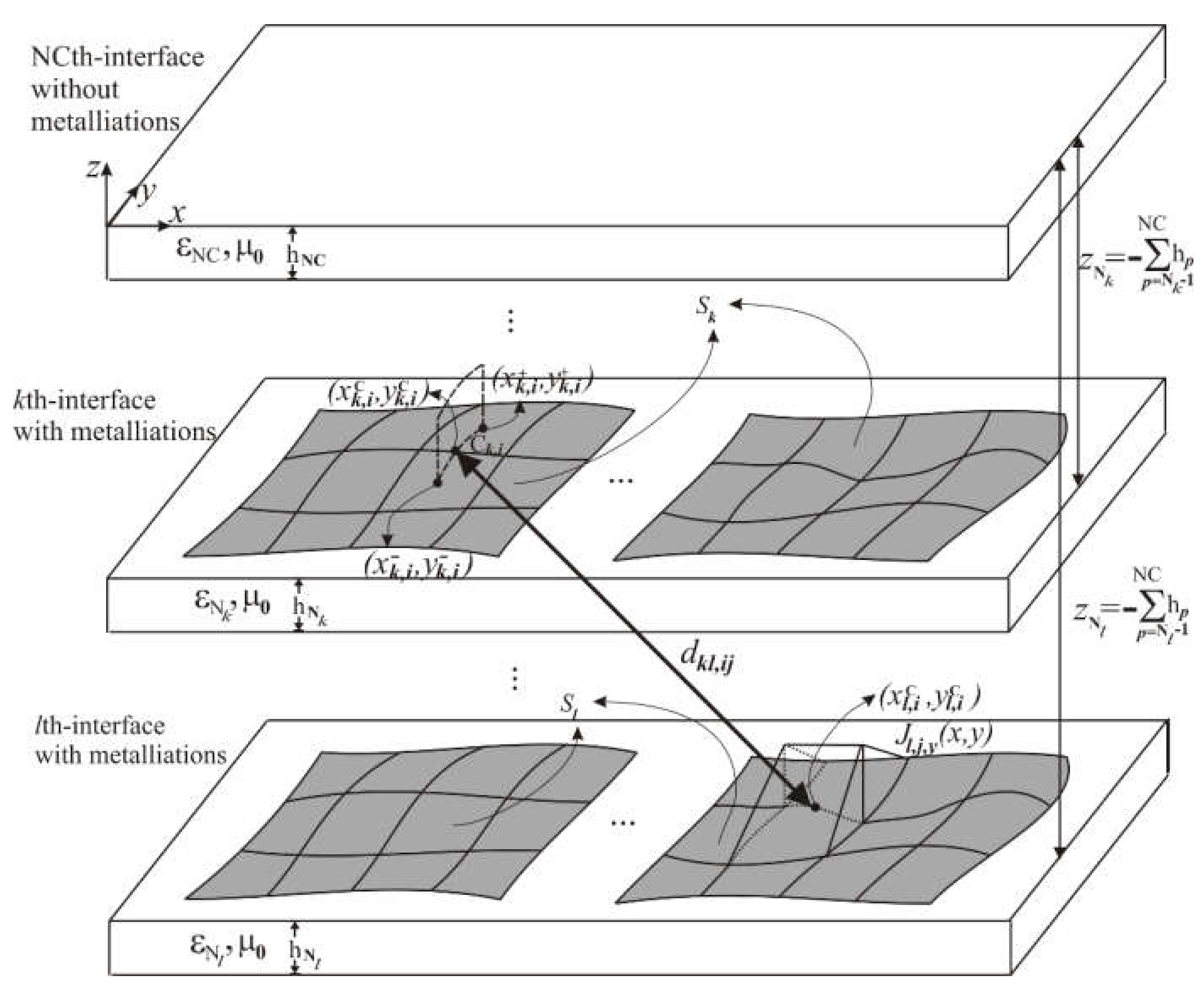
2. Description of the Problem

Let us consider a multilayer medium with NC dielectric layers of thickness d_p (p = 1, …, NC) and complex permittivity ε_p= ε₀ε_r,p(1 − jtanδ_p). The multilayer medium is upper limited by free space and lower limited by either free space or the ground plane. This multilayer medium hosts Q interfaces with metallized planar surfaces S_l (l = 1,…, Q) with negligible thickness and arbitrary geometry (see Figure 1). These metallized planar surfaces will be considered as PEC throughout. On each metallized surface S_l, surface current densities J_l(x,y) and charge densities σ_l(x,y) are induced by either fed voltage or incident electric field of arbitrary distribution. Both, current and charge densities are related by a known continuity equation. Since the surfaces S_l (l = 1,…, Q) are planar, the induced current densities J_l(x,y) have ‘x’ and ‘y’ components (i.e., there is not a z-component). These induced current densities satisfy the system of MPIEs from boundary conditions on PEC [7]. In order to solve the system of MPIEs, expansion in terms of known BFs (see (1)) with unknown coefficients (coefficients c_l,j shown in (1)) and the method of weighted residual are usual applied.

$$J_l(x,y)={\displaystyle \sum _{j=1}^{{\mathrm{N}}_{\mathrm{b},l}}{c}_{l,j,}{J}_{l,j}(x,y)};{\sigma }_l(x,y)={\displaystyle \sum _{j=1}^{{\mathrm{N}}_{\mathrm{b},l}}{c}_{l,j,}{\sigma }_{l,j}(x,y)};(l=1,\dots ,{\mathrm{Q};\mathrm{N}}_{\mathrm{b}}={\displaystyle \sum _{l=1}^{\mathrm{Q}}{\mathrm{N}}_{\mathrm{b},l}})$$

(1)

In this work the metallized planar surfaces were modeled by NURBS surfaces. The NURBS are discretized as piecewise Bezier patches [4]. Figure 1 shows metallized surfaces (grey color surfaces) with generic geometry, which are discretized as Bezier patches. So, subsectional generalized rooftop functions were used as BFs J_l,j(x,y) (j = 1,…, N_b,l; l = 1,…, Q) and razor-blade were used as weighting functions (WFs), both defined on two adjacent Bezier patches [4]. Figure 1 shows subsectional BFs of discretized metallized surfaces hosted in lth interface and a razor-blade function hosted in the kth-interface. The razor-blade joins the centers (x_k,i^+/−, y_k,i^+/−) of each adjacent Bezier patches by means the isoparametric curved lines C_k,i (i = 1,…, N_b,k, k = 1,…, Q) in the kth-interface. when the generalized rooftops were used as BFs and razor-blade were used as WFs, the resultant system of equations for the unknown coefficients c_l,j (j = 1,…, N_b,l; l = 1,…, Q) was obtained:

$${\displaystyle \sum _{l=1}^Q\left[V_{k,i,l}^{\mathrm{ind}}{(\mathrm{c}}_{1,1},\dots {,\mathrm{c}}_{{1,\mathrm{N}}_{\mathrm{b},l}})+V_{k,i,l}^{\mathrm{cap},+}{(\mathrm{c}}_{1,1},\dots {,\mathrm{c}}_{{1,\mathrm{N}}_{\mathrm{b},l}})-V_{k,i,l}^{\mathrm{cap},-}{(\mathrm{c}}_{1,1},\dots {,\mathrm{c}}_{{1,\mathrm{N}}_{\mathrm{b},l}})\right]}=V_{k,i}^{\mathrm{exc}};(i=1,\dots ,{\mathrm{N}}_{\mathrm{b},k};k=1,\dots ,\mathrm{Q})$$

(2)

where:

$$V_{k,i,l}^{\mathrm{ind}}=\mathrm{j}\omega {\displaystyle \underset{C_{i,k}}{\int }{f}_{k,l}^{\mathrm{ind}}(x,y)\cdot dr}$$

(3)

$$V_{k,i,l}^{\mathrm{cap},+/-}=f_{k,l}^{\mathrm{cap}}(x_{k,i}^{+/-},y_{k,i}^{+/-})$$

(4)

with:

$$f_{k,l}^{\mathrm{ind}}(x,y)={\displaystyle \underset{S_l}{\int }{\overline{G}}^{\mathrm{A}}(x-x\prime ,y-y\prime ,z=z_{N_k},z\prime =z_{N_l})J_l(x\prime ,y\prime )dx\prime dy\prime }$$

(5)

$$f_{k,l}^{\mathrm{cap}}(x,y)={\displaystyle \underset{S_l}{\int }{G}^{\mathsf{\Phi }}(x-x\prime ,y-y\prime ,z=z_{N_k},z\prime =z_{N_l}){\sigma }_l(x\prime ,y\prime )}dx\prime dy\prime$$

(6)

${\overline{G}}^{\mathrm{A}}$ is the dyadic Green’s function for the vector potential and G^Φ is the Green’s function for the scalar potential respectively of the multilayer medium of the Figure 1. In this work, formulation C of [28] was assumed. Since there is no z-component of surface current densities J_l(x’,y’), ${\overline{G}}^{\mathrm{A}}$ can be substituted by the Green’s function G^A_xx for the x-component of the vector potential throughout. In this work, two accurate techniques shown in [29,30] were used for computations of Green’s functions in both the near field region (i.e., when k₀ρ ≤ 10 with ρ = (x − x’)² + (y − y’)²]^1/2 and k₀ = 2π/λ being λ the vacuum wavelength) and far field regions (i.e., when k₀ρ > 10) respectively.

The coefficients V_k,i^exc of the system of linear equations given in (2) are either the feeding voltages defined on the ith-set of pair adjacent Bezier patches of the kth-interface or computed by the next line integral of the tangential component of excitation electric field E_t^exc(x,y,z = z_Nk) along the ith isoparametric curved line C_k,i on the kth-interface:

$$V_{k,i}^{\mathrm{exc}}={\displaystyle \underset{C_{k,i}}{\int }{E}_t^{\mathrm{exc}}(x,y,z=z_{{\mathrm{N}}_k})\cdot dr}$$

(7)

This excitation electric field is produced by the multilayer medium without metallizations when it is illuminated by incident electric field.

According to (1) and (2), a system with a total of N_b unknowns have to be solved. When large multilayer structures, which hosts resonant layouts have to be analyzed (for example, whole printed reflectarray antennas), hundreds of thousands of unknowns are expected. The direct solution of the resultant large system of equations produces drawbacks as large CPU consumption [8,9], large required CPU memory resources and ill-conditioned problems [10,11,12]. In order to avoid these drawbacks, an iterative solver are preferable where the unknowns c_l,j (j = 1,…, N_b,l; l = 1,…, Q) are iteratively computed to reduce a normalized error ξ, until threshold, ξ_th, is reached. In [23] the BICGSTAB method [31] was implemented as the iterative solver where the normalized error was defined as the following:

$$\xi =\frac{\left|V^{\mathrm{exc}}-V^{\mathrm{ind}}-V^{\mathrm{cap},+}+V^{\mathrm{cap},-}\right|}{\left|V^{\mathrm{exc}}\right|}$$

(8)

where:

$$\begin{array}{l}{V}^{\mathrm{exc}}=\left(V_{1,1}^{\mathrm{exc}},\dots ,V_{1,{\mathrm{N}}_{\mathrm{b},1}}^{\mathrm{exc}},\dots .,V_{\mathrm{Q},1}^{\mathrm{exc}},\dots ,V_{\mathrm{Q},{\mathrm{N}}_{\mathrm{b},\mathrm{Q}}}^{\mathrm{exc}}\right)\\ V^{\mathrm{ind}}=\left({\displaystyle \sum _{l=1}^Q{V}_{1,1,l}^{\mathrm{ind}}},\dots ,{\displaystyle \sum _{l=1}^Q{V}_{1,{\mathrm{N}}_{\mathrm{b},1},l}^{\mathrm{ind}}},\dots .,{\displaystyle \sum _{l=1}^Q{V}_{Q,1,l}^{\mathrm{ind}}},\dots ,{\displaystyle \sum _{l=1}^Q{V}_{Q,{\mathrm{N}}_{\mathrm{b},\mathrm{Q}},l}^{\mathrm{ind}}}\right)\\ V^{\mathrm{cap},+/-}=\left({\displaystyle \sum _{l=1}^Q{V}_{1,1,l}^{\mathrm{cap},+/-}},\dots ,{\displaystyle \sum _{l=1}^Q{V}_{1,{\mathrm{N}}_{\mathrm{b},1},l}^{\mathrm{cap},+/-}},\dots .,{\displaystyle \sum _{l=1}^Q{V}_{Q,1,l}^{\mathrm{cap},+/-}},\dots ,{\displaystyle \sum _{l=1}^Q{V}_{Q,{\mathrm{N}}_{\mathrm{b},\mathrm{Q}},l}^{\mathrm{cap},+/-}}\right)\end{array}$$

(9)

Note that V^ind, V^cap,+, and V^cap,− have to be computed in each iteration in the iterative process for fixed values of c_l,j (j = 1,…, N_b,l; l = 1,…, Q). If this computation is carried out by direct computation of (3) and (4) using (5) and (6), the CPU time consumption can be prohibitive due to slow continuous convolutions between Green’s functions and currents or charges densities shown in (5) and (6). In [23], a very efficient technique was proposed for fast computation of V^ind, V^cap,+, and V^cap,− using pulse expansion of BFs and the EPP approach. This pulse expansion is carried out by means of approximations of the BFs in terms of constants pulses in a very dense regular mesh [32]:

$$J_{l,j}(x\prime ,y\prime )\approx {\displaystyle \sum _{m\prime =0}^{2N_x+1}{\displaystyle \sum _{n\prime =0}^{2N_y+1}{J}_{l,j}(x_{m\prime },y_{n\prime })P(x\prime -x_{m\prime },y\prime -y_{n\prime })}}$$

(10)

$${\sigma }_{l,j}(x\prime ,y\prime )\approx {\displaystyle \sum _{m\prime =0}^{2N_x+1}{\displaystyle \sum _{n\prime =0}^{2N_y+1}{\sigma }_{l,j}(x_{m\prime },y_{n\prime })P(x\prime -x_{m\prime },y\prime -y_{n\prime })}}$$

(11)

where x_m’ = x₀ + m’Δx, y_n’ = y₀ + n’Δy and Δx = 2L_x/(2N_x + 1), and Δy = 2L_y/(2N_y + 1) with (2L_x) × (2L_y) the minimum rectangle that hosts the whole multilayer structure with maximum dimensions L_x × L_y. This minimum rectangle ensures that aliasing is avoided [14,23]. The function P(x’ − x_m’, y’ − y_n’) is one when x_m’ − Δx/2 < x<x_m’ + Δx/2 and y_n’ − Δy/2 < y < y_n’ + Δy/2 and zero elsewhere. So, constant pulses on x_m’ − Δx/2 < x < x_m’ + Δx/2 and y_n’ − Δy/2 < y< y_n’ + Δy/2 are defined with values of BFs on regular mesh points (x_m’, y_n’). Figure 2 shows the regular mesh points (x_m’, y_n’) of the lth interface for an example of two ellipse halves of layout geometry.

The pulse expansion of BFs given in (10) and (11) leads discrete cyclic convolutions instead of the continuous convolutions shown in (5) and (6) when the functions f_k,l^ind(x,y) and f_k,l^cap(x,y) are evaluated in the samples x_m = x₀ + mΔx and y_n = y₀ + nΔy. These discrete cyclic convolutions are shown as the following [32]:

$$f_{k,l,x/y}^{\mathrm{ind}}(x_m,y_n)={\displaystyle \sum _{m\prime =0}^{2N_x+1}{\displaystyle \sum _{n\prime =0}^{2N_y+1}{J}_{l,x/y}^{\mathrm{d}}[m\prime ,n\prime ]G_{k,l}^{\mathrm{d},\mathrm{A}}[m-m\prime ,n-n\prime ]}}$$

(12)

$$f_{k,l}^{\mathrm{cap}}(x_m,y_n)={\displaystyle \sum _{m\prime =0}^{2N_x+1}{\displaystyle \sum _{n\prime =0}^{2N_y+1}{\sigma }_l^{\mathrm{d}}[m\prime ,n\prime ]G_{k,l}^{\mathrm{d},\mathsf{\Phi }}[m-m\prime ,n-n\prime ]}}$$

(13)

where the discrete functions J^d_l,x/y[m’,n’], σ^d_l[m’,n’], G_k,l^d,A[m − m’, n − n’], and G_k,l^d,Φ[m − m’, n − n’] are shown below [23] when 0 ≤ m’ ≤ N_x and 0 ≤ n’ ≤ N_y:

$$J_{l,x/y}^{\mathrm{d}}[m\prime ,n\prime ]={\displaystyle \sum _{j=1}^{{\mathrm{N}}_{\mathrm{b},l}}{c}_{l,j}{J}_{l,j,x/y}(x_{m\prime },y_{n\prime })}$$

(14)

$${\sigma }_l^{\mathrm{d}}[m\prime ,n\prime ]={\displaystyle \sum _{j=1}^{{\mathrm{N}}_{\mathrm{b},l}}{c}_{l,j}{\sigma }_{l,j}(x_{m\prime },y_{n\prime })}$$

(15)

$$G_{k,l}^{\mathrm{d},\mathrm{A}}[m-m\prime ,n-n\prime ]={\displaystyle \underset{x_{m\prime }-\frac{\Delta x}{2}}{\overset{x_{m\prime }+\frac{\Delta x}{2}}{\int }}{\displaystyle \underset{y_{n\prime }-\frac{\Delta y}{2}}{\overset{y_{n\prime }+\frac{\Delta y}{2}}{\int }}{G}_{xx}^{\mathrm{A}}(x_m-x\prime ,y_n-y\prime ,z=z_{{\mathrm{N}}_k},z\prime =z_{{\mathrm{N}}_l})dx\prime dy\prime }}$$

(16)

$$G_{k,l}^{\mathrm{d},\mathsf{\Phi }}[m-m\prime ,n-n\prime ]={\displaystyle \underset{x_{m\prime }-\frac{\Delta x}{2}}{\overset{x_{m\prime }+\frac{\Delta x}{2}}{\int }}{\displaystyle \underset{y_{n\prime }-\frac{\Delta y}{2}}{\overset{y_{n\prime }+\frac{\Delta y}{2}}{\int }}{G}^{\mathsf{\Phi }}(x_m-x\prime ,y_n-y\prime ,z=z_{{\mathrm{N}}_k},z\prime =z_{{\mathrm{N}}_l})dx\prime dy\prime }}$$

(17)

These discrete functions have (2N_x + 2) × (2N_y + 2) elements. Zero padding of the discrete functions J^d_l,x/y[m’,n’] and σ^d_l[m’,n’] is carried out when m’ > N_x, n’ > N_y. In order to avoid unnecessary computations by means of (16) and (17), the following conditions are also imposed on G_k,l^d,A[m − m’, n − n’] and G_k,l^d,Φ[m − m’, n − n’] when m’ > N_x, n’ > N_y.

$$G_{k,l}^{\mathrm{d},\mathrm{A}/\mathsf{\Phi }}[m-m\prime ,n-n\prime ]=\left\{\begin{array}{l}{G}_{k,l}^{\mathrm{d},\mathrm{A}/\mathsf{\Phi }}[2N_x+2-(m-m\prime ),n-n\prime ]\mathrm{if}{N}_x<m-m\prime ;n-n\prime \le N_y\\ G_{k,l}^{\mathrm{d},\mathrm{A}/\mathsf{\Phi }}[m-m\prime ,2N_y+2-(n-n\prime )]\mathrm{if}{N}_y<n-n\prime ;m-m\prime \le N_x\\ G_{k,l}^{\mathrm{d},\mathrm{A}/\mathsf{\Phi }}[2N_x+2-(m-m\prime ),2N_y+2-(n-n\prime )]\mathrm{if}{N}_x<m-m\prime ;N_y<n-n\prime \end{array}\right.$$

(18)

All these discrete functions lead the cyclic discrete convolutions given in (12) and (13) instead of the continuous convolutions shown in (5) and (6). These discrete cyclic convolutions can be efficiently computed by means of FFT-accelerated matrix–vector multiplication [24,32]. Once the discrete cyclic convolutions are available, the functions f_k,l^ind(x,y) and f_k,l^cap(x,y) defined in (5) and (6), which are required in (3) and (4), are approximated in the observation points (x,y) from the samples f_k,l^ind(x_m,y_n) and f_k,l^cap(x_m,y_n) on the dense regular mesh using conventional bilinear interpolation [33].

Although these approaches lead to fast computation of normalized error ξ of the iterative process, any preconditioner was not included in [23]. The main advantage of the uses of a preconditioner in the iterative method is that it leads a transformation of the linear system of equations with more favorable spectral properties of the original system of equations. These favorable spectral properties ensure a significant increment of the rate of convergence of the iterative method [23]. These favorable spectral properties are guaranteed if the resultant matrix obtained from standard matrix product between the coefficient matrix of the linear system and preconditioner matrix is as close to the identity matrix as possible [25]. A very popular preconditioner is a sparse approximate inverse (SAI) preconditioner [25,26,27]. This SAI preconditioner is computed as a matrix that minimizes the Frobenius’ norm of the difference between identity matrix and standard matrix product between the SAI matrix and coefficient matrix of the linear system of equations given in (2) [26,27]. This minimization can be efficiently computed by solving independent linear least square (LLS) systems that generate the rows of the preconditioner [27]. However, the system of equations given in (2) provides a coefficient matrix of a very large size and its computation involves very large CPU time consumption. In order to save CPU time the SAI preconditioner is often generated from a reduced coefficient matrix, which only considers the near field part of the coefficient matrix. This near field part includes the strongest interactions between BFs and WFs [27]. These interactions between BFs and WFs are usually considered in the near field part when the distances between BFs and WFs are less than one quarter of the wavelength under analysis. So, the elements of the reduced coefficient matrix are defined as the following:

$$Z_{kl,ij}^R=\left\{\begin{array}{ll}0& \mathrm{if}{d}_{kl,ij}>\lambda /4\\ Z_{kl,ij}^{\mathrm{ind}}+Z_{kl,ij}^{\mathrm{cap},+}-Z_{kl,ij}^{\mathrm{cap},-}& \mathrm{if}{d}_{kl,ij}\le \lambda /4\end{array}\right.$$

(19)

where:

$$Z_{kl,ij}^{\mathrm{ind}}=\mathrm{j}\omega {\displaystyle \underset{C_{i,k}}{\int }{f}_{k,l,j}^{\mathrm{ind}}(x,y)\cdot dr}$$

(20)

$$Z_{kl,ij}^{\mathrm{cap},+/-}=f_{k,l,j}^{\mathrm{cap}}(x_{k,i}^{+/-},y_{k,i}^{+/-})$$

(21)

$$f_{k,l,j}^{\mathrm{ind}}(x,y)={\displaystyle \underset{S_{l,j}}{\int }{\overline{G}}^{\mathrm{A}}(x-x\prime ,y-y\prime ,z=z_{N_k},z\prime =z_{N_l})J_{l,j}(x\prime ,y\prime )dx\prime dy\prime }$$

(22)

$$f_{k,l,j}^{\mathrm{cap}}(x,y)={\displaystyle \underset{S_{l,j}}{\int }{G}^{\mathsf{\Phi }}(x-x\prime ,y-y\prime ,z=z_{N_k},z\prime =z_{N_l}){\sigma }_{l,j}(x\prime ,y\prime )}dx\prime dy\prime$$

(23)

where d_kl,ij are the distance between the centers of BFs hosted in the lth interface and the centers of WFs hosted in the kth interface (see Figure 1), and S_l,j is the surface of the pair of adjacent Bézier patches where jth-BF is defined in the lth interface. Therefore, once the reduced coefficient matrix is available, the SAI preconditioner is computed as a matrix, which minimizes the following Frobenius’ norm:

$$\min {‖I-M\cdot Z^R‖}_F^2={\displaystyle \sum _{s=1}^{{\mathrm{N}}_{\mathrm{b}}}\min {‖e_s-m_s\cdot Z^R‖}_F^2}$$

(24)

where I is the identity matrix of N_b × N_b size, M is the SAI preconditioner matrix, e_s is the sth-row of the identity matrix, and m_s is the sth-row of the preconditioner matrix M. In [27] a sophisticated compartmentalization of the computational space in terms of regions is shown. The description of this compartmentalization is out of the scope of this section and we recommend [27] for a detailed description. So, once the SAI preconditioner matrix M is available, the BICGSTAB method [31] can be implemented for iteratively solving of a modified system of equations with a higher rate of convergence than the original system of the equation shown in (2):

$$M\cdot {\left[V^{\mathrm{ind}}+V^{\mathrm{cap},+}-V^{\mathrm{cap},-}\right]}^T=M\cdot {\left[V^{\mathrm{exc}}\right]}^T$$

(25)

where superscript T denotes the transposed matrix. Note that the inductive and capacitive contributions given in (20) and (21) should be computed when the distances d_kl,ij are less than one quarter of the wavelength. In this case continuous convolutions between Green’s functions and BFs shown in (22) and (23) should be computed instead of continuous convolutions between Green’s functions and surface current and charge densities shown in (5) and (6) (note that the functions f_k,l,j^ind(x,y) and f_k,l,j^cap(x,y) stand for the convolution between Green’s functions and a BF hosted in the lth-interface while that, the functions f_k,l^ind(x,y) and f_k,l^cap(x,y) stand for the convolution between Green’s functions and current and charge densities hosted in the lth-interface). If the computations are directly carried out by means of (22) and (23), large CPU time is consumed. In order to accelerate the computation of (22) and (23), again pulse expansion of BFs and EPP can be carried out to lead discrete cyclic convolutions instead of the continuous convolution [32]. Since matrix elements of Z^R_kl,ij are only computed when d_kl,ij < λ/4 the domain of required EPP for the efficient computation of (22) and (23) is only one half of the wavelength (two times one quarter of wavelength) in order to avoid aliasing. This domain is much less than that required whole size L_x × L_y of the large multilayer medium under study. So, similar pulse expansion shown in (10) and (11) is carried out but on a new regular mesh samples x_m’R and y_n’R:

$$\left\{\begin{array}{c}{x}_{m{\prime }_R}=x_{0,l,j}+m{\prime }_R\Delta x_R-\lambda /4\mathrm{if}0\le m{\prime }_R\le 2N_x^R+1\\ y_{n{\prime }_R}=y_{0,l,j}+n{\prime }_R\Delta y_R-\lambda /4\mathrm{if}0\le n{\prime }_R\le 2N_y^R+1\end{array}\right.$$

(26)

where Δx_R = λ/[2(2N^R_x + 2)] and Δy_R = λ/[2(2N^R_x + 2)] being x_0,l,j and y_0,l,j the minimum values of the Cartesian coordinates of the pair adjacent Bezier patches where the jth BF is defined in the lth-interface with metallizations. In this way, the following discrete functions of (2N^R_x + 2) × (2N^R_y + 2) elements for the BFs hosted in the lth-interface with metallizations were used when 0 ≤ m’_R ≤ N^R_x and 0 ≤ n’_R ≤ N^R_y:

$$J_{l,j,x/y}^{\mathrm{d}}[m{\prime }_R,n{\prime }_R]=J_{l,j,x/y}(x_{m{\prime }_R},y_{n{\prime }_R})$$

(27)

$${\sigma }_{l,j}^{\mathrm{d}}[m{\prime }_R,n{\prime }_R]={\sigma }_{l,j}(x_{m{\prime }_R},y_{n{\prime }_R})$$

(28)

Again, zero padding of the discrete functions is carried out when m’_R > N^R_x and n’_R > N^R_y. Similar periodic discrete functions for the multilayer Green’s functions defined in (16), (17), and (18) were used but with N^R_x and N^R_y instead of N_x and N_y, Δx_R, and Δy_R instead of Δx and Δy, and x_m’R and y_n’R instead of x_m and y_n. These new discrete functions lead the following discrete cyclic convolutions when the functions f_k,l,j^ind(x,y) and f_k,l,j^cap(x,y) are evaluated in the samples x_m’R and y_n’R:

$$f_{k,l,j,x/y}^{\mathrm{ind}}(x_{m_R},y_{n_R})={\displaystyle \sum _{m{\prime }_R=0}^{2N_x^R+1}{\displaystyle \sum _{n{\prime }_R=0}^{2N_y^R+1}{J}_{l,j,x/y}^{\mathrm{d}}[m{\prime }_R,n{\prime }_R]G_{k,l}^{\mathrm{d},\mathrm{A}}[m_R-m{\prime }_R,n_R-n{\prime }_R]}}$$

(29)

$$f_{k,l,j}^{\mathrm{cap}}(x_{m_R},y_{n_R})={\displaystyle \sum _{m{\prime }_R=0}^{2N_x^R+1}{\displaystyle \sum _{n{\prime }_R=0}^{2N_x^R+1}{\sigma }_{l,j}^{\mathrm{d}}[m{\prime }_R,n{\prime }_R]G_{k,l}^{\mathrm{d},\mathsf{\Phi }}[m_R-m{\prime }_R,n_R-n{\prime }_R]}}$$

(30)

Again, these discrete cyclic convolutions can be efficiently computed by means of FFT-accelerated matrix–vector multiplication [24,32]. Once the discrete cyclic convolutions are available, the functions f_k,l,j^ind(x,y) and f_k,l,j^cap(x,y) defined in (22) and (23), which are required in (20) and (21), are approximated in the observation points (x,y) from the samples f_k,l,j^ind(x_m’R,y_n’R) and f_k,l,j^cap(x_m’R,y_n’R) on regular mesh using conventional bilinear interpolation [33].

Note that the size of the domain of the samples x_m’R and y_n’R is (λ/2) × (λ/2) while the size domain of the samples x_m’ and y_n’ is (2L_x) × (2L_y), which is much larger than (λ/2) × (λ/2) for large whole multilayer structures. This fact leads to values of N^R_x and N^R_y to be much less than N_x and N_y. So, these small values of N^R_x and N^R_y lead to very fast computation of the reduced coefficient matrix given in (19) to generate a SAI preconditioner as it is shown in the Section 3.

3. Numerical Results

In this section we will show results of three analyses of whole printed reflectarray antennas: (1) focused beam reflectarray made of two sets of four parallel dipoles with small rotations, (2) reflectarray made of two orthogonal sets of four parallel dipoles to generate South-American coverage, and (3) dual band circular polarized focused beam reflectarray made of dual concentric split rings.

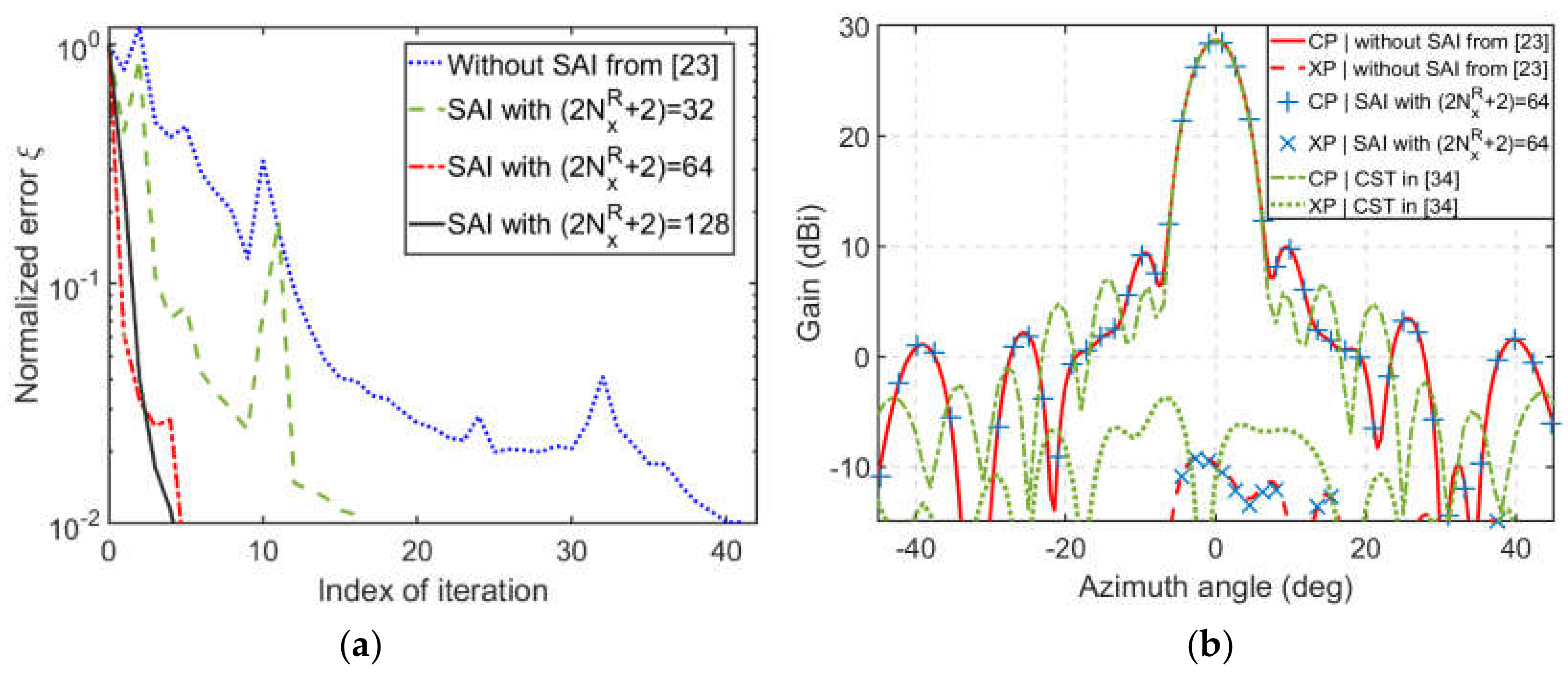
3.1. Focused Beam Reflectarray Made of Two Sets of Four Parallel Dipoles with Small Rotations

In [34] a 24 cm square focused beam reflectarray was designed at 11.95 GHz under local periodicity assumption and analyzed with CST commercial software. The square reflectarray was made of two orthogonal sets of parallel dipoles. Each set of parallel dipoles is displaced half a period from each other with small rotations in order to reduce cross-polar radiation (see Figure 2 in [34] for details). The cell size of each reflectarray element is 12 × 12 mm² for each set of parallel dipoles. So, the reflectarray consists of a 20 × 20 square grid (the electrical size of the reflectarray is 9.6λ × 9.6λ at 11.95 GHz). The reflectarray was designed to focus the main beam at 11.95 GHz for the angular spherical coordinates θ_beam = 16.9° φ_beam = 0° with respect to the coordinate system located at the center of reflectarray. An upper dielectric layer of Diclad 880 (ε_r,2 = 2.17, tanδ₂ = 0.0009) of 1.5 mm thick hosts the printed dipoles and a bottom dielectric layer of Arlon AD255C layer (ε_r,1 = 2.55, tanδ₁= 0.0014) 2.363 mm thick was used as a separator with the ground plane. In [23] this reflectarray was analyzed by the iterative method using pulse expansion and EPP approaches with (2N_x + 2) × (2N_y + 2) = 4096 × 4096 for the computation of normalized error ξ. In this analysis a model cos¹⁰(θ) of the feeder located at (x_F, y_F, z_F)= (−85.3, 0, 281) (mm) and 23,548 generalized rooftops in the approximation of the surface density currents (i.e., the number of unknowns is N_b = 23,548) was considered. In this work the reflectarray was analyzed with a SAI preconditioner computed from the reduced coefficient matrix given in (19) and the proposed discretization given in (26) for the discrete functions of (27) and (28), and discrete cyclic convolution given in (29) and (30). Different values of the (2N^R_x + 2) × (2N^R_y + 2) elements of the discrete functions were considered in the computation of reduced coefficient matrix: (2N^R_x + 2) × (2N^R_y + 2) = 32 × 32, (2N^R_x + 2) × (2N^R_y + 2) = 64 × 64, and (2N^R_x + 2) × (2N^R_y + 2) = 128 × 128. Note that these values are much less than (2N_x + 2) × (2N_y + 2) = 4096 × 4096. A total of 528,052 elements from the N_b × N_b = 23,548 × 23,548 elements of the reduced coefficient matrix satisfy the condition d_kl,ij < λ/4.

Table 1. A total of 528,052 elements of the reduced matrix satisfy the condition d_kl,ij < λ/4.

2Nx + 2	CPU Time (s)
32	19
64	47
128	278

shows the CPU time consumption in the computation of the reduced coefficient matrix given in (19).

Once the reduced coefficient matrix is available, the SAI preconditioner matrix M is computed according to the minimization problems shown in (24). When this SAI preconditioner matrix M is known, the BICGSTAB method [31] can be implemented as the iterative solver for solving a modified system of equations shown in (25). Figure 3a shows a comparison between the normalized error ξ with respect to of the index of iteration when the SAI preconditioner is not used and when the SAI preconditioner is computed using the different values of (2N^R_x + 2) × (2N^R_y + 2). We would like to point out that 90 s are required per iteration. According to Figure 3a, CPU time consumptions to reach the threshold ξ_th = 0.01 were 61.5 min when SAI was not used (i.e., 41 iterations were required), 25.5 min when SAI was used with (2N^R_x + 2) × (2N^R_y + 2) = 32 × 32 (i.e., 17 iterations were required), and 7.5 min when SAI was used with (2N^R_x + 2) × (2N^R_y + 2) = 64 × 64 and (2N^R_x + 2) × (2N^R_y + 2) = 128 × 128 (i.e., 5 iterations were required). All these results were obtained in a laptop computer with an Intel processor Core i7-6700HQ, 2.6 GHz of clock frequency with 32 GBytes of RAM memory. Note that when (2N^R_x + 2) × (2N^R_y + 2) = 64 × 64 a maximum reduction of required iterations was produced to reach the threshold ξ_th = 0.01 with respect to those required iterations when SAI preconditioner was not used (i.e., the iterative method with SAI preconditioner was 8.2 times faster than the iterative method without preconditioner). Moreover, when (2N^R_x + 2) × (2N^R_y + 2) = 64 × 64 the CPU time consumption for the computation of the reduced coefficient matrix was 47 s (see Table 1). This CPU time consumption was not significant with respect to the 7.5 min consumed by the iterative process to reach the threshold ξ_th = 0.01 (less than 11% of the full time). Figure 3b shows numerical copolar and cross-polar radiation patterns in the azimuth plane for X polarization at 11.95 GHz. These results were compared with results obtained in [23] when a SAI preconditioner was not used and with results obtained by full-wave simulation of the whole antenna with CST shown in Figure 5b of [34]. We can see that identical results were obtained by means SAI preconditioner with respect to those shown in [23] when SAI preconditioner was not used. We can see that acceptable agreements were found with results provided by CST in [34]. However, the cross-polar radiation levels obtained by CST were higher than the cross-polar radiation obtained by the proposed method. As it is explained in [23], this is expected since the full-wave model of the feed horn was carried out by CST (we remind that a cos¹⁰(θ) model of the feeder was used in our analysis). According with [34], the analysis of the whole antenna provided by CST took 8 h in a computer with 2 Intel Xeon Processors (6 cores per processor), 2.1 GHz of clock frequency, and 128 GBytes of RAM memory. Note that our simulations with a SAI preconditioner is roughly 64 times faster than the CST simulations using a laptop with lower performances than the computer used in [34].

3.2. Reflectarray Made of Two Orthogonal Sets of Four Parallel Dipoles to Generate South American Coverage

A reflectarray of 1.1 m of diameter designed to generate a South American coverage at 11.95 GHz (i.e., the electrical size of the reflectarray was roughly 44λ × 44) was analyzed in this subsection. This reflectarray was designed in [35] with the stringent coverage requirements of minimum gain given in [36,37]. The reflectarray was made of the same reflectarray element of the previous subsection (again Diclad 880 and Arlon AD255C layers of 1.5 and 2.363 mm thick were used) but, in this case the cell size of each reflectarray element was 10 × 12 mm² for each set of parallel dipoles. Unlike the previous case the dipoles were not rotated. So, the reflectarray consists of 7772 elements arranged in a 110 × 90 rectangular grid (see Figure 4a,b). In [35] the reflectarray is fed by a corrugated circular horn with phase center located at the point of coordinates (x_F, y_F, z_F) = (−366, 0, 1451) (mm) with respect to the system coordinate system located at the center of the reflectarray. In our analysis we considered the cos²⁶(θ) model of the feeder. This reflectarray was analyzed by an iterative method using pulse expansion and EPP approaches with (2N_x + 2) × (2N_y + 2) = 16,384 × 16,384 for the computation of normalized error ξ. Note that these values were much higher than those used in the previous subsection. This is due to the large electrical size of the reflectarray. Since the vacuum wavelength was equal to that used in the previous subsection, values of (2N^R_x + 2) × (2N^R_y + 2) = 64 × 64 were considered in the computation of reduced coefficient matrix. In this case 493,190 generalized rooftops were considered in the approximation of the surface currents (i.e., the number of unknowns was N_b = 493,190). A total of 14,299,768 elements from the N_b × N_b = 493,190 × 493,190 elements of the reduced coefficient matrix satisfied the condition d_kl,ij < λ/4 The CPU time consumption in the computation of the reduced coefficient matrix was roughly 39 min. This CPU time consumption was much larger than shown in Table 1 when 2N^R_x + 2 = 64. This fact is because the number of elements that satisfy the condition d_kl,ij < λ/4 was roughly 27 times larger than those obtained in the previous subsection. Analysis of the reflectarray antenna was carried out by the iterative method when the SAI preconditioner was not used and when the SAI preconditioner was computed using the values of (2N^R_x + 2) × (2N^R_y + 2) = 64 × 64. All simulations were carried out in a computer of high performances with processor Intel Xeon Silver 4110 2.10 GHz of clock frequency with 192 GBytes of RAM memory. We would like to point out that 19 iterations were required to reach the threshold ξ_th = 0.01 when the SAI preconditioner was used but 87 iterations were required when the SAI preconditioner was not used. In these analyses 6.5 min were required per iteration. So, a total CPU time consumption of 2.7 h (including the computation of the reduced coefficient matrix) were required to reach the threshold when the SAI preconditioner was used while a total CPU time consumption of 9.4 h were required when the SAI preconditioner was not used. Figure 4c shows contour lines of radiation patterns for X-polarization at 11.95 GHz obtained by the iterative method with the SAI preconditioner. Identical results were obtained by the iterative method when the SAI preconditioner was not used (not shown). Comparison with numerical results given in [35] and templates for South American coverage with requirements of minimum gains are also shown. We can see that the requirements of minimum gains were roughly satisfied. There were some discrepancies between contour lines provided by the iterative method and results given in [35]. The results given in [35] were obtained under local periodicity assumption while our results were obtained by a full-wave analysis of the structure. So, these discrepancies were expected.

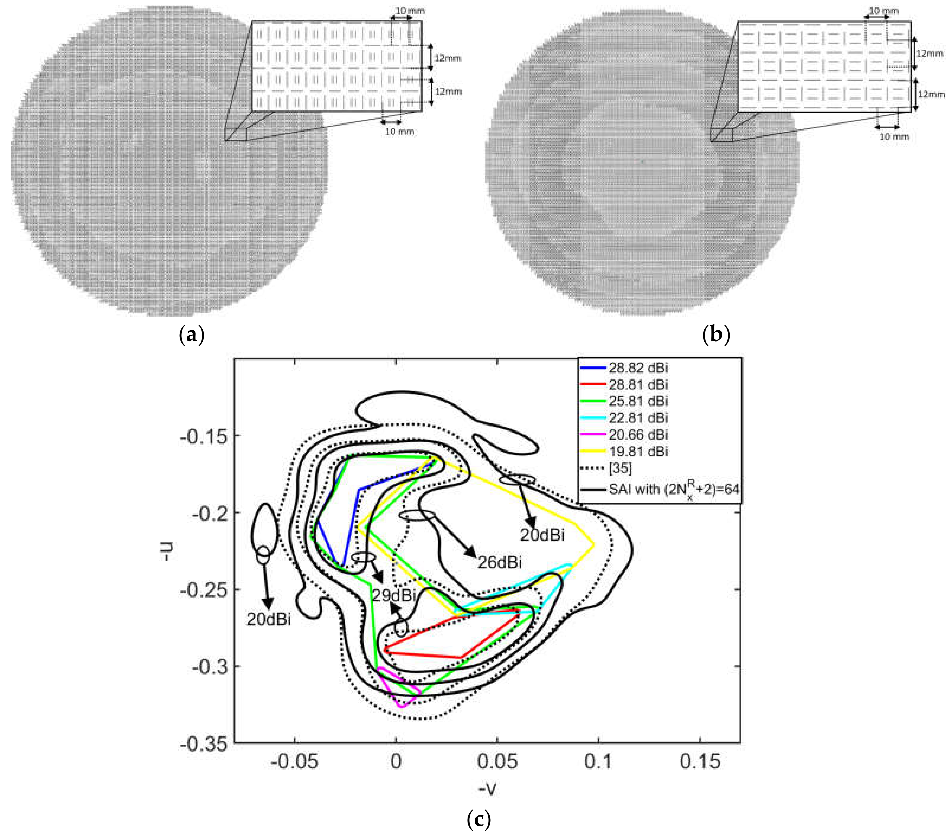
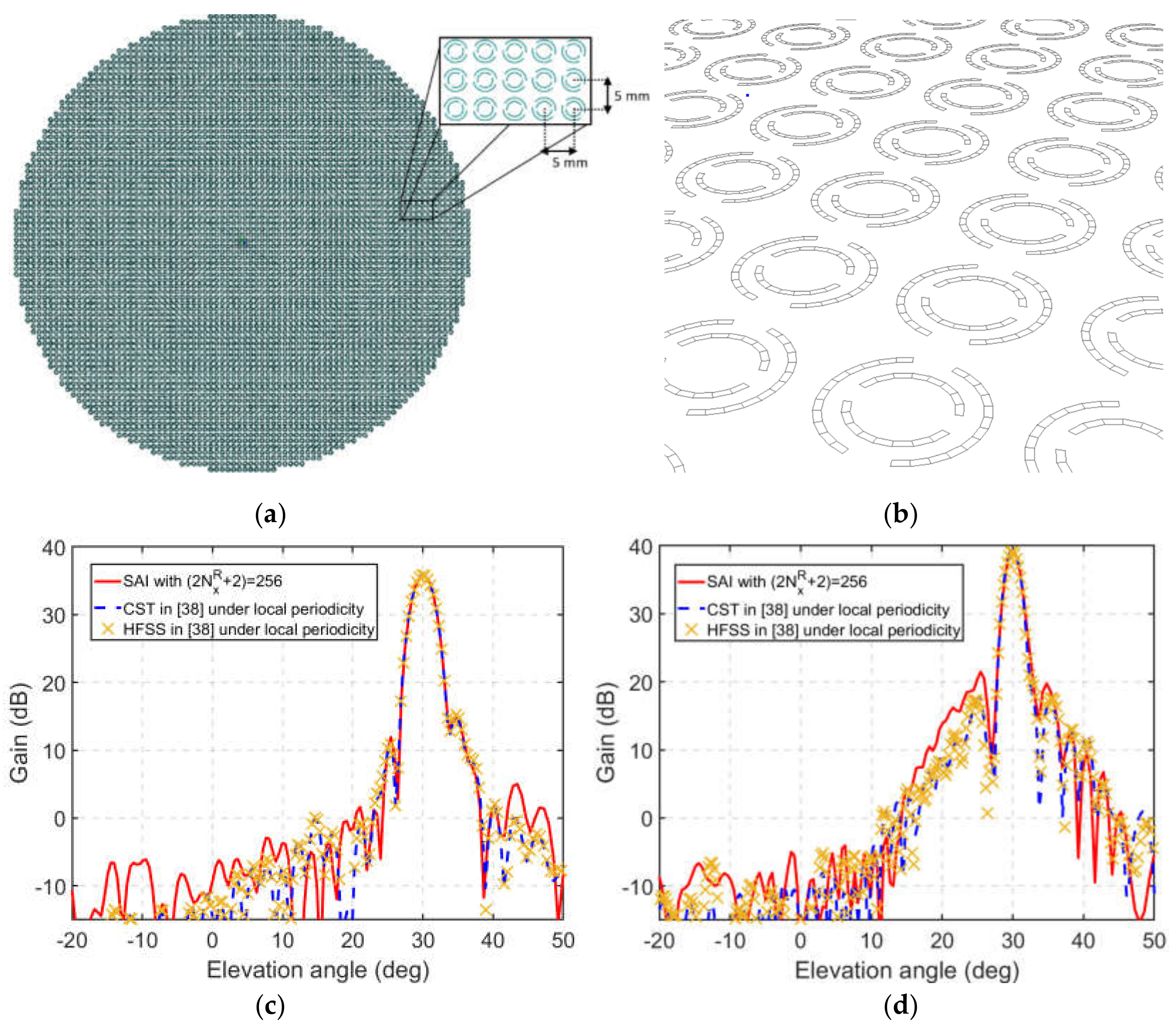
3.3. Dual Band Circular Polarized Focused Beam Reflectarray Made of Dual Concentric Split Rings

In [38] a dual band circular polarized focused beam reflectarray made of dual concentric split rings was designed using the procedure given in [39] following the variable rotation technique (VRT). The VRT requires that the reflection coefficients of the two orthogonal linear components of the impinging wave electric field are of equal magnitude and 180° out of phase in order to keep the sense of CP after reflection [40,41]. The designed reflectarray was made to focus the main beam in the direction given by angular spherical coordinates θ_beam = 30° φ_beam = 0° with respect to the coordinate system located at the center of reflectarray at 19.95 GHz for left-handed circular polarization (LHCP) and at 29.75 GHz for right-handed circular polarization (RHCP). In this way, the outer split-rings work at 19.95 GHz (i.e., the arc lengths and rotations of outer split-rings were adjusted at 19.95 GHz) while the inner split-rings work at 29.75 GHz (i.e., the arc lengths and rotations of inner split-rings were adjusted at 29.75 GHz). The adjustments of arc lengths and rotations of split rings were carried out with a fixed outer radius of 2.05 mm for outer split-rings and 1.40 mm for inner split rings. The width of the split rings was also fixed at 0.2 mm. These fixed dimensions provide a 0.45 mm of separation between outer and inner split rings. So, strong couplings between outer and inner split rings were expected. The designed antenna was circular and consists of 5024 elements arranged in 80 × 80 grid with cell size 5 mm × 5 mm (see Figure 5a for layout). Note that the electrical size of the reflectarray was roughly 27λ × 27λ at 19.95 GHz and 40λ × 40λ at 29.75 GHz. The split rings were printed on single layer Roger Duroid 5880 (ε_r,1 = 2.2, tanδ₁ = 0.0009) 0.787 mm thick, which was bottom limited by a ground plane. Since the use of Bézier patches of NURBS surfaces for the discretization of the geometry is an important feature of the proposed technique, the meshing of dual concentric split-rings is shown in Figure 5b. It would be interesting to see how NURBS were used in the discretization of the examples The reflectarray was illuminated by a corrugated circular feed horn with its phase center located at the coordinates x = −150 mm, y = 0 mm, and z = 259.8 mm with respect to a coordinate system with the origin at the center of the reflectarray. The horn was assumed to radiate LHCP waves at 19.95 GHz and RHCP waves at 29.75 GHz. The radiation pattern of the horn was modeled as a function cos⁷(θ), which provides an illumination level at the reflectarray edges 12 dB below the maximum. This reflectarray was analyzed by the iterative method using pulse expansion and EPP approaches with (2N_x + 2) × (2N_y + 2) = 8192 × 8192 for the computation of normalized error ξ. In this case values of (2N^R_x + 2) × (2N^R_y + 2) = 256 × 256 were considered at each frequency for the computation of reduced coefficient matrix. In the approximation of the surface density currents, 180,886 generalized rooftops were considered. In the case of the analysis at 19.95 GHz a total of 5,221,352 elements from the N_b × N_b = 180,886 × 180,886 elements of the reduced coefficient matrix satisfied the condition d_kl,ij < λ/4 while a total of 2,536,966 elements satisfied the same condition at 29.75 GHz. The CPU time consumption in the computation of the reduced coefficient matrix was roughly 24.3 min at 19.95 GHz and 17.8 min at 29.75 GHz. The analysis of the reflectarray antenna at both frequencies were carried out by the iterative method when SAI preconditioner was not used and when the SAI preconditioner was computed using the values of (2N^R_x + 2) × (2N^R_y + 2) = 256 × 256. These all simulations were carried out in a laptop computer with processor Intel Core i7-6700HQ, 2.6 GHz of clock frequency with 32 GBytes of RAM memory. We would like to point out that when the analysis was carried out at 19.95 GHz, four iterations were only required to reach the threshold ξ_th = 0.01 when the SAI preconditioner was used while 170 iterations were required when the SAI preconditioner was not used. In the case of analysis at 29.75 GHz, 10 iterations were only required when the SAI preconditioner was used while 415 iterations were required when the SAI preconditioner was not used. These large amounts of 170 and 415 iterations were attributed the strong couplings between outer and inner split rings. Since strong coupling between outer and inner split rings was expected, high sensitivity of the surface current densities was also expected. This sensitivity obstructed the reduction of normalized error ξ by the iterative process. Moreover, the outer split rings produced a stronger effect on the electrical behavior of inner split rings at 29.75 GHz than the effect produced by the inner split ring on the electrical behavior of outer split rings at 19.95 GHz. So, it is expected that more iterations were required at 29.75 GHz than those required at 19.95 GHz. In these analyses 2.15 min were required per iteration at both frequencies 19.95 and 29.75 GHz. So, a total CPU time consumption of 32.9 min and 39.3 min at 19.95 and 29.75 GHz respectively (including the CPU time consumptions of the computation of the reduced coefficient matrix) were required to reach the threshold when the SAI preconditioner was used. Total CPU time consumptions of 6.1 and 14.9 h were required at 19.95 and 29.75 GHz when the SAI preconditioner was not used. So, the reflectarray analysis with the SAI preconditioner was between 11.1 and 22.7 faster than the reflectarray analysis when the SAI preconditioner was not used. Figure 4b,c shows the elevation cut of the radiation pattern at 19.95 GHz for LHCP and the elevation cut of the radiation pattern at 27.95 GHz for RHCP obtained by the iterative method with the SAI preconditioner. Identical results were obtained by iterative method when the SAI preconditioner was not used (not shown). Comparison with numerical results obtained by CST and HFSS commercial software obtained in [38] under local periodicity assumption are also shown. We can see that acceptable agreements were found between the sets of numerical results. Note that the results given in [38] were obtained under local periodicity assumption while our results were obtained by full-wave analysis of the structure. So, some discrepancies between numerical results were expected.

Finally, in order to quantify how much the properties of the coefficient matrix are improved, results of condition numbers of the coefficient matrix are shown when any SAI preconditioner was not used and when SAI preconditioner was used. The computation of condition number of system of equations unavoidably involves the computation of coefficient matrix of the system of equations given in (2). This computation is similar to the computation of reduced coefficient matrix given in (19) but, unlike (19), all elements of the coefficient matrix should be computed considering far field and near field regions. This computation was accelerated by means of (16)–(18), (20), (21), and (27)–(30) applied on the samples with x_m’ = x₀ + m’Δx, y_n’ = y₀ + n’Δy, Δx = 2L_x/(2N_x + 1), Δy = 2L_y/(2N_y + 1), and 0 ≤ m’≤ (2N_x + 1), 0 ≤ n’ ≤ (2N_y + 1) (i.e., using in (16)–(18), (20), (21), and (27)–(30) N_x and N_y instead of N^R_x and N^R_y, Δx and Δy instead of Δx_R and Δy_R, and x_m and y_n instead of x_m’R and y_n’R). However, this acceleration was not sufficient for the cases shown in Section 3.2 and Section 3.3 where coefficient matrix of N_b × N_b = 493,190 × 493,190 and N_b × N_b = 180,886 × 180,886 elements have to be computed. This fact shows that the iterative solver with preconditioner SAI shown in our work was very suitable for the electromagnetic analysis of very large multilayer structures. Fortunately, the coefficient matrix of the case shown in the Section 3.1 of N_b × N_b = 23,548 × 23,548 was suitable for this acceleration. For consistency with results shown in that subsection the values of (2N_x + 2) × (2N_y + 2) = 4096 × 4096 were considered. The CPU time consumption for computation of all elements of the coefficient matrix was roughly 4 h. The condition number without any preconditioner (i.e., condition number of the coefficient matrix of the system of equations given in (2)) obtained for this case was 65,325 while the condition number with the SAI preconditioner (i.e., condition number of the coefficient matrix of the system of equations given in (25)) was 42,910. These condition numbers were obtained using ‘zgecon’ of linear algebra package [42]. In order to show a reference of the condition number, we would like to point out that a 5 × 5 Vandermonde matrix A with the element of the mth-row and nth column defined as A_mn= m⁽ⁿ⁻¹⁾ provides 26,170 condition number. Since the Vandermonde matrix is a type of matrix notoriously ill-conditioned [43], these results show us the types of the ill-conditioned system of the equation that are suitable for our proposed method.

4. Conclusions

Fast computation of the reduced coefficient matrix that leads the SAI preconditioner for iterative version of the MM was proposed using pulse expansion and EPP approaches for large multilayer structures. This reduced coefficient matrix only considered the interactions between BFs and WFs whose distances were less than one quarter of the wavelength. So, small sizes of required discrete functions, which lead to discrete cyclic convolutions being obtained. Since the resultant discrete cyclic convolutions were efficiently computed by the FFT procedure, small CPU time consumption of this reduced coefficient matrix was expected.

Printed reflectarray antennas of medium and large sizes described in the literature were analyzed using the iterative method with the SAI preconditioner: the focused beam reflectarray made of two sets of four parallel dipoles with small rotations (electrical size of 9.6λ × 9.6λ and 23,548 unknowns) and a reflectarray made of the similar reflectarray element designed to generate South American coverage (electrical size of 44λ × 44λ and 493,190 unknowns). In these analyses less than 25% of the full CPU time were consumed to compute the reduced coefficient matrix, which generated the SAI preconditioner. Comparisons between the required number of iterations when the SAI preconditioner was not used and when the SAI preconditioner was used were shown. These comparisons show that the uses of SAI preconditioner reduced the number of iterations from 41 iterations to 5 iterations for the analysis of the medium size reflectarray and from 87 iterations to 19 iterations for the analysis of the large size reflectarray. The obtained numerical radiation patterns were compared with numerical results provided by local periodicity assumption and provided by commercial software in the literature.

The dual band circular polarized focused beam reflectarray made of dual concentric split rings was also analyzed using the iterative method with the SAI preconditioner and without any preconditioner. In this reflectarray very small separation between outer and inner split rings was considered. So, strong couplings between outer and inner split rings were expected. These strong couplings obstructed the reduction of normalized error by the iterative process. So, in this case 170 iterations were required by the iterative method without the SAI preconditioner at 19.95 GHz while 415 iterations were required at 29.75 GHz. The analysis with the SAI preconditioner only required seven iterations at 19.95 GHz and 10 iterations at 29.75 GHz. These results show that the iterative method with the SAI preconditioner was between 11.1 and 22.7 times faster than the pure iterative method. The obtained numerical radiation patterns were compared with numerical results provided by the commercial software analysis that use local periodicity assumption given in the literature and good agreements were found.

References

1. Huang, J.; Encinar, J.A. Reflectarray Antennas; IEEE Press/Wiley: Piscataway, NJ, USA, 2008. [Google Scholar]
2. Ben, A.M. Frequency Selective Surfaces; John Wiley & Sons: New York, NY, USA, 2000. [Google Scholar]
3. Minatti, G.; Caminita, F.; Casaletti, M.; Maci, S. Spiral leaky wave antennas based on modulated surface impidance. IEEE Trans. Antennas Propag. 2011, 59, 4436–4444. [Google Scholar] [CrossRef]
4. Valle, L.; Rivas, F.; Cátedra, M.F. Combining the Moment Method with Geometrical Modelling by NURBS Surfaces and Bézier Patches. IEEE Trans. Antennas Propag. 1994, 42, 373–381. [Google Scholar] [CrossRef]
5. Bézier, P. The Mathematical Basis of the UNISURF CAD System; Butterworths: London, UK, 1986. [Google Scholar]
6. Lorentz, G. Bernstein Polynomials; Toronto Press: Toronto, ON, Canada, 1953. [Google Scholar]
7. Itoh, T. Numerical Techniques for Microwave and Millimeter-Wave Passive Structures; John Wiley and Sons: New York, NJ, USA, 1989. [Google Scholar]
8. Miller, E.K.; Deadrick, F.J. Numerical and Asymptotic Techniques in Electromagnetics; Springer: New York, NY, USA, 1975. [Google Scholar]
9. Stutzman, W.L.; Thiele, G.A. Antenna Theory and Design; John Wiley and Sons: New York, NY, USA, 1981. [Google Scholar]
10. Sarkar, T.K.; Siarkiewicz, K.R.; Stratton, R.F. Survey of Numerical Methods for Solution of Large System of Linear Equations for Electromagnetic Field Problems. IEEE Trans. Antennas Propag. 1981, 29, 847–856. [Google Scholar] [CrossRef]
11. Sarkar, T.K.; Rao, S.M. The Application of the Conjugate Gradient Method for the Solution of the Electromagnetic Scattering from Arbitrarily Oriented Wire Antennas. IEEE Trans. Antennas Propag. 1984, 32, 398–403. [Google Scholar] [CrossRef]
12. Van den Berg, P.M. Iterative Computational Techniques in Scattering Based upon the Integrated Square Error Criterion. IEEE Trans. Antennas Propag. 1981, 32, 1063–1071. [Google Scholar] [CrossRef]
13. Cátedra, M.F. Solution to Some Electromagnetics Problems Using Fast Fourier Transform with Conjugate Gradient Method. Electron. Lett. 1986, 22, 1049–1051. [Google Scholar] [CrossRef]
14. Cátedra, M.F.; Torres, R.P.; Basterrechea, J.; Gago, E. CG-FFT Method, Application Signal Proccesing Techniques to Electromagnetics; Artech House: Norwood, MA, USA, 1995. [Google Scholar]
15. Zhao, J.S.; Chew, W.C.; Lu, C.C.; Michielssen, E.; Song, J. Thin-Stratified Medium Fast-Multipole Algorithm for Solving Microstrip Structures. IEEE Trans. Microw. Theory Tech. 1998, 46, 395–403. [Google Scholar] [CrossRef]
16. Ling, F.; Wang, C.F.; Jin, J.M. An Efficient Algorithm for Analyzing Large-Scale Microstrip Structures Using Adaptive Integral Method Combined with Discrete Complex-Image Method. IEEE Trans. Microw. Theory Tech. 2000, 48, 832–839. [Google Scholar] [CrossRef]
17. Lu, C.C.; Chew, W.C. A multilevel algorithm for solving boundary integral equations of wave scattering. Microw. Opt. Tech. Lett. 1994, 7, 466–470. [Google Scholar] [CrossRef]
18. Bleszynsky, E.; Bleszynsky, M.; Jaroszewicz, T. AIM: Adaptative integral method for solving large scale electromagnetic scattering and radiation problems. Radio Sci. 1996, 31, 1225–1251. [Google Scholar] [CrossRef]
19. Okhmatovski, V.; Yuan, M.; Jeffrey, I.; Phelps, R. A Three-Dimensional Precorrected FFT Algorithm for Fast Method of Moments Solutions of the Mixed-Potential Integral Equation in Layered Media. IEEE Trans. Microw. Theory Tech. 2009, 57, 3505–3517. [Google Scholar] [CrossRef]
20. Yang, K.; Yılmaz, A.E. FFT-accelerated analysis of scattering from three-dimensional structures residing in multiple layers. In Proceedings of the CEM’13 Computational Electromagnetics International Workshop, Izmir, Turkey, 2–5 August 2013; pp. 4–8. [Google Scholar]
21. Rao, S.M.; Wilton, D.R.; Glisson, A.W. Electromagnetic scattering by surfaces of arbitrary shapes. IEEE Trans. Antennas Propag. 1982, 30, 409–418. [Google Scholar] [CrossRef] [Green Version]
22. Phillips, J.R.; White, J.K. A precorrected-FFT method for electrostatic analysis of complicated 3-D structures. IEEE Trans. Comput. Aided Des. Integr. Circuits Syst. 1997, 16, 1059–1072. [Google Scholar] [CrossRef] [Green Version]
23. Florencio, R.; Somolinos, A.; González, I.; Cátedra, M.F. BICGSTAB-FFT Method of Moments with NURBS for Analysis of Planar Generic Layouts Embedded in Large Multilayer Structures. Electronics 2020, 9, 1476. [Google Scholar] [CrossRef]
24. Georgakis, I.P.; Giannakopoulos, I.I.; Litsarev, M.S.; Polimeridis, A.G. A Fast Volume Integral Equation Solver with Linear Basis Functions for the Accurate Computation of Electromagnetic Fields in MRI. arXiv 2019, arXiv:1902.02196. [Google Scholar]
25. Benzi, M.; Tuma, M. A sparse approximate inverse preconditioner for non-symmetric linear systems. SIAM J. Sci. Comput. 1996, 19, 968–994. [Google Scholar] [CrossRef] [Green Version]
26. Lee, J.; Zhang, J.; Lu, C.C. Sparse Inverse Preconditioning of Multilevel Fast Multipole Algorithm for Hybrid Integral Equations in Electromagnetics. IEEE Trans. Antennas Propag. 2004, 52, 2277–2287. [Google Scholar] [CrossRef]
27. Delgado, C.; Moreno, J.; Cátedra, F. Application of a Sparsity Pattern and Region Clustering for Near Field Sparse Approximate Inverse Preconditioners in Method of Moments Simulations. Int. J. Antennas Propag. 2017, 2017, 1–7. [Google Scholar] [CrossRef] [Green Version]
28. Michalski, K.A.; Zheng, D. Electromagnetic scattering and radiation by surfaces of arbitrary shape in layered media, part I: Theory. IEEE Trans. Antennas Propag. 1990, 38, 335–344. [Google Scholar] [CrossRef]
29. Florencio, R.; Boix, R.R.; Encinar, J.A. Fast and accurate MoM analysis of periodic arrays of multilayered stacked rectangular patches with application to the design of reflectarray antennas. IEEE Trans. Antennas Propag. 2015, 63, 2558–2571. [Google Scholar] [CrossRef]
30. Boix, R.R.; Fructos, A.L.; Mesa, F. Closed Form Uniform Asymptotic Expansions of Green’s Functions in Layered Media. IEEE Trans. Antennas Propag. 2010, 58, 2934–2945. [Google Scholar] [CrossRef]
31. Van der Vorst, H.A. Bi-CGSTAB: A Fast and Smoothly Converging Variant of Bi-CG for the Solution of Nonsymmetric Linear Systems. SIAM J. Sci. Stat. Comput. 1992, 13, 631–644. [Google Scholar] [CrossRef]
32. Florencio, R.; Somolinos, A.; González, I.; Cátedra, M.F. Method of Moments Based on Equivalent Periodic Problem and FFT with NURBS Surfaces for Analysis of Multilayer Periodic Structures. Electronics 2020, 9, 234. [Google Scholar] [CrossRef] [Green Version]
33. Abramowitz, M.; Stegun, I. Handbook of Mathematical Functions, 9th ed.; National Institute of Standards and Technology (NBS): New York, NY, USA, 1970. [Google Scholar]
34. Florencio, R.; Encinar, J.A.; Boix, R.R.; Pérez-Palomino, G.; Toso, G. Cross-polar reduction in reflectarray antennas by means of element rotation. In Proceedings of the 2016 10th European Conference on Antennas and Propagation (EuCAP), Davos, Switzerland, 10–15 April 2016; pp. 1–5. [Google Scholar]
35. Florencio, R.; Boix, R.R.; Encinar, J.A.; Toso, G. Optimized Periodic MoM for the Analysis and Design of Dual Polarization Multilayered Reflectarray Antennas Made of Dipoles. IEEE Trans. Antennas Propag. 2017, 65, 3623–3637. [Google Scholar] [CrossRef]
36. Encinar, J.A.; Arrebola, M.; de la Fuente, L.F.; Tosso, G. A transmit-receive reflectarray antenna for direct broadcast satellite applications. IEEE Trans. Antennas Propag. 2011, 59, 3255–3264. [Google Scholar] [CrossRef]
37. Florencio, R.; Encinar, J.A.; Boix, R.R.; Losada, V.; Toso, G. Reflectarray antennas for dual polarization and broadband telecom satellite applications. IEEE Trans. Antennas Propag. 2015, 63, 1234–1246. [Google Scholar] [CrossRef] [Green Version]
38. Florencio, R.; Boix, R.R.; Encinar, J.A. Efficient Spectral Domain MoM for the Design of Circularly Polarized Reflectarray Antennas Made of Split Rings. IEEE Trans. Antennas Propag. 2018, 67, 1760–1771. [Google Scholar] [CrossRef]
39. Smith, T.; Gothelf, U.V.; Kim, O.S.; Breinbjerg, O. Design, manufacturing, and testing of a 20/30 GHz dual-band circularly polarized reflectarray antenna in submission. IEEE Antennas Wireless Propag. Lett. 2013, 12, 1480–1483. [Google Scholar] [CrossRef]
40. Huang, J.; Pogorzelski, R.J. A Ka-band microstrip reflectarray with elements having variable rotation angles. IEEE Trans. Antennas Propag. 1998, 46, 650–656. [Google Scholar] [CrossRef]
41. Martynyuk, A.E.; Lopez, J.I.M.; Martynyuk, N.A. Spiraphase-type reflectarrays based on loaded ring slot resonators. IEEE Trans. Antennas Propag. 2004, 52, 142–153. [Google Scholar] [CrossRef]
42. Intel. Available online: https://software.intel.com/content/www/us/en/develop/documentation/mkl-developer-reference-fortran/top/lapack-routines/lapack-linear-equation-routines/lapack-linear-equation-computational-routines/estimating-the-condition-number-lapack-computational-routines/gecon.html (accessed on 9 November 2020).
43. Press, W.H.; Teukolsky, S.A.; Vetterling, W.T.; Flannery, B.P. Numerical Recipes: The Art of Scientific Computing, 3rd ed.; Cambridge University Press: New York, NY, USA, 2007. [Google Scholar]
Figure 1. NCth, kth and lth layers of a multilayer medium, kth and lth layers host interfaces with planar metallizations. Discretization of the planar metallizations in terms of Bezier patches is shown. On the lth layer generalized rooftops are used as basis functions (BFs). On the kth layer razor-blades are used as weighting functions (WFs).
Electronics 09 01938 g001
Figure 2. Regular mesh points (xm’, yn’) of the lth interface for an example of two ellipse halves of layout geometry. Constant pulses on xm − Δx/2 < x<xm + Δx/2 and yn − Δy/2 < y< yn + Δy/2 are defined with values of BFs on the mesh points (xm’, yn’). The rectangle (2Lx) × (2Ly) is the minimum rectangle ensuring that aliasing is avoided [14,23].
Electronics 09 01938 g002
Figure 3. (a) Normalized error ξ with respect to the index of iterations to reach the threshold ξth = 0.01. (b) Copolar and cross-polar radiation patterns in azimuth plane for X-polarization at 11.95 GHz. Numerical results are obtained with a sparse approximate inverse (SAI) preconditioner using (2NRx + 2) = (2NRy + 2) = 64. Comparison with numerical results given in [23] and CST results given in [34] are also shown.
Electronics 09 01938 g003
Figure 4. Reflectarray layouts printed (a) on the bottom side and (b) on the upper side of Diclad 880 layer. (c) Contour lines of copolar radiation patterns for X-polarization at 11.95 GHz. Numerical results obtained with using the SAI preconditioner using (2NRx + 2) = (2NRy + 2) = 64. Comparison with numerical results given in [35] and templates for South American coverage with requirements of minimum gains are also shown.
Electronics 09 01938 g004
Figure 5. (a) Reflectarray layout made of dual concentric split-rings. The outer split-rings work at 19.95 GHz and the inner split-rings work at 29.75 GHz. (b) Meshing of dual concentric split-rings in terms of Bézier patches. Radiation patterns in elevation plane for (c) left-handed circular polarization (LHCP) at 19.95 GHz and for (d) right-handed circular polarization (RHCP) at 29.75 GHz. Numerical results obtained with using SAI preconditioner using (2NRx + 2) = (2NRy + 2) = 256. The comparison with results from CST and HFSS analysis under local periodicity assumption given in [38] is also shown.
Electronics 09 01938 g005