Article

Systematic Study of the Influence of the Angle of Incidence Discretization in Reflectarray Analysis to Improve Support Vector Regression Surrogate Models

by
Daniel R. Prado
*,
Jesús A. López-Fernández
and
Manuel Arrebola
Group of Signal Theory and Communications, Department of Electrical Engineering, Universidad de Oviedo, 33203 Gijón, Spain
*
Author to whom correspondence should be addressed.
Electronics 2020, 9(12), 2105; https://doi.org/10.3390/electronics9122105
Submission received: 3 November 2020 / Revised: 3 December 2020 / Accepted: 5 December 2020 / Published: 10 December 2020
(This article belongs to the Special Issue New Trends in Reflectarray and Transmitarray Antennas)

Abstract

:
A systematic study concerning the discretization of the angle of incidence in surrogate models obtained with support vector regression (SVR) is presented. The problem addressed in this work arises from the dependence of the reflection coefficients on the angle of incidence. While the direct coefficients are usually stable with the angle of incidence, this is not the case with the cross-coefficients, which translates this behavior to the crosspolar component of the radiation pattern. Then, correctly assessing this influence and minimizing radiation pattern distortion allow training SVR surrogate models per angle of incidence without penalizing accuracy in the prediction of the far field. The results shown in this work are directly relevant to improving the computational performance of SVRs applied to reflectarray design since they allow reducing the dimensionality of the models by generating surrogate models per angle of incidence instead of including the angles of incidence as input variables. In addition, it highlights the importance of a proper discretization of the angles of incidence for a correct prediction of the crosspolar pattern for its subsequent optimization, especially for advanced space applications with tight crosspolar requirements.

Graphical Abstract

1. Introduction

A recent approach to accelerate the design of reflectarray antennas is the use of machine learning techniques, such as artificial neural networks (ANN) [1,2,3], kriging [4] or support vector machines applied to regression (SVR) [5,6]. These algorithms are employed to obtain surrogate models of the electromagnetic behavior of the reflectarray unit cell, which is characterized by the matrix of reflection coefficients. They are obtained by analyzing the cell with a full-wave technique assuming local periodicity (FW-LP), typically a method of moments (MoM-LP) [7,8]. Then, the FW-LP tool is employed to generate a number of samples of the reflection coefficients, which are then used to train the surrogate models. In this way, the FW-LP tool is subsequently substituted by the surrogate model based on a machine learning algorithm to accelerate computations.
The reflection coefficients depend on several parameters, such as geometry of the unit cell, substrate characteristics, frequency and angle of incidence of the impinging plane wave. The reflectarray layout (e.g., element geometry, substrate height or lattice characteristics) can then be optimized accounting for these parameters. For instance, in [3], the substrate height is an input variable of the ANN and, in [9], a grating reflector is designed optimizing the length of the dipoles and thickness of the substrate. In practise, some layout parameters are commonly fixed at the outset, such as the substrate characteristics, after carrying out preliminary studies of their performance. Then, the surrogate model is obtained using the rest of the parameters as input variables to the model. As an example, in [1,2,4], the frequency and angles of incidence are considered input variables along with several geometrical features of the unit cell (patch, cross or ring dimensions), while the periodicity and substrate are fixed.
The number of training samples grows exponentially with the number of input space dimensions such that a constant sampling density is maintained. As a consequence, the higher is the dimensionality of the input space, the greater is the workload to obtain the surrogate model. This phenomenon is known as the curse of dimensionality. It can be ameliorated to a certain extent by employing low discrepancy sequences instead of randomly generated samples [10]. In any case, it is interesting to reduce the dimensionality of the model to improve its computational efficiency. An approach to reduce the dimensionality is to consider the reflection characteristics of the unit cells upon normal incidence only, such that the angles of incidence are not taken into account in the surrogate model. This approach works well for the copolar pattern when the design curve presents good angular stability [11,12,13], but it may result in a wrong characterization of the crosspolar pattern. Another approach is to obtain one surrogate model per incidence angle. In this way, the dimensionality is reduced, potentially obtaining more accurate results for a given angle of incidence and faster trainings at the expense of handling several models. However, each reflectarray element experiences a different angle of incidence, and having one model per reflectarray element may deem ineffective the time savings from the reduced dimensionality. Instead, the number of models may be reduced by grouping a number of reflectarray elements under the same angle of incidence. This was the strategy followed in [5,14], showing a high degree of accuracy with regard to the FW-LP simulation at the radiation pattern level using the real angles of incidence. In fact, it has been shown that reducing the SVR surrogate model dimensionality following that methodology is more competitive than to include the angle of incidence as input variables to the model [15].
However, there are no systematic studies that assess the effect of the discretization of the angles of incidence on the radiation patterns. Indeed, the aforementioned reduction in dimensionality is based on approximating the real angle of incidence experienced by each reflectarray element with a set of M a angles of incidence pairs such that M a is considerably lower than the total number of reflectarray elements. Thus, depending on the granularity of the discretization, the radiation pattern may present distortions that invalidate the analysis with this technique. This may be important for large reflectarrays for space applications with stringent cross-polarization requirements [14].
In this work, a systematic study of the influence of the angle of incidence discretization in reflectarray analysis with SVR is presented. Several strategies for the discretization of the angles of incidence are assessed and a proper metric is devised to select the best discretizations. To this end, two geometrical features of a reflectarray unit cell are used as input variables of the SVR such that dual-linear polarized designs may be obtained. In all cases, the training process is based on cross-validation and an efficient grid search to find the optimum model. In all instances, the errors are computed with regard to the reference simulations provided by a FW-LP tool employed to generate the electromagnetic samples and analyze the reflectarray. The results obtained in this work are valuable for the practical design of reflectarray antennas.

2. Problem Statement

For the purposes of this work, we consider the reflectarray single-offset configuration shown in Figure 1. The antenna is comprised of a flat panel with an array of K reflecting elements whose electromagnetic behavior is characterized by the general complex matrix of reflection coefficients:
R k = ρ x x , k ρ x y , k ρ y x , k ρ y y , k
with k = 1 , 2 , , K . This matrix relates the tangential incident and reflected fields in Cartesian basis. Thus, if the feed generates an incident field E inc ( x k , y k ) = E inc , x ( x k , y k ) x ^ + E inc , y ( x k , y k ) y ^ at each reflectarray element with coordinates ( x k , y k ) (see Figure 1), the reflected field E ref ( x k , y k ) = E ref , x ( x k , y k ) x ^ + E ref , y ( x k , y k ) y ^ is related to the incident field through the equality E ref ( x k , y k ) = R k E inc ( x k , y k ) . In (1), ρ x x and ρ y y are known as the direct coefficients and control the shape of the copolar pattern. ρ x y and ρ y x are the cross-coefficients and they represent an important contribution to the crosspolar pattern. The computation of (1) for each individual element allows to obtain the reflection characteristic of the entire reflectarray panel. By also knowing the incident field generated by the feed ( E inc ( x k , y k ) ), it allows calculating the reflected field on the reflectarray surface ( E ref ( x k , y k ) ), from which the radiation pattern may be readily computed [16]. Thus, a correct characterization of the complete radiation pattern requires modeling the full reflection coefficient matrix.
The reflection coefficients are complex numbers and they are computed with a FW-LP tool [8,17]. A correct computation takes into account the geometrical features of the cell, substrate characteristics, periodicity, frequency and angles of incidence. The angle of incidence for the kth element ( θ k , φ k ) is defined in Figure 1 and depends on the feed phase center position r f and the coordinates of the element ( x k , y k ) . As a reference, Figure 2 shows the angle of incidence of a rectangular reflectarray for space applications [18] comprised of 86 × 82 elements, a periodicity of 12 mm in both dimensions and with the feed at coordinates r f = ( 358 , 0 , 1070 ) mm . In general, the range of variation of the angle of incidence is θ ( 0 , 90 ) and φ ( 180 , 180 ) . However, θ is usually quite smaller than 90 and would only attain that value for the case of an infinitely large antenna, which is not a realistic case. For example, the maximum value of θ in [1] is θ max = 65 , while for the example shown in Figure 2 is θ max = 43 . Furthermore, if the employed unit cell presents some symmetry, it can also be exploited to reduce the range of φ according to that symmetry.
The importance of using the real angle of incidence at each element for reflectarray analysis has been known for many years and used in the design of reflectarray antennas [7,19,20,21]. However, some works in the literature employ normal incidence for the design of reflectarray antennas (e.g., [11,12,13]). This approach works adequately for the copolar pattern when the phase-shift provided by the cell (i.e., the phase of the direct coefficients ρ x x and/or ρ y y ) has a good angular stability. Other works [22] also employ discretization of the angles of incidence for the direct coefficients. However, the discretized angular range is very limited and no details on its influence are provided. Moreover, the cross-coefficients present a highly non-linear behavior with the angle of incidence, and thus the crosspolar pattern would be significantly affected by a poor discretization of the angle of incidence. This general behavior is expected for common reflectarray unit cells in the literature.
This effect is shown for a few typical reflectarray unit cells at different frequencies and for different angles of incidence. The description of the unit cells as well as the results are shown in Figure 3. The electromagnetic characteristics of the unit cells are gathered in Table 1. The results include the response of a direct coefficient ( ρ y y ) and a cross-coefficient ( ρ y x ) for oblique incidence (for normal incidence ( θ = 0 ), the magnitude of the cross-coefficient would be almost zero in linear scale for the cells with parallel dipoles). The differences between the behavior of the direct and cross-coefficients can be clearly seen. On the one hand, the phase response of the direct coefficient is stable for different angles of incidence, while its magnitude is very stable up to θ 25 , when the losses significantly increase at the resonant points for larger angles. On the other hand, the angle of incidence affects more the cross-coefficient, with more variation in the phase and specially in the magnitude, which varies several orders of magnitude. The exact behavior of the reflection coefficients varies from one unit cell to another. However, the general expected behavior is for the phase of the direct coefficients to have good angular stability and for the losses to be as small as possible. This means that using only normal incidence-based curves for reflectarray design might achieve success in predicting the copolar pattern, although slight distortions may appear. Nevertheless, the cross-coefficients are still highly non-linear and strongly vary with the angle of incidence, as shown in Figure 3. As a consequence, the correct characterization of the crosspolar pattern is affected due to the highly variation of the cross-coefficients with the angle of incidence. This also means that simulations of reflectarray unit cells for the optimization of the crosspolar pattern must include the angle of incidence in the analysis [16,23].
In light of the previous results, it is clear that a correct characterization of the full matrix of reflection coefficients needs to consider the effect of the angles of incidence, which specially affects the cross-coefficients. Thus, we analyze a number of different discretizations of the angles of incidence to assess their effect in the prediction of the radiation pattern. To that end, we choose the unit cell comprised of two sets of parallel dipoles shifted half a period from one another, depicted and described in Figure 3d. The reflectarray configuration is the same used to generate Figure 2, i.e., a planar rectangular reflectarray comprised of 86 × 82 elements, with a periodicity of 12 mm in both dimensions and the feed placed in r f = ( 358 , 0 , 1070 ) mm . The discretization study is carried out in Section 4, while, in Section 3, we review the surrogate modeling with SVR.

3. Surrogate Modeling Based on SVR

In this Section, we address the SVR modeling of the unit cell and provide figures of merit for an optimal training process. We also address the sources of error in the reflectarray analysis related to the surrogate modeling. In this work, we use the LibSVM library [27] to generate the surrogate models.

3.1. Model Definition

SVR consists in the application of support vector machines (SVMs) to a regression problem. In this case, the regression consists in obtaining models (or functions) that estimate the value of the reflection coefficients in (1) depending on the value of a given set of input features, noted in general as x . The vector x depends on the considered input space. In the present work, we consider a 2D input space with two geometrical features of the unit cell, T x and T y (see Figure 3d), which allow performing dual-linear polarized reflectarray designs. Thus, we have x = T x , T y .
Since the reflection coefficients are complex numbers and SVR was conceived to estimate real-valued functions, at least eight SVR models are necessary to characterize (1). Here we produce ten SVR models to characterize each matrix of reflection coefficients: one model for the real part of each ρ coefficient, another model for the imaginary part of each ρ coefficient, and two extra models for the magnitude of the direct coefficients ( ρ x x and ρ y y ). This increases the accuracy of the direct coefficients magnitude models [5]. In the rest of this subsection, we use the symbol ρ to briefly note a reflection coefficient in (1), or its real or imaginary part, or its magnitude.
In the problem at hand, the SVR uses a training set comprised of N r inputs ( x i χ R 2 ) and outputs ( ρ i R ), T = x i , ρ i i = 1 , 2 , , N r . The training set is obtained with a MoM-LP tool [28] to randomly generate samples of the reflection coefficients of (1). Then, the SVR training allows obtaining a function f that estimates the value of ρ , ρ ˜ , corresponding to any new input x χ :
ρ ˜ = f ( x ) = n = 1 N s α n α n + K ( x n , x ) + b ,
where N s is the number of support vectors; α n and α n + are the optimal Lagrange multipliers; x n are the support vectors; K ( · , · ) is the kernel function; and b is the offset. In this work, we use a Gaussian kernel due to its interesting properties, among which it is remarkable that it assures, when it is possible, a smooth and simple regression function [29]. The Gaussian kernel follows the equation:
K ( x , x ) = exp γ x x 2 ,
where γ is a tunable parameter and · denotes the 2 -norm. The employed LibSVM library performs a sequential minimal optimization [30] to obtain, for a given value of tunable parameters C and γ , the regression parameters from equation (2), i.e., N s , α n , α n + , x n and b, which then can be used along a new input vector x to obtain the estimated output predicted by the surrogate model. Thus, each surrogate model estimates the value of the reflection coefficient ρ according to its corresponding regression function f. The values of tunable parameters C and γ are found using a grid search on the ( C , γ ) space in order to minimize the validation error [5].
The function f of the SVR model is chosen to minimize a regularized risk functional that considers the empirical errors (weighted by a tunable parameter C) and the flatness of f (related to the generalization properties of the model). The empirical errors may be accounted by different types of loss functions. In this work, we use the ϵ -insensitive loss function since it requires a smaller value of support vectors than other loss functions [29]. The ϵ -insensitive loss function does not penalize regression errors below a given ϵ 0 . Further details on the regularized risk functional and its relation to parameters C and ϵ for the present regression problem may be consulted in [5]. The parameters C, ϵ and γ determine the shape of the regression function f and they must be selected carefully to achieve an accurate estimation of new outputs. In this work, the selection of the optimal parameters C and γ follows an efficient grid search, in the C , γ space, in addition to a cross-validation procedure, as detailed in [5]. To implement the cross-validation procedure, we divide the whole dataset, composed by N samples, into three disjoint subsets: training ( N r samples), validation ( N v samples) and test ( N t samples), such that N r + N v + N t = N . This process implies that the sets employed to compute the error during the selection of C and γ (validation) and check the accuracy of the produced model (test) are not used to train the SVR. Thus, better generalization properties of the regression are achieved. In addition, we use the following relative error to measure the accuracy of the model:
RE SVR = 20 log 10 e ρ ( dB ) ,
where ρ = ( ρ 1 , ρ 2 , , ρ M ) is a vector of M samples of the actual output of the MoM-LP and e = ( e 1 , e 2 , , e M ) is a vector of M samples of the difference between the predicted output and the real MoM-LP output, i.e., e i = ρ i f ( x i ) , i = 1 , 2 , , M , where f is defined in (2). Note that the relative error of the model will decrease (i.e., its accuracy increases) as the number of training samples N r increases.
In addition, ϵ is dynamically calculated as a function of the desired error, as detailed in [5]. For this work, the desired error is set to −40 dB for the real and imaginary parts of the reflection coefficients and −80 dB for the magnitude of the direct coefficients.

3.2. Sources of Error in the Reflectarray Analysis Due to the SVR Modeling

When employing the SVR-based models to analyze a reflectarray antenna there are two sources of error when compared to FW-LP simulations. First, we have the inherent error of the SVR models which directly affects the accuracy in the predicted reflection coefficients and it can be measured by means of (4). In addition, this error eventually affects the accuracy of the radiation pattern prediction. Second, if the reflectarray elements are analyzed considering a limited set of angles of incidence, then this angle discretization (discussed in Section 4) affects the accuracy of the radiation pattern prediction. Therefore, to analyze how the angle discretization affects the prediction of the radiation patterns when using SVR surrogate models, it is necessary to achieve a negligible model error which requires the use of a large enough number of training samples. In this way, the discrepancies between the reference patterns and the patterns predicted by the SVR will be mostly due to the discretization of the angles of incidence. As a consequence, the error over the radiation pattern may be considered as a proper metric to select the most accurate angle discretization.

4. Systematic Study of the Influence of the Discretization of the Angles of Incidence

In this Section, we assess several strategies for the discretization of the angles of incidence. A study is carried out using the same large antenna described in Section 2, with a contoured beam for space applications [18].

4.1. Discretization of the Angles of Incidence

The angle of incidence at each reflectarray element is shown in Figure 2. The range of variation of the angle of incidence for this example is θ ( 0 , 43 ) and φ ( 180 , 180 ) . Note that they are open intervals due the discretization of the reflectarray surface in unit cells. In addition, it can be observed that, for a given reflectarray geometry, not all possible combinations of ( θ , φ ) exist. For small values of θ the whole φ range is attained, while for values of θ close to the maximum the range of φ is reduced to angles close to 0 . This is true for single-offset configurations such as the one treated in this work. Please note that centered configurations have the full φ range for all possible θ values.
Table 2 gathers the 21 discretizations that are studied in this work. These discretizations might be classified into three different types: normal incidence (denoted by NI), uniform discretizations in θ (U type) and non-uniform discretizations in θ (NU type). There is a special case of NU type in which all the reflectarray elements have their own models with the real angle of incidence. For the rest of the cases, φ is discretized uniformly in steps of 10 , 20 or 30 in order to assess the effect of the discretization of φ . In addition, some of the non-uniform discretizations of θ present a very coarse discretization, having only one range for the first 25 (Discretizations #7–#12 in Table 2). This is done since the response of the magnitude of the direct coefficients is stable in that range (see Figure 3). Furthermore, the number of ( θ , φ ) pairs only include the combinations that exist for the geometry described in Section 2 and have been obtained without considering symmetries.
The discretizations are generated as follows. The initial angle of the first interval is 0 , both in θ and φ . Then, for the uniform discretizations, the intervals are generated in steps of Δ θ and ± Δ φ . For each interval generated in this way, the selected training angle for θ is given in the column “ θ set” and for φ is the midpoint of the corresponding interval. In the case of non-uniform discretizations in θ , each interval is defined by the midpoints shown in the column “ θ set”. As an example, consider Discretization #1, with Δ θ = 5 and Δ φ = 10 . For the interval θ × φ = ( 0 , 5 ) × ( 0 , 10 ) , the trained angle would be ( θ , φ ) = ( 2 , 5 ) . Any pair of angles that lie in that interval uses the models trained for ( 2 , 5 ) to predict the matrix of reflection coefficients. Figure 4 shows an example of uniform and non-uniform discretizations in θ . The uniform discretization corresponds to Discretizations #4–#6 in Table 2, while the non-uniform discretization corresponds to Discretizations #7–#9 in Table 2.
Finally, it is worth mentioning that some geometries used in previous works are considered in this study as well. In particular, the discretization corresponding to [14,15,31] is Discretization #19, and for [32] is Discretization #5.

4.2. Testing Conditions for the Accuracy of the Discretizations

With the aim of obtaining reliable results, the discretizations shown in Table 2 are tested with a very large, contoured-beam reflectarray for space applications, where the correct prediction of both the copolar and crosspolar patterns is important. This type of radiation pattern is more sensitive to errors than pencil beams, and this is the main reason for choosing it. The same reflectarray described in Section 2 is employed here. The feed is modeled with a cos q θ function, generating an illumination taper of 20.9 dB at the working frequency (11.85 GHz). A unit cell consisting of two sets of four dipoles shifted half a period from one another is chosen for this study. This unit cell is shown and described in Figure 3d. In addition, since the feed is placed in the X Z plane, the number of ( θ , φ ) pairs that are trained is halved with regard to the number shown in the last column of Table 2 by applying a symmetry in φ . For the radiation pattern, the same European coverage as in [18] is selected. It corresponds to an antenna placed on a satellite in geostationary orbit at 10 E longitude.
The radiation pattern us computed in dual-linear polarization following Prado et al [16] and using a grid of 512 × 512 points in the UV spectral domain. With this methodology and the periodicity of the reflectarray, it gives a total of 185,269 points in the visible region where the copolar and crosspolar patterns are computed in dual-linear polarization. The results obtained with the SVRs are compared with simulations using a full-wave analysis based on the MoM-LP of [28] and considering the real angles of incidence, calculating the relative error in the far field as:
RE FF = 100 · G MoM - LP G SVR G MoM - LP ( % ) ,
where G is either the copolar or the crosspolar gain pattern. Please note that by using the 2 -norm in (5) all the points at which the far field is computed are taken into account for the calculation of the relative error.
The surrogate models using SVR are trained following the guidelines detailed in [5] to obtain the optimum C, γ and ϵ parameters using an efficient cross-validation procedure. The training was carried out with N = 2500 samples per angle of incidence, which are divided in N r = 1750 training samples and N v = N t = 375 samples for validation and test. Once the SVR models are obtained, the relative error over the test set as defined in (4) is smaller than 35 dB for the real and imaginary parts of the reflection coefficients and smaller than 80 dB for the magnitude of the direct coefficients for all the considered discretizations (see Table 2). As a consequence, the effect of the SVR model error over the radiation pattern is negligible and the radiation pattern accuracy, given by (5), is itself an adequate measurement of the reliability of the angle discretization (see Section 3.2).

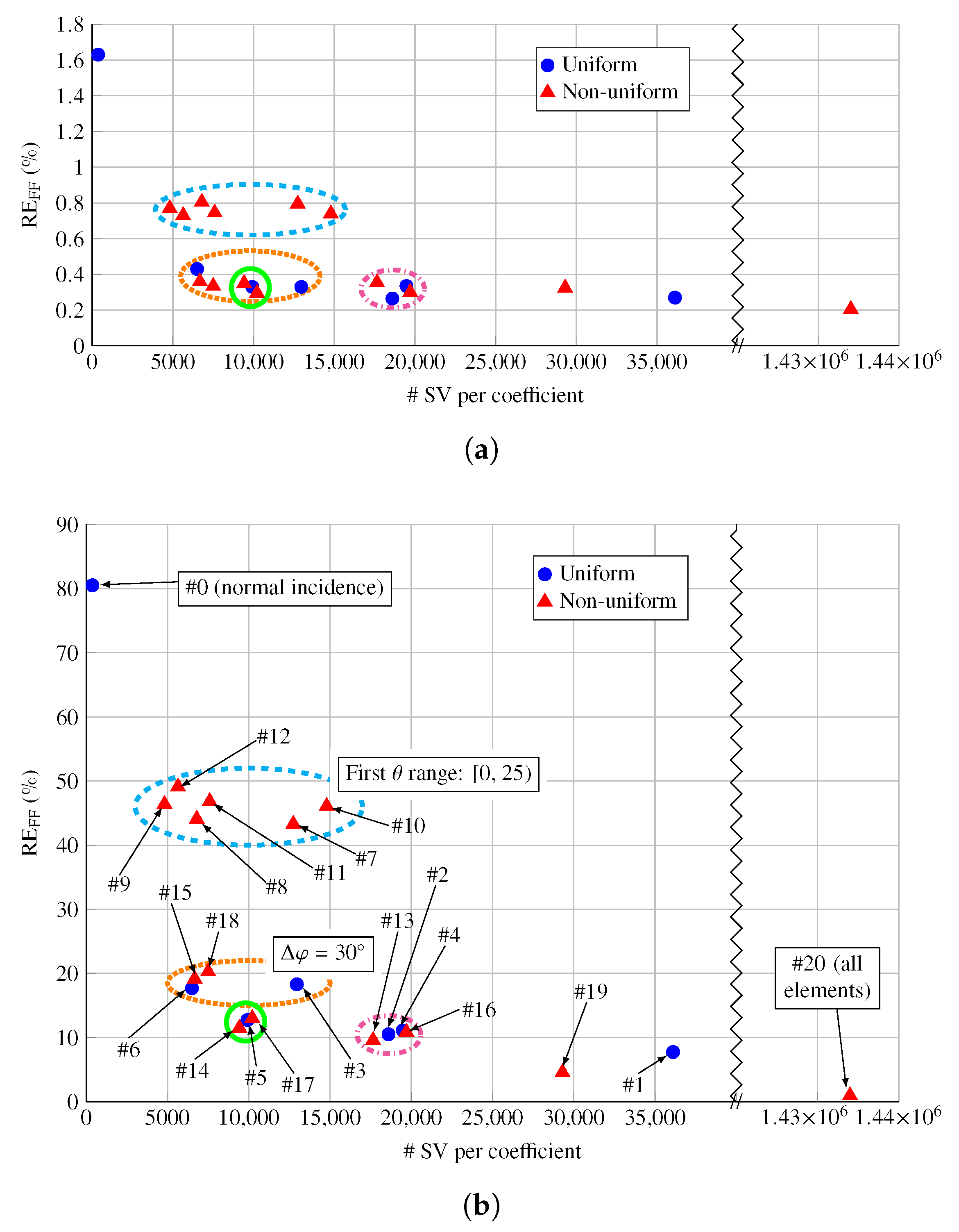
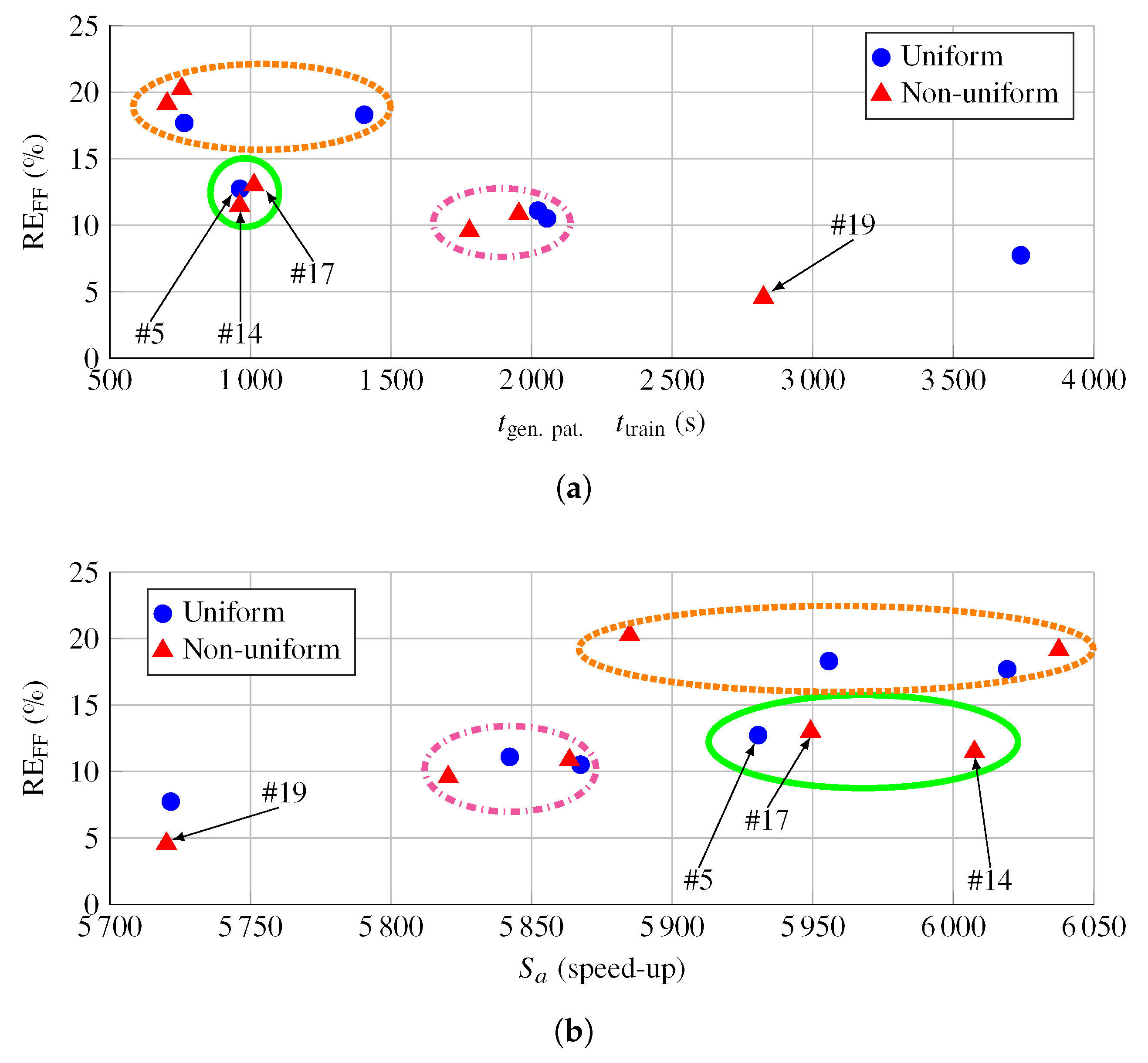
4.3. Analysis of the Results

Figure 5 shows the relative error for the copolar and crosspolar patterns calculated with (5) for the 21 discretizations of Table 2. The abscissa represents the total number of support vectors taking into account all the pairs of angles of incidence. In addition, only Figure 5b is tagged in order not to overload the figure, but clusters of points are grouped in colored ellipses for easy identifications. As can be seen, the error for the copolar pattern is very low, always below 1% with the exception of the normal incidence discretization, whose error is close to 1.6%. In addition, the error when all reflectarray elements have their own models is 0.2%. In this case, since the SVR models consider the real angle of incidence, the error is exclusively produced by the inherent SVR modeling and serves as benchmark for the rest. Attending to the copolar pattern error, we can distinguish between three groups of discretizations. First, the normal incidence, with the highest error of 1.6%. Then, six discretizations with an error around 0.7%, corresponding to Discretizations #7–#12. This group presents a coarse discretization of θ , with a first range grouping all elements with θ ( 0 , 25 ) . The rest of the discretizations show an error for the copolar pattern around 0.3%. This demonstrates that the copolar pattern is robust against the discretization of the angle of incidence, even when only employing normal incidence curves for reflectarray design. Finally, note the small sensitivity of the error to the discretization in φ .
The crosspolar pattern is more sensitive to the discretization and provides more relevant information. As can be seen, the crosspolar pattern is greatly affected by the coarse discretization of θ for normal incidence and the group of Discretizations #7–#12. In the latter case, the step in φ does not significantly alter the relative error. Once θ is properly discretized, the error drops significantly. There is another group comprised of discretizations with Δ φ = 30 , with a relative error around 20%. For finer discretizations of φ , the relative error only diminishes slightly while considerably increasing the total number of ( θ , φ ) pairs, as in Discretizations #1, #19 and #20. The lowest error is achieved when all reflectarray elements have their own model (#20), with a relative error of 0.97%. A good trade-off between the number of pairs and the relative error is given by Discretizations #5, #14 and #17, with 52 pairs in the three cases. Meanwhile, Discretization #19 is the most accurate among the eligible discretizations. Note that Discretization #20 (indeed, the most accurate) is only considered for reference, but it is not an eligible discretization since it presents too many angles of incidence.
Figure 6a shows the relative error versus the training time plus the time it takes to generate the training patterns. The time was measured in a workstation with two Intel Xeon E5-2650v3 CPU at 2.3 GHz and 256 GB of RAM. The sets with bad performance and with an unacceptable number of angle pairs are not shown. The arrangement between sets is similar to that shown in Figure 5. The sets of Discretizations #5 and #14 are slightly faster to train than Discretization #17, but they are still clustered together. The speed-up in reflectarray analysis ( S a ) vs. the relative error for the crosspolar pattern is shown in Figure 6b. This acceleration factor is calculated as:
S a = t ¯ an . MoM - LP t ¯ an . SVR ,
where t ¯ an . MoM - LP is the mean time that takes the MoM-LP to analyze a number of unit cells and t ¯ an . SVR is the mean time that takes the SVR-based model to analyze the same number of unit cells. All SVR present a similar speed-up. This happens due to the fact that, when analyzing the reflectarray, for each element only one ( θ , φ ) pair is used, and it turns out that the number of support vectors per coefficient and angle of incidence is approximately the same for all 2D SVR shown in Table 2.
In light of these results, Discretization #19 is the best since it presents the lowest error in the prediction of the crosspolar pattern while having an acceptable number of ( θ , φ ) pairs. In addition, Discretization #14 presents a good trade-off between computational efficiency and the achieved error. These two discretizations are selected for a comparison with MoM-LP simulations in the following section to visually assess their effect in the radiation pattern.

4.4. Further Discussion

From the results shown in Figure 5 and Figure 6, a few conclusions may be drawn. First, the copolar pattern is very robust against coarse discretizations of the angles of incidence, as shown in Figure 5a, where all the relative errors are below 1.7%. This is one of the reasons normal incidence-based designs usually work for the copolar pattern. The reason behind lies in the stability of the phase-shift curve of the direct reflection coefficients (see Figure 3), which is mainly responsible for the shape of the copolar pattern. However, this is not true for the crosspolar pattern, as shown in Figure 5b. In this case, the cross-coefficients present more variation with the angle of incidence (as shown in Figure 3), and, by not capturing this behavior with a finer discretization of θ , the crosspolar pattern will present a higher relative error. Thus, the second conclusion is that, to have a low relative error in the crosspolar pattern, a proper discretization of θ is necessary (as well as of φ ).
Finally, and as a rule of thumb, a uniform discretization in θ with steps Δ θ between 5 and 10 and in φ with steps Δ φ between 10 and 20 is enough, choosing the smaller values if more accuracy is necessary. Attending to Figure 5 and Table 2, choosing Δ θ = 5 and Δ φ = 10 is equivalent to Discretization #19, while choosing Δ θ = 10 and Δ φ = 20 is equivalent to Discretization #14. These values guarantee acceptable errors in the prediction of the radiation patterns, as shown in Section 5.

5. Effect of the Discretization on Several Radiation Patterns

According to the study carried out in Section 4, Discretization #19 (see Table 2) was selected because it presented the lowest error with an acceptable number of ( θ , φ ) pairs. In addition, Discretization #14 was also selected as a trade-off between computational efficiency and the achieved error. Table 3 summarizes the results of the achieved test error and training time for both discretizations. The average test error takes into account the error for all the angle of incidence pairs. As can be seen, both discretizations present similar test errors for the prediction of the reflection coefficients. This means that the differences in errors in the prediction of the radiation patterns are due to the discretization of the angles of incidence and not to the SVR models per se.
To graphically compare the different approaches, three radiation patterns are considered using the same antenna optics described in Section 4.2:
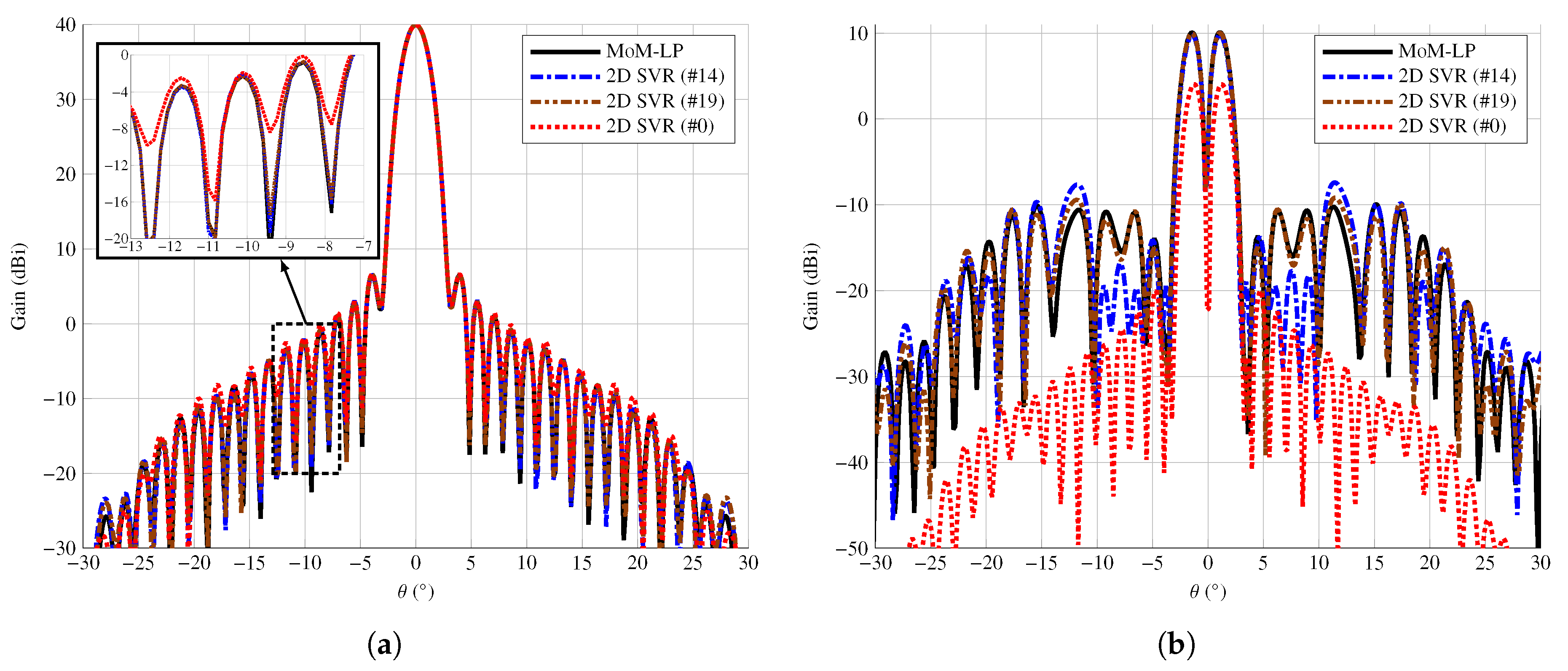
  • Pencil beam pattern in boresight direction.
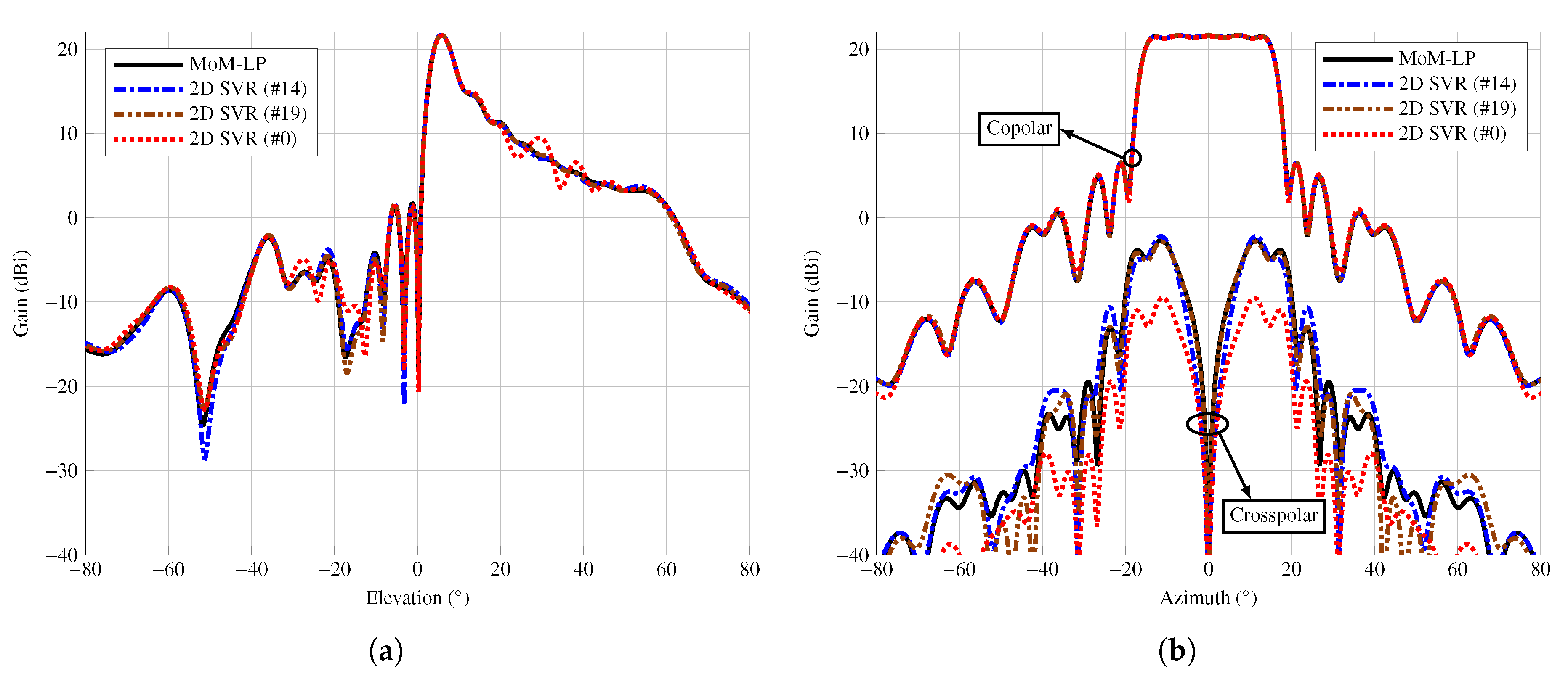
  • Shaped-beam reflectarray with a sectored beam pattern in azimuth and a squared-cosecant pattern in elevation. This radiation pattern presents a dynamic range in the coverage zone of almost 15 dB in elevation, where the copolar component has to smoothly decrease over an angular span of 50 .
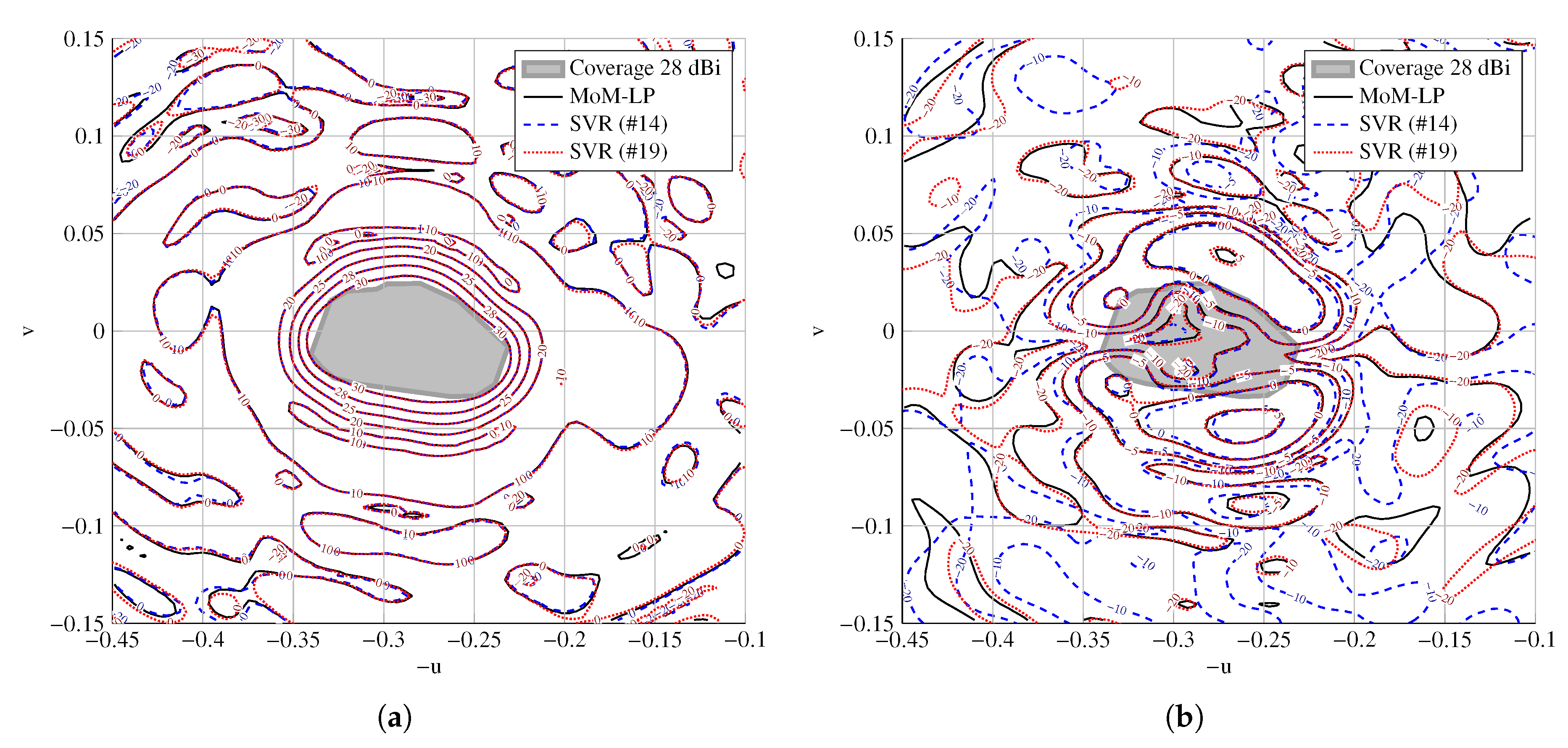
  • Contoured beam with European coverage for direct-to-home (DTH) applications. This kind of application has very tight cross-polarization requirements. Thus, it is necessary to accurately predict the crosspolar pattern. This is the same radiation pattern considered in previous sections.
For the three cases, a dual-linear reflectarray is designed following the steps detailed in [31]. Please note that, according to Figure 1, the vertical polarization (V) corresponds to the field aligned to the x ^ axis. In addition, the following tools are compared. The MoM-LP serves as the baseline. Then, in addition to Discretizations #14 and #19, Discretization #0, which corresponds to the normal incidence model, is also compared for the pencil and shaped-beam patterns.
For the pencil beam pattern, Figure 7 shows the main cut for φ = 90 for the copolar and crosspolar components of polarization V. The reference is the simulation performed with the MoM-LP tool, and it is compared with Discretizations #0, #14 and #19 (see Table 2). The simulation of the copolar pattern shows that all approaches give very similar results. In this case, there are some discrepancies for the normal incidence SVR model (Discretization #0) in some nulls (see the inset), which are not as deep as the ones predicted by the rest of SVR models. However, this model presents serious discrepancies in the prediction of the crosspolar pattern, giving a maximum value that is several dB below the real value. However, the other SVR models present a higher degree of accuracy with regard to the MoM-LP simulation. As expected, Discretization #19 presents a higher degree of accuracy for the prediction of the crosspolar pattern than Discretization #14.
Figure 8 shows the main cuts for the radiation pattern with squared-cosecant and sectored beams. The MoM-LP simulation is compared with the same SVR models as in the previous example (Discretizations #0, #14 and #19). The copolar pattern is predicted with a high degree of accuracy by the SVR Discretizations #14 and #19. However, the normal incidence model (Discretization #0) presents a ripple of around 5 dB in the coverage area in the same cut, but not in the cut in azimuth, where all models are very accurate. The SVR Discretization #0 presents the largest deviation with regard to the MoM-LP simulation, while the SVR Discretizations #14 and #19 present better accuracy than the normal incidence model, especially in the zone of maximum cross-polarization. Similar results were obtained for polarization H.
Figure 9 shows, for polarization V, the radiation pattern for the very large reflectarray with European coverage, comparing the MoM-LP simulation and the SVR Discretizations #14 and #19 predictions. As in the previous case, the accuracy in the prediction of the copolar pattern for both SVR is very high, with very slight discrepancies for the 0 dBi curves and below. Again, the SVR Discretization #19 is better for the prediction of the crosspolar pattern than SVR Discretization #14. However, both SVRs present high accuracy for the high levels of the crosspolar pattern. A 2D discretization such as Discretizations #14 may be employed, offering a similar accuracy in the copolar pattern, and with reasonable results in the critical parts of the crosspolar pattern (i.e., the areas with the highest gain).
Finally, Table 4 summarizes the errors obtained for the three radiation patterns for the different SVR models. As can be seen, the SVR Discretizations #14 and #19 offer lower error in the copolar pattern. The model for normal incidence presents an acceptable error for the copolar pattern but fails to predict the crosspolar pattern. In light of these results, it is clear that a proper discretization of the angles of incidence is necessary to obtain a good prediction of the crosspolar pattern. This is relevant for those applications in which the optimization of the cross-polarization performance is important.

6. Conclusions

In this study, we carried out a systematic investigation on how the discretization of the angles of incidence in reflectarray antennas affects the prediction of the radiation patterns. This study was applied to surrogate models of the reflectarray unit cell using support vector regression (SVR). As a baseline, simulations considering the real angle of incidence at each reflectarray element and a method of moments based on local periodicity (MoM-LP) were considered. The figure of merit was the relative error between the SVR prediction and MoM-LP simulation of the radiation pattern, considering both the copolar and crosspolar components in dual-linear polarized designs.
The results of this study showed that, in addition to the great stability of the copolar radiation pattern with the angle of incidence, the crosspolar component is very sensitive to the discretization of the angle of incidence. The physical explanation for this phenomenon lies in the electromagnetic response of the unit cell, i.e., the reflection coefficients, and their relation to the far field. On the one hand, the copolar pattern mainly depends on the direct coefficients ( ρ x x and ρ y y ), whose magnitude and phase are usually very stable with the angle of incidence of the impinging plane wave. As a consequence, the copolar pattern will be barely affected by the discretization of the angles of incidence. In fact, even considering normal incidence only, the cumulative error in the copolar pattern is less than 3%. This is the reason normal incidence curves are usually employed in the literature to perform reflectarray copolar design.
On the other hand, the crosspolar pattern depends on the four reflection coefficients, including the cross-coefficients ( ρ x y and ρ y x ). It was shown that the cross-coefficients strongly depend on the angles of incidence, and this dependence is directly translated into the crosspolar pattern. Thus, to correctly predict the crosspolar pattern, the discretization of the angles of incidence has to conveniently capture the behavior of the cross-coefficients. In this study, it was shown that a discretization in θ , with steps between 5 and 10 , and in φ between 10 and 20 is enough to properly predict the crosspolar pattern with a high degree of accuracy.
The results presented here are valuable as guidelines for the development of efficient tools for the design of reflectarray antennas. The main conclusions reached comprise two aspects. First, due to the curse of the dimensionality [15], it is more competitive to generate surrogate models per angle of incidence, as done in this work, rather than to include the angles of incidence as input variables and thus having models with higher dimensionality. However, the discretization of the angles of incidence may introduce distortions in the radiation pattern. In this regard, the present study showed that, while the copolar pattern is robust against the discretization, the crosspolar pattern is very sensitive. This is especially important for space applications with tight crosspolarization requirements. While it is true that reflectarray copolar design may be achieved with normal incidence curve, the optimization and correct prediction of the crosspolar pattern relies on a proper discretization of the angles of incidence, as shown in this study. Finally, these conclusions are also applicable to other types of antennas based on periodic and quasi-periodic surfaces such as transmitarrays, metasurfaces and phased-arrays.

Author Contributions

Conceptualization, D.R.P., J.A.L.-F. and M.A.; methodology, D.R.P. and J.A.L.-F.; software, D.R.P. and J.A.L.-F.; validation, D.R.P. and J.A.L.-F.; writing—original draft preparation, D.R.P.; writing—review and editing, D.R.P., J.A.L.-F. and M.A.; supervision, M.A.; project administration, M.A.; and funding acquisition, M.A. All authors have read and agreed to the published version of the manuscript.

Funding

This work was supported in part by the Ministerio de Ciencia, Innovación y Universidades under projects TEC2017-86619-R (ARTEINE) and IJC2018-035696-I; by the Ministerio de Economía, Industria y Competitividad under project TEC2016-75103-C2-1-R (MYRADA); and by the Gobierno del Principado de Asturias/FEDER under Project GRUPIN-IDI/2018/000191.

Acknowledgments

The authors thank R. Florencio, R. R. Boix and J. A. Encinar for providing the FW-LP software and Chih-Chung Chang and Chih-Jen Lin for making freely available the LIBSVM software.

Conflicts of Interest

The authors declare no conflict of interest.

Abbreviations

The following abbreviations are used in this manuscript:
ANNArtificial Neural Network
CPCopolar
DTHDirect-to-home
FW-LPFull-Wave analysis technique based on Local-Periodicity
MoM-LPMethod of Moments based on Local-Periodicity
SVMSupport Vector Machine
SVRSupport Vector Regression
XPCrosspolar

References

  1. Freni, A.; Mussetta, M.; Pirinoli, P. Neural network characterization of reflectarray antennas. Int. J. Antennas Propag. 2012, 2012, 1–10. [Google Scholar] [CrossRef]
  2. Robustillo, P.; Zapata, J.; Encinar, J.A.; Rubio, J. ANN Characterization of Multi-Layer Reflectarray Elements for Contoured-Beam Space Antennas in the Ku-Band. IEEE Trans. Antennas Propag. 2012, 60, 3205–3214. [Google Scholar] [CrossRef]
  3. Güneş, F.; Nesil, S.; Demirel, S. Design and Analysis of Minkowski Reflectarray Antenna Using 3-D CST Microwave Studio-Based Neural Network Model with Particle Swarm Optimization. Int. J. RF Microw. Comput. Eng. 2013, 23, 272–284. [Google Scholar] [CrossRef]
  4. Salucci, M.; Tenuti, L.; Oliveri, G.; Massa, A. Efficient Prediction of the EM Response of Reflectarray Antenna Elements by an Advanced Statistical Learning Method. IEEE Trans. Antennas Propag. 2018, 66, 3995–4007. [Google Scholar] [CrossRef]
  5. Prado, D.R.; López-Fernández, J.A.; Barquero, G.; Arrebola, M.; Las-Heras, F. Fast and Accurate Modeling of Dual-Polarized Reflectarray Unit Cells Using Support Vector Machines. IEEE Trans. Antennas Propag. 2018, 66, 1258–1270. [Google Scholar] [CrossRef]
  6. Shi, L.P.; Zhang, Q.H.; Zhang, S.H.; Liu, G.X.; Yi, C. Application of Machine Learning Method to the Prediction of EM Response of Reflectarray Antenna Elements. In Proceedings of the 2019 Photonics & Electromagnetics Research Symposium-Fall (PIERS-Fall), Xiamen, China, 17–20 December 2019; pp. 2671–2676. [Google Scholar] [CrossRef]
  7. Pozar, D.M.; Targonski, S.D.; Syrigos, H.D. Design of millimeter wave microstrip reflectarrays. IEEE Trans. Antennas Propag. 1997, 45, 287–296. [Google Scholar] [CrossRef]
  8. Huang, J.; Encinar, J.A. Reflectarray Antennas; John Wiley & Sons: Hoboken, NJ, USA, 2008. [Google Scholar]
  9. Johansson, F.S. A new planar grating-reflector antenna. IEEE Trans. Antennas Propag. 1990, 38, 1491–1495. [Google Scholar] [CrossRef]
  10. Cervellera, C.; Maccio, D. Learning With Kernel Smoothing Models and Low-Discrepancy Sampling. IEEE Trans. Neural Netw. Learn. Syst. 2013, 24, 504–509. [Google Scholar] [CrossRef]
  11. Chaharmir, M.R.; Shaker, J.; Legay, H. Broadband Design of a Single Layer Large Reflectarray Using Multi Cross Loop Elements. IEEE Trans. Antennas Propag. 2009, 57, 3363–3366. [Google Scholar] [CrossRef]
  12. Xue, F.; Wang, H.J.; Yi, M.; Liu, G.; Dong, X.C. Design of a Broadband Single-Layer Linearly Polarized Reflectarray Using Four-Arm Spiral Elements. IEEE Antennas Wireless Propag. Lett. 2017, 16, 696–699. [Google Scholar] [CrossRef]
  13. Nayeri, P.; Yang, F.; Elsherbeni, A.Z. Design of Single-Feed Reflectarray Antennas With Asymmetric Multiple Beams Using the Particle Swarm Optimization Method. IEEE Trans. Antennas Propag. 2013, 61, 4598–4605. [Google Scholar] [CrossRef]
  14. Prado, D.R.; López-Fernández, J.A.; Arrebola, M.; Goussetis, G. Support Vector Regression to Accelerate Design and Crosspolar Optimization of Shaped-Beam Reflectarray Antennas for Space Applications. IEEE Trans. Antennas Propag. 2019, 67, 1659–1668. [Google Scholar] [CrossRef] [Green Version]
  15. Prado, D.R.; López-Fernández, J.A.; Arrebola, M.; Goussetis, G. On the Use of the Angle of Incidence in Support Vector Regression Surrogate Models for Practical Reflectarray Design. IEEE Trans. Antennas Propag. 2020. [Google Scholar] [CrossRef]
  16. Prado, D.R.; Arrebola, M.; Pino, M.R.; Florencio, R.; Boix, R.R.; Encinar, J.A.; Las-Heras, F. Efficient Crosspolar Optimization of Shaped-Beam Dual-Polarized Reflectarrays Using Full-Wave Analysis for the Antenna Element Characterization. IEEE Trans. Antennas Propag. 2017, 65, 623–635. [Google Scholar] [CrossRef]
  17. Pozar, D.M.; Metzler, T.A. Analysis of a reflectarray antenna using microstrip patches of variable size. Electron. Lett. 1993, 29, 657–658. [Google Scholar] [CrossRef]
  18. Encinar, J.A.; Arrebola, M.; Dejus, M.; Jouve, C. Design of a 1-metre reflectarray for DBS application with 15% bandwidth. In Proceedings of the First European Conference on Antennas and Propagation (EuCAP), Nice, France, 6–10 November 2006; pp. 1–5. [Google Scholar] [CrossRef]
  19. Pozar, D.M.; Targonski, S.D.; Pokuls, R. A shaped-beam microstrip patch reflectarray. IEEE Trans. Antennas Propag. 1999, 47, 1167–1173. [Google Scholar] [CrossRef]
  20. Encinar, J.A. Design of a dual frequency reflectarray using microstrip stacked patches of variable size. Electron. Lett. 1996, 32, 1049–1050. [Google Scholar] [CrossRef]
  21. Encinar, J.A. Design of two-layer printed reflectarrays using patches of variable size. IEEE Trans. Antennas Propag. 2001, 49, 1403–1410. [Google Scholar] [CrossRef]
  22. Headland, D.; Carrascoo, E.; Nirantar, S.; Withayachumnankul, W.; Gutruf, P.; Schwarz, J.; Abbott, D.; Bhaskaran, M.; Sriram, S.; Perruisseau-Carrier, J.; et al. Dielectric Resonator Reflectarray as High-Efficiency Nonuniform Terahertz Metasurface. ACS Photonics 2016, 3, 1019–1026. [Google Scholar] [CrossRef]
  23. Zhou, M.; Sørensen, S.B.; Kim, O.S.; Jørgensen, E.; Meincke, P.; Breinbjerg, O. Direct Optimization of Printed Reflectarrays for Contoured Beam Satellite Antenna Applications. IEEE Trans. Antennas Propag. 2013, 61, 1995–2004. [Google Scholar] [CrossRef] [Green Version]
  24. Imaz-Lueje, B.; Prado, D.R.; Arrebola, M.; Pino, M.R. Reflectarray antennas: A smart solution for new generation satellite mega-constellations in space communications. Sci. Rep. 2020. [Google Scholar] [CrossRef]
  25. Vaquero, A.F.; Arrebola, M.; Pino, M.R.; Florencio, R.; Encinar, J.A. Demonstration of a Reflectarray with Near-field Amplitude and Phase Constraints as Compact Antenna Test Range Probe for 5G New Radio Devices. IEEE Trans. Antennas Propag. 2020. [Google Scholar] [CrossRef]
  26. Prado, D.R.; Arrebola, M.; Pino, M.R.; Goussetis, G. Contoured-Beam Dual-Band Dual-Linear Polarized Reflectarray Design Using a Multi-Objective Multi-Stage Optimization. IEEE Trans. Antennas Propag. 2020, 68, 7682–7687. [Google Scholar] [CrossRef]
  27. Chang, C.C.; Lin, C.J. LIBSVM: A library for support vector machines. ACM Trans. Intell. Syst. Technol. 2011, 2, 27:1–27:27. Available online: https://www.csie.ntu.edu.tw/~cjlin/libsvm (accessed on 24 September 2020). [CrossRef]
  28. Florencio, R.; Boix, R.R.; Encinar, J.A. Enhanced MoM Analysis of the Scattering by Periodic Strip Gratings in Multilayered Substrates. IEEE Trans. Antennas Propag. 2013, 61, 5088–5099. [Google Scholar] [CrossRef]
  29. Schölkopf, B.; Smola, A.J. Learning with Kernels, 1st ed.; The MIT Press: Cambridge, MA, USA, 2001. [Google Scholar]
  30. Platt, J.C. Sequential Minimal Optimization: A Fast Algorithm for Training Support Vector Machines; Technical Report MSR-TR-98-14; Microsoft Research: Redmond, WA, USA, 1998. [Google Scholar]
  31. Prado, D.R.; López-Fernández, J.A.; Arrebola, M.; Pino, M.R.; Goussetis, G. General Framework for the Efficient Optimization of Reflectarray Antennas for Contoured Beam Space Applications. IEEE Access 2018, 6, 72295–72310. [Google Scholar] [CrossRef]
  32. Prado, D.R.; López-Fernández, J.A.; Arrebola, M.; Pino, M.R.; Goussetis, G. Wideband Shaped-Beam Reflectarray Design Using Support Vector Regression Analysis. IEEE Antennas Wirel. Propag. Lett. 2019, 18, 2287–2291. [Google Scholar] [CrossRef]
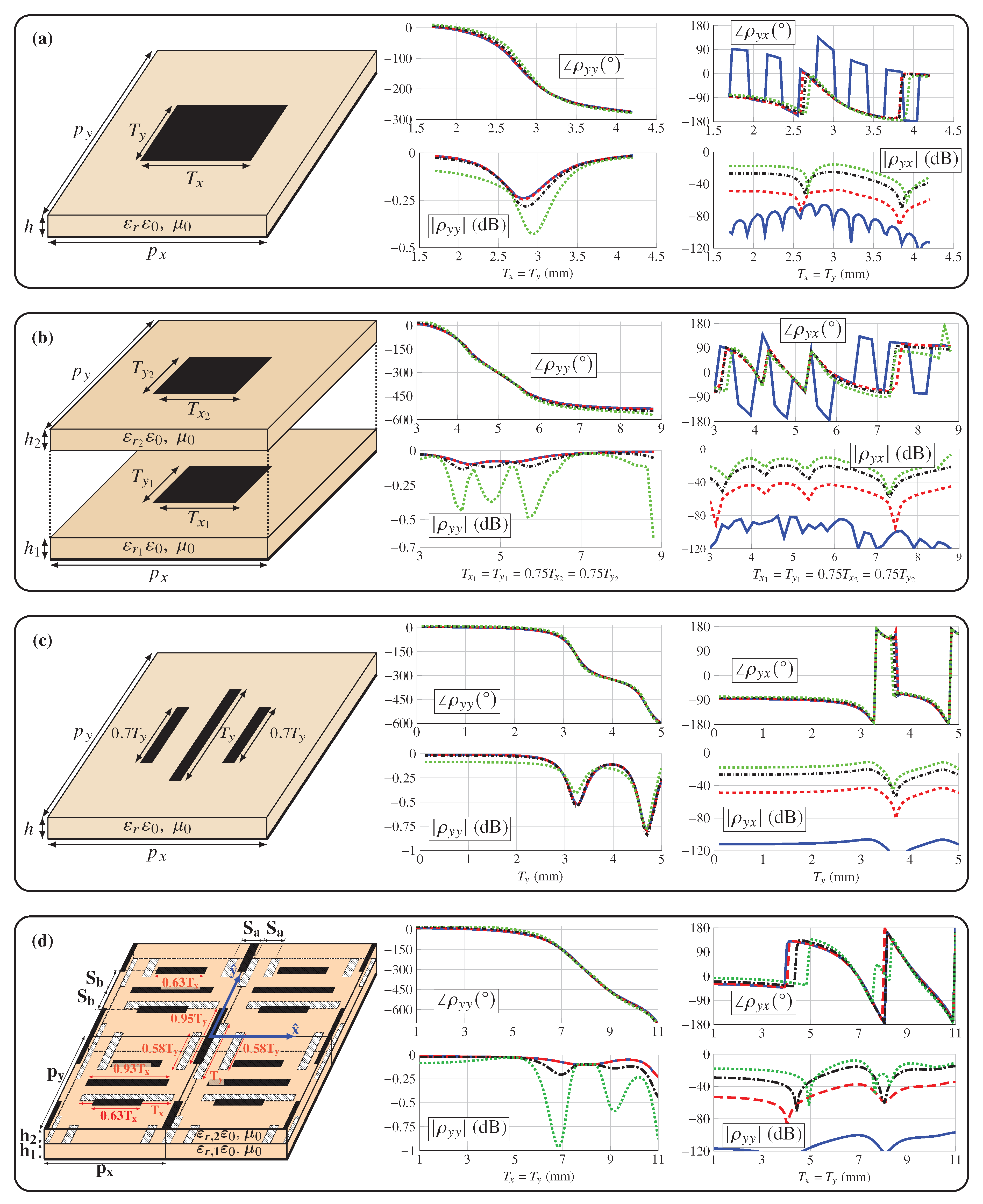
Figure 1. Sketch of a single-offset reflectarray configuration showing the definition of the angle of incidence ( θ , φ ) experienced by the kth element. The angle of incidence depends on the feed phase center position r f and the element coordinates ( x k , y y ) . For the kth element shown in this example, the value of φ k is negative since y k < 0 .
Electronics 09 02105 g001
Figure 2. Angle of incidence in degrees seen from each reflectarray element of an impinging wave coming from the feed: (a) θ ; and (b) φ .
Electronics 09 02105 g002
Figure 3. Electromagnetic response of several unit cells for the direct coefficient ρ y y and the cross-coefficient ρ y x : (a) single patch; (b) two stacked patches; (c) three parallel dipoles orientated in the y ^ axis; and (d) two sets of four parallel dipoles shifted half a period from each other ( S a = S b = 3.9 mm and dipole widths of 0.5 mm). The results are for oblique incidence at ( θ = 1 , φ = 1 ) (blue solid line), ( θ = 10 , φ = 15 ) (red dashed line), ( θ = 25 , φ = 40 ) (black dashed-dotted line) and ( θ = 40 , φ = 50 ) (green dotted line). Shared characteristics of the unit cells for the electromagnetic response shown here are described in Table 1. Some of these unit cells have been employed in other works for the design of reflectarray antennas. For instance, (b) is taken from [24], (c) from [25] and (d) from [26]. The results for a design using unit cell (a) are unpublished.
Electronics 09 02105 g003
Figure 4. Examples of: (a) uniform discretization in θ (Discretizations #4-#6 in Table 2); and (b) non-uniform discretization (Discretizations #7-#9 in Table 2).
Electronics 09 02105 g004
Figure 5. Relative error for the discretizations of the angles of incidence shown in Table 2 for the (a) copolar and (b) crosspolar patterns. There is a direct correspondence between the samples in both subfigures in the abscissa axis. Clusters of points are grouped in colored ellipses for easy identifications that share some common characteristics: dashed blue are coarse discretizations with a first θ range of 25 ; dotted orange are finer discretizations in θ with a step of Δ φ = 30 in φ ; solid green are discretizations with a trade-off between relative error and low number of support vectors per coefficients; and dashed dotted pink are discretizations with low error and a moderate number of support vectors per coefficient.
Electronics 09 02105 g005
Figure 6. Relative error of the crosspolar pattern for the discretizations of the angles of incidence shown in Table 2 versus: (a) the training time, t train , with the time it takes to generate the training patterns, t gen . pat ; and (b) the analysis speed-up. Times were measured in parallel mode. The same cluster of points as in Figure 5 are kept here for easy identification.
Electronics 09 02105 g006
Figure 7. Main cut of a pencil beam ( φ = 90 ) for the (a) copolar and (b) crosspolar radiation pattern for polarization V comparing the MoM-LP and SVR predictions.
Electronics 09 02105 g007
Figure 8. Main cuts for the copolar and crosspolar radiation pattern with (a) squared-cosecant pattern in elevation and (b) sectored beam in azimuth for polarization V comparing the MoM-LP and SVR predictions.
Electronics 09 02105 g008
Figure 9. Comparison of the MoM-LP simulation and SVR predictions for the (a) copolar and (b) crosspolar patterns for polarization V of a very large reflectarray with European coverage for DTH application.
Electronics 09 02105 g009
Table 1. Characteristics of the unit cells shown in  Figure 3.
Unit CellFrequencyPeriodicity ( p x = p y ) Substrate Characteristics
Relative PermittivityLoss TangentThickness
 Figure 3a28 GHz4.29 mm ε r = 2.3 tan δ = 0.005 h = 0.762 mm
( 0.4 λ 0 )
 Figure 3b17 GHz8.82 mm ε r 1 = 3 tan δ 1 = 0.001 h 1 = 0.762 mm
( 0.5 λ 0 ) ε r 2 = 3 tan δ 2 = 0.001 h 2 = 1.524 mm
 Figure 3c29 GHz5.0 mm ε r = 2.3 tan δ = 0.005 h = 0.762 mm
( 0.48 λ 0 )
 Figure 3d11.85 GHz12.0 mm ε r 1 = 2.55 tan δ 1 = 0.0009 h 1 = 2.363 mm
( 0.47 λ 0 ) ε r 2 = 2.17 tan δ 2 = 0.0009 h 2 = 1.500 mm
Table 2. Data regarding the discretization of the angles of incidence. Type refers to the discretization of θ (N, normal incidence; U, uniform; NU, non-uniform).
#Type Δ θ ( ) θ Set ( ) Δ φ ( ) θ , φ Pairs
0NI-{0}-1
1U5{2, 7, 12, 17, 22, 27, 32, 37}10190
2U5{2, 7, 12, 17, 22, 27, 32, 37}2098
3U5{2, 7, 12, 17, 22, 27, 32, 37}3068
4U10{5, 15, 25, 35}10102
5U10{5, 15, 25, 35}2052
6U10{5, 15, 25, 35}3034
7NU-{12, 29, 36}1064
8NU-{12, 29, 36}2034
9NU-{12, 29, 36}3024
10NU-{12, 27, 32, 37}1074
11NU-{12, 27, 32, 37}2038
12NU-{12, 27, 32, 37}3028
13NU-{7, 20, 29, 36}1090
14NU-{7, 20, 29, 36}2052
15NU-{7, 20, 29, 36}3034
16NU-{7, 20, 27, 32, 37}10100
17NU-{7, 20, 27, 32, 37}2052
18NU-{7, 20, 27, 32, 37}3038
19NU-{5, 10, 17, 23, 29, 35, 40}10152
20NUSurrogate models for all reflectarray elements7052
Table 3. Average relative error over the test set and training time of the SVR model with N r = 0.7 N for each output variable. N for Discretization #14 is 65,000, while for 2D SVR Discretization #19 is 190,000. The average test error RE ¯ SVR is in dB while the training time t train is in seconds.
SVRVariable ρ xx ρ yy Re { ρ xx } Im { ρ xx } Re { ρ xy } Im { ρ xy } Re { ρ yx } Im { ρ yx } Re { ρ yy } Im { ρ yy }
#14 RE ¯ SVR −81.7−82.0−38.1−38.5−39.2−38.6−38.3−38.4−38.6−38.7
#19 RE ¯ SVR −82.4−82.5−38.1−38.5−39.2−38.7−38.2−38.3−38.6−38.7
#14 t train 6456891 0191 0279169789901 192838961
#19 t train 1 8332 1223 0673 1752 7993 0442 9853 5862 4572 823
Table 4. Cumulative relative errors (%) in the prediction of the three radiation patterns using different SVR models for the copolar (CP) and crosspolar (XP) patterns.
DiscretizationPencil BeamShaped-BeamContoured-Beam
CPXPCPXPCPXP
#01.0278.132.5482.181.6380.52
#140.117.200.918.320.3611.54
#190.212.140.913.470.514.00
Publisher’s Note: MDPI stays neutral with regard to jurisdictional claims in published maps and institutional affiliations.

