1. Introduction
With the rapid development of automobile technology, car ownership has increased rapidly over the past decades. However, the frequent occurrence of road traffic accidents has brought social problems that seriously threaten the safety of human life and property. According to the data of World Health Organization [
1], more than 1.2 million people have died in traffic accidents each year, and millions were injured or maimed. Due to the increase in the number of traffic accidents, the severity of this problem has drawn considerable attention from society and governments [
2]. Therefore, how to prevent traffic accidents has become one of the most important aspects in the world. According to relevant research, traffic accidents caused by fatigue driving (FD) account for 20–30% of all traffic accidents, which indicates that FD is a major cause of traffic accidents [
3]. Drivers normally tend to be distracted, have less activity and slower brain response under fatigue, which will increase the likelihood of traffic accidents [
4]. FD detection (FDD) techniques have broad development prospects in the prevention of traffic accidents, and has gradually attracted intensive attention among researchers, automotive industry as well as government organizations.
Researchers have found that drivers’ physiological or driving behaviors can change drastically over a period of time before the accidents caused by FD happen [
5]. Based on these changes, many researchers have done some related researches and various methods have been proposed to detect FD, which can be classified into three categories: (1) detecting driver’s physiological information, e.g., electroencephalogram (EEG) [
6], electrocardiogram (ECG) [
7], electrooculogram (EOG) [
8], electromyography (EMG) [
9], respiratory signal and heart rate variability [
10]; (2) detecting driver’s physical behavior, such as eye state [
11], eye blink [
12] and gaze direction [
13], yawning [
14] and head movements [
15]; (3) detecting vehicle status and parameter, including lane position, steering wheel angle (SWA), driving speed, acceleration and braking [
16,
17,
18,
19,
20].
The driver’s physiological signals are highly reliable, with small error and little external interference in responding to the level of fatigue, because it can truly reflect the conditions inside the driver’s body. Dong et al. obtained EEG signals through electrodes embedded in the human head, and analyzed these signals to determine whether the driver is in a fatigue state [
21]. Wang et al. analyzed the fusion entropy combining EOG and EEG signals to detect the fatigue state of the driver [
22]. Changes in respiration and heartbeat signals have been reported to be associated with driver fatigue and the corresponding detection systems have been developed [
23]. However, in order to obtain the driver’s physiological signal, the existing detection methods and devices are normally invasive or contactable [
24]. Electrodes need to be attached to drivers, which is unacceptable for many users [
25].
Driver behavior based-detection technology has an important advantage that the detection is performed in a non-contact manner without causing interference to the driver, compared with the physiological signal detection method. The main work is to use the camera to obtain the driver’s facial condition and head movements, and use computer vision technology to determine the fatigue state [
26]. Cheng et al. collected the videos of 21 participants’ faces and extract many features including number of yawns, blink rate, statistics of blink duration, closing speed, reopening speed and so on, for establishing an FD assessment model [
27]. However, these methods are only applicable to the FD late stage, particularly when the driver’s facial changes are obvious and the driving behavior changes have reached a very dangerous stage. In addition, these technologies are also sensitive to external factors, such as driver wearing sunglasses or changes in brightness.
Vehicle parameter-based detection technology also exhibits the advantage of non-contact and is more suitable for real-time systems. However, this technology also has certain limitations. (i) In lane departure detection, road image data need to be captured and processed in real time, which results in the high cost of hardware and computer support development. (ii) Lane shift detection relies purely on external factors such as road markings, weather and light conditions. Although steering wheel detection seems to be a reliable alternative due to its low price and accurate detection without relying on external conditions [
28], steering wheel detection is only applicable under very limited conditions, because it is closely related to vehicle type, driver experience, and driver’s condition.
After obtaining a large amount of data through the above methods, they need to be well processed for better determining the driver’s fatigue level. Data processing methods are implemented via mathematical models and machine learning. The machine learning-based implementation method is to train a large amount of driving data obtained from the laboratory and the road, which is called a data-driven algorithm [
29]. At present, some researchers have made relevant explorations. Support vector machine (SVM) is a classic kernel learning method which aims to find the best hyperplane to maximize the margin [
30]. Hu and Zheng extracted the eyelid-related parameters from the electrooculogram (EOG) as the data input, and utilized SVM to classify the driver state into alert, sleepy and very sleepy [
31]. The disadvantage of SVM lies in that it cannot directly support multi-classification and it has difficulties in training large-scale data. The back propagation neural network (BPNN) is a multilayer feedforward neural network trained using the error back propagation algorithm [
32], which has been widely used in driver fatigue detection. Ying et al. obtained the relevant parameters of eyes and mouth from the driver’s entire face image as data input and then adopted the BPNN to judge the fatigue state [
33]. However, BPNN has significant drawbacks, such as slow convergence speed, many adjustable parameters, and falling into local minimums, which leads to training failure.
Recently, in the field of classifications, in addition to some typical machine learning algorithms, i.e., enhanced k-NN [
34], random forests [
35], extreme learning machine (ELM) as a new type of single-layer feedforward network (SLFN) learning algorithm has attracted a great deal of attention among researchers. Different from BPNN, ELM has the advantages of faster learning speed, easier modeling, and better generalization performance [
36,
37,
38], which has a great potential to be applied in FDD. However, the random selection of the input weights and hidden thresholds might greatly affect the accuracy of ELM classification. Considering the fact that the differential evolution (DE) algorithm has the characteristics of simple structure, easy implementation, fast convergence and strong robustness [
39], the DE algorithm can be used to optimize the initial weights and biases in traditional ELM, which can increase the sensitivity of neurons, obtain the optimal network model, and thereby improve the classification accuracy. The differential evolution extreme learning machine (DE-ELM) algorithm was successfully applied to analog circuit fault diagnosis [
40].
Considering the above problems of FDD and motived by ELM and DE, in this paper, we use Doppler radar and smart bracelets to collect the driver’s respiration and heartbeat signals, and then develop an FDD method based on DE-ELM. The rest of this paper is organized as follows. In
Section 2, the designed human respiratory and heartbeat signal detection platform and signal acquisition are given.
Section 3 introduces the process of data collection, the sample database establishment and classification. In
Section 4, DE-ELM-based FDD approach is developed in order to select the best weights and biases of the ELM. In
Section 5, experimental results are presented involving traditional ELM, DE-ELM and SVM classification accuracy of fatigue driving samples.
Section 6 draws the conclusion.
2. Experimental Platform
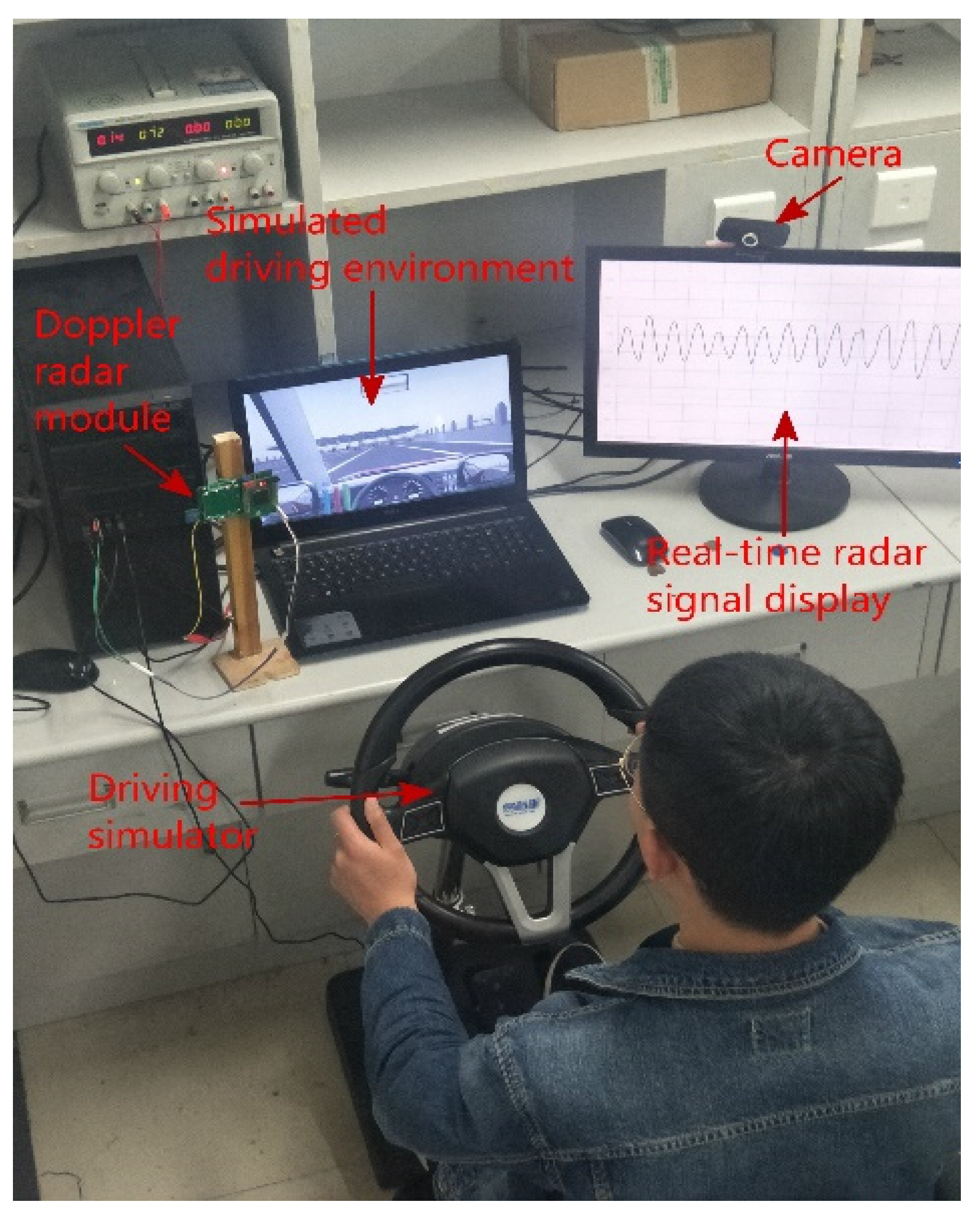
The experimental platform for the collection of respiratory and heartbeat signals in this paper is shown in
Figure 1. The platform mainly includes three parts: simulated driving system, physiological signal detection system and video signal acquisition system. The simulated driving system consists of two parts: a simulated driving device and a simulated driving environment reproduction system. The simulated driver device includes steering wheel, manual gear, clutch, throttle, brake, etc., while the simulated driving environment reproduction system uses a computer monitor to display the virtual driving environment. The driving simulation software adopts Yijiaxing driving simulation system, and the scenes are taken from on-site video images, such as from urban areas, residential areas, highways, and snowy environments. The front of the screen shows the virtual driving environment, traffic conditions, traffic lights, traffic signs, weather conditions, etc. The information of the car dashboard is displayed at the bottom of the screen. Additionally, physiological signal detection system is used to collect respiratory and heartbeat signals of drivers, video signal acquisition system is used to collect facial information of drivers, and video information serves as an important component for experts to judge fatigue level.
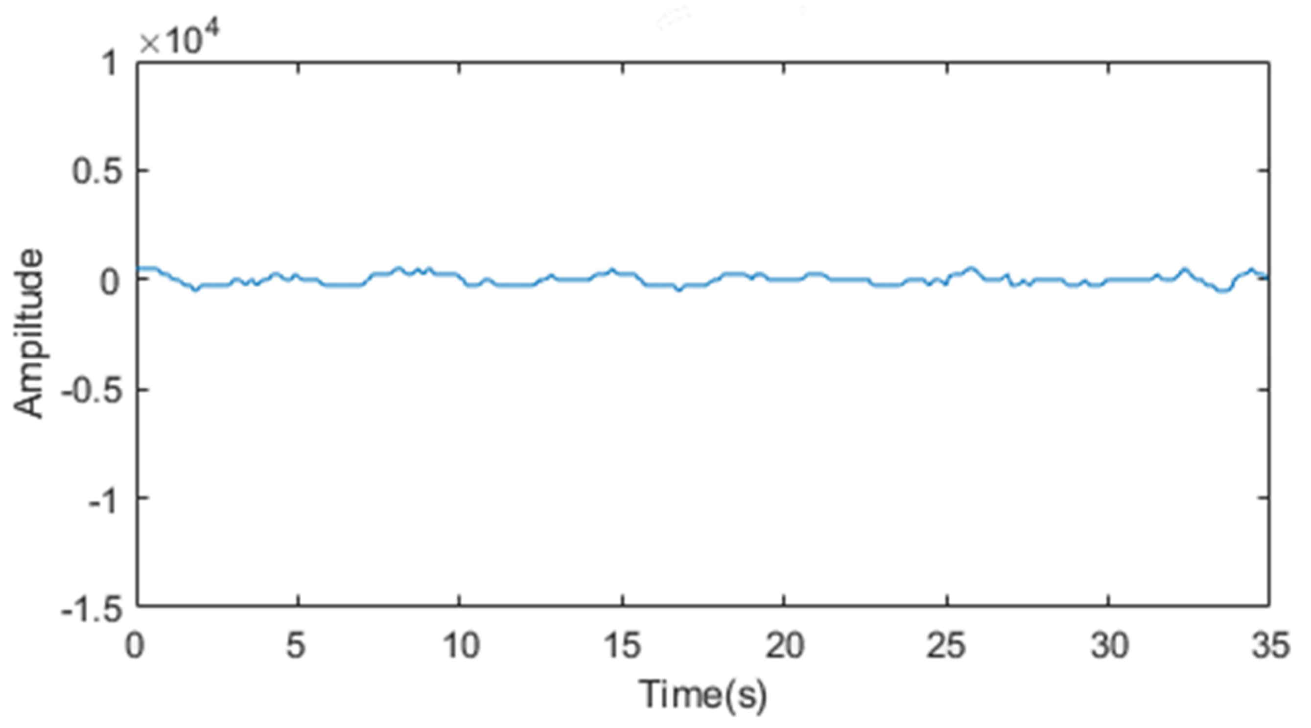
Based on the experimental platform, a set of data collected from the platform have been tested. The corresponding test results are described as follows: (i) the waveform shown in
Figure 2 is the signal collected by the radar module without testers. As is seen from the waveform, there is no signal input other than a small amount of noise signal. (ii) The waveform shown in
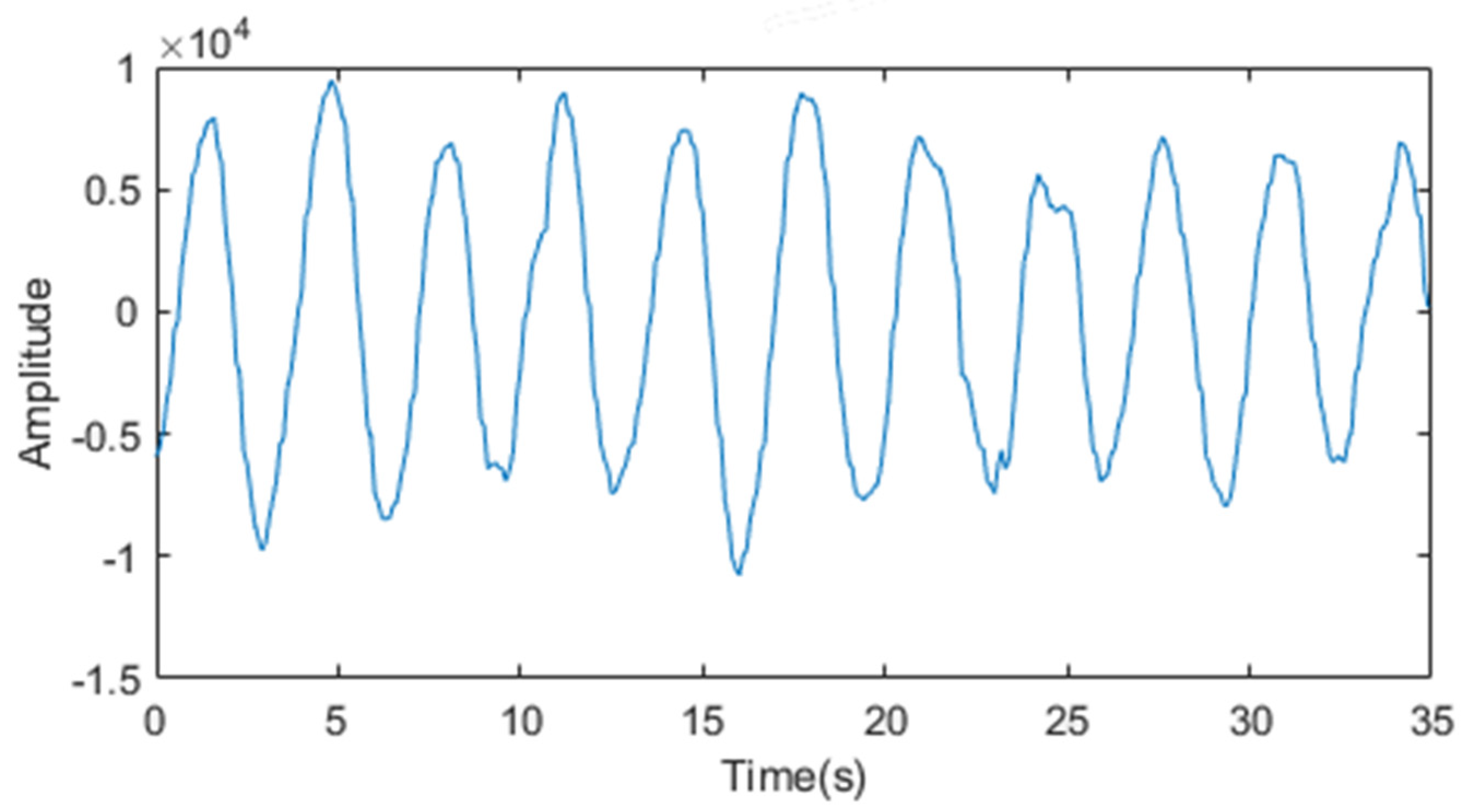
Figure 3 is the signal collected by the radar module with the tester breathing normally. As observed from the waveform, the waveform changes periodically and the signal should be composed of the respiratory signal, the heartbeat signal, and the noise superposition in each cycle. (iii) The waveform shown in
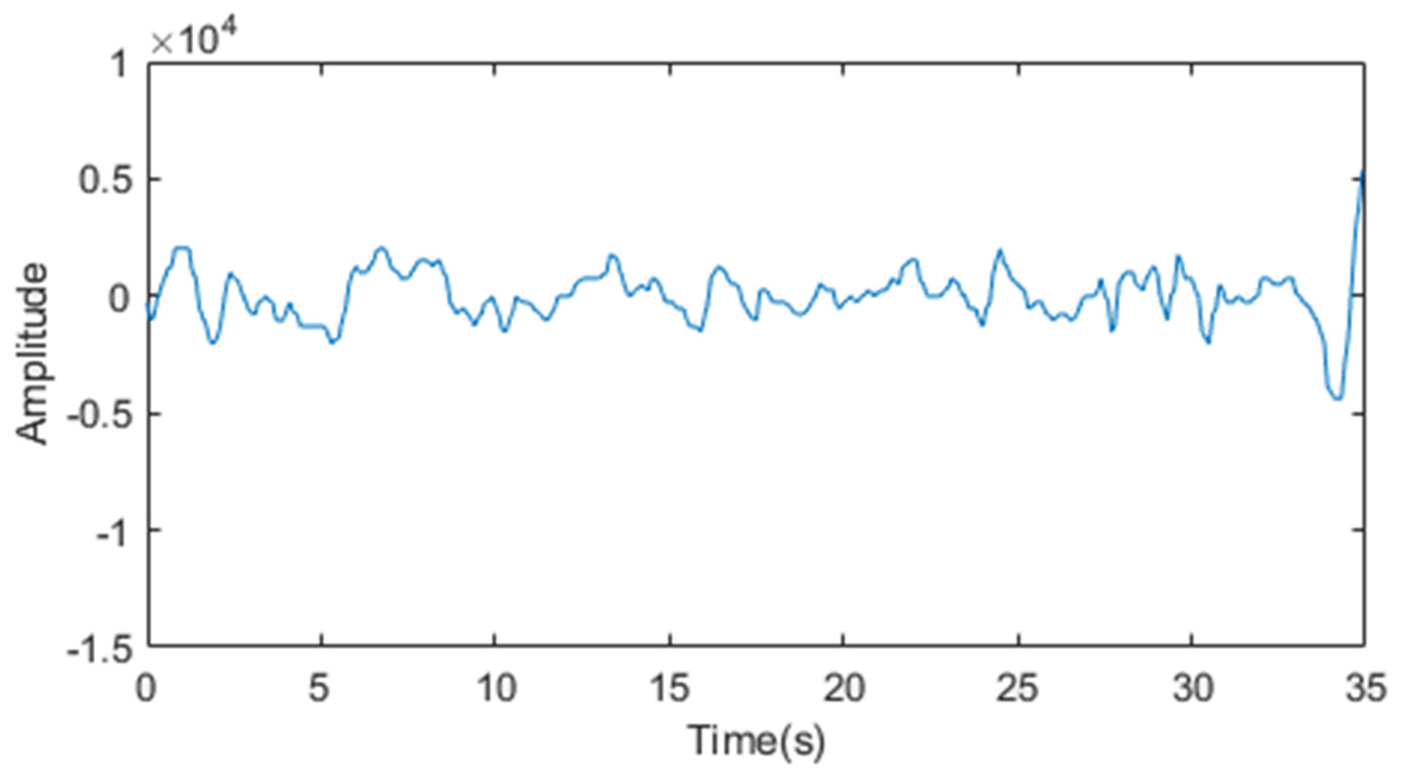
Figure 4 is the signal collected by the tester when he holds his breath. It can be seen that the amplitude of signal change is very small, which indicates that the heartbeat signal collected by the radar module is very weak as well as mixed with noise. Therefore, during signal collection, a smart bracelet is added to detect the driver’s heartbeat signal in real time which will be recorded every 2 min.
Through the above tests, it is noted that the Doppler radar module is used to detect human respiratory signals. As for the heartbeat signal, several experiments have shown that the heartbeat signal is very weak and is basically covered by noise, such that the Doppler radar module cannot detect the heartbeat signal. Instead, the smart bracelet is used for heart rate collection. The experiment recruited 7 drivers as experimental test subjects, including 6 men and 1 woman, aged between 22 and 30 years old. It requires good health, normal hearing and vision, and no red–green color blindness. Before the experiment, the tester is required to ensure sufficient sleep time. After the debugging of the whole experimental platform, the test personnel will conduct simulated driving, and each test period will last for 3 h. Throughout the three-hour test, the tester will experience different fatigue states. The Doppler radar module and the smart bracelet collect respiratory and heartbeat signals, and synchronizes video signals to record facial features. At the end of each test, a data set containing respiration and heartbeat signals and corresponding video signals will be obtained through each test. The entire data set will be used for the next expert’s review before classification into different fatigue levels.
3. Sample Library
In
Section 2, the data are classified through the facial expert evaluation method. This method was first introduced to the driver’s fatigue assessment and becomes the most practical method for evaluating the fatigue state of drivers [
41]. The specific operation procedure is as follows. Firstly, the video signals and the synchronously collected radar and smart bracelet signals are segmented every 2 min and stored randomly. Secondly, three facial experts are selected to score based on multiple indicators such as the rubbing eyes, scratching face, yawning, closing eyes, and adjusting postures, etc. The evaluation result is a continuous value between 0 and 3. The specific classification criteria are described in
Table 1. If more than two facial experts judge the same on a certain fatigue level, then the corresponding fatigue level of the driver in the video signal is determined. If the evaluation levels of the three experts are different, then the fatigue level evaluation of this signal needs to be re-evaluated. Finally, three experts will discuss and determine the fatigue level. After the fatigue level is determined, the signals need to be labeled for subsequent neural network learning. The video evaluation results are corresponding to the synchronous radar signals and the smart bracelet signals, which are used as the criteria and basis for fatigue driving evaluation.
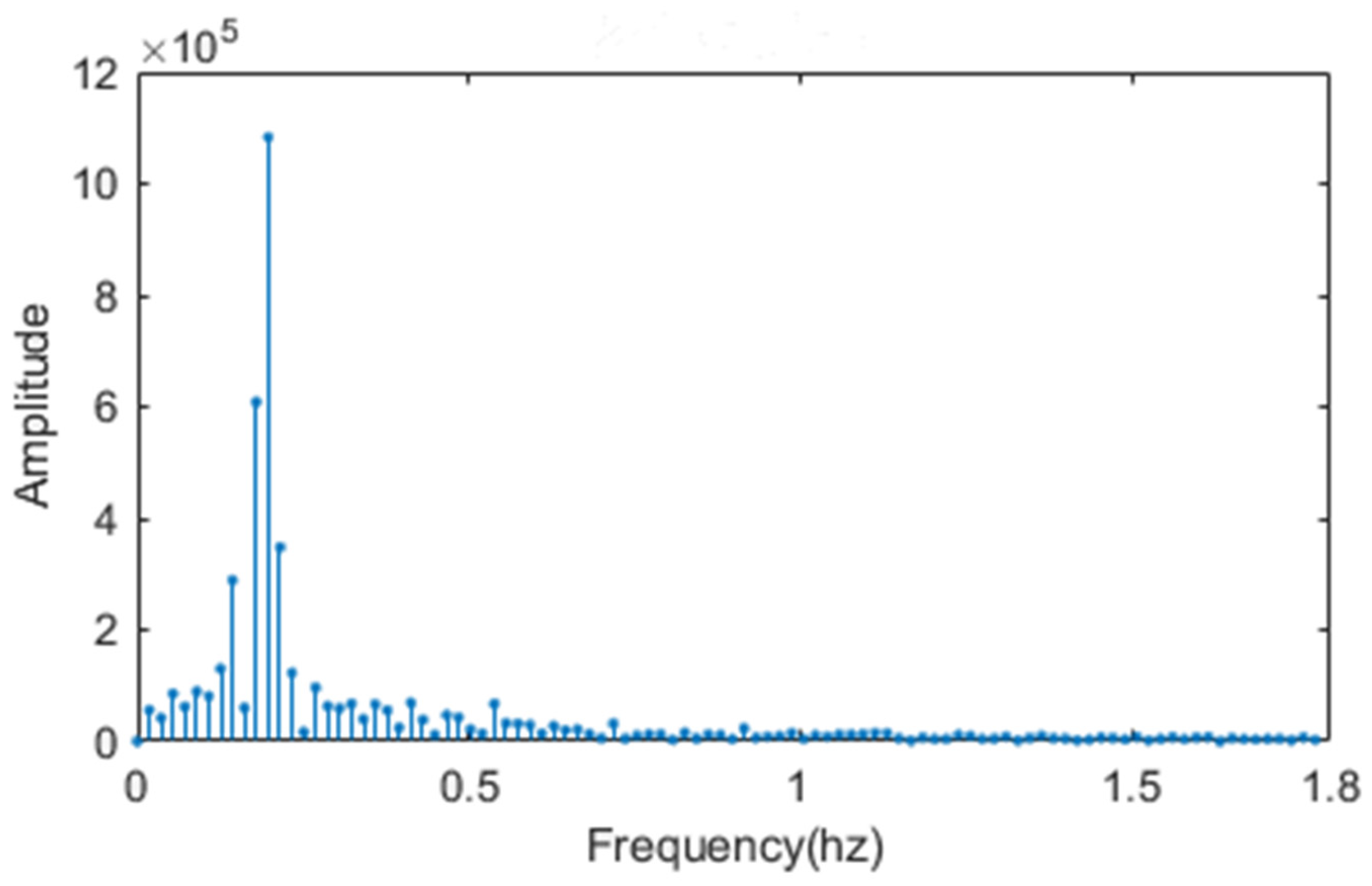
After classifying all signals according to the expert evaluation mechanism, it is necessary to conduct filtering processing and discrete Fourier transform (DFT) for each group of data. A zero-phase indefinite impulse response (IIR) filter is used for the filtering algorithm, which can completely eliminate the signal phase distortion and improve the real-time performance of detection at the cost of increasing the appropriate computation [
42]. After the filtering is completed, DFT processing of the signal will continue to obtain the spectrum diagram. Then, both the frequency and amplitude of the signal are extracted.
Figure 3 and
Figure 5 show the respiratory signal and its amplitude–frequency characteristics, respectively.
Finally, the following characteristic values are determined as the training sample data: , , , where is the respiratory cycle, is the respiratory amplitude, and indicates the heart rate.
The sample library can be built as:
where
X: input data.
T: output label corresponding to X.
h(x): impact function which defined as:
where
is the fatigue state with the value as 1, 2, 3 or 4, which correspondingly represents sober state, first-level fatigue state, second-level fatigue state and third-level fatigue state,
is the sample index, and
is the total sample size. A total of 720 sets of respiration and heartbeat data were collected in this experiment.
After obtaining the complete data set , we also need to divide it into training set and test set by using a subject-wise method. Data classification should follow the following three principles: (i) randomly assigned, (ii) training set sample size: test set sample size = 7:3, and (iii) the same number of samples per fatigue level.
In the following section, we will introduce the basic principles of ELM and DE-ELM in detail and further give the DE-ELM-based FDD approach.
4. Introduction of Classification Method
4.1. Extreme Learning Machine
ELM is an SLFN proposed by Guangbin Huang [
43], which consists of the following parts: dimension of input feature vector
n, total number of samples
N, number of hidden layer neurons
L, and dimension of outputs
m, data set
. It can be represented by following matrix:
Hidden layer input weight matrix is
:
Hidden layer output weight matrix is
:
The activation function selected in this paper is sigmoid function which is defined as:
By using the activation function, the nonlinear characteristics can be added to make learning faster and more efficient [
44]. Thus, we have
The output
can be expressed as:
The goal of the neural network learning is to minimize the output error
That is, there exist
,
and
, such that:
For the entire training set, Equation (17) can be expressed in matrix form as:
where
H is the hidden layer output matrix:
For fixed input weights and the hidden layer biases, to train an SLFN is simply equivalent to find a least-squares solution
of the linear system
:
According to the minimum norm criterion, the solution is obtained by finding the least squares:
where
is the Moore–Penrose generalized inverse of the hidden layer output matrix
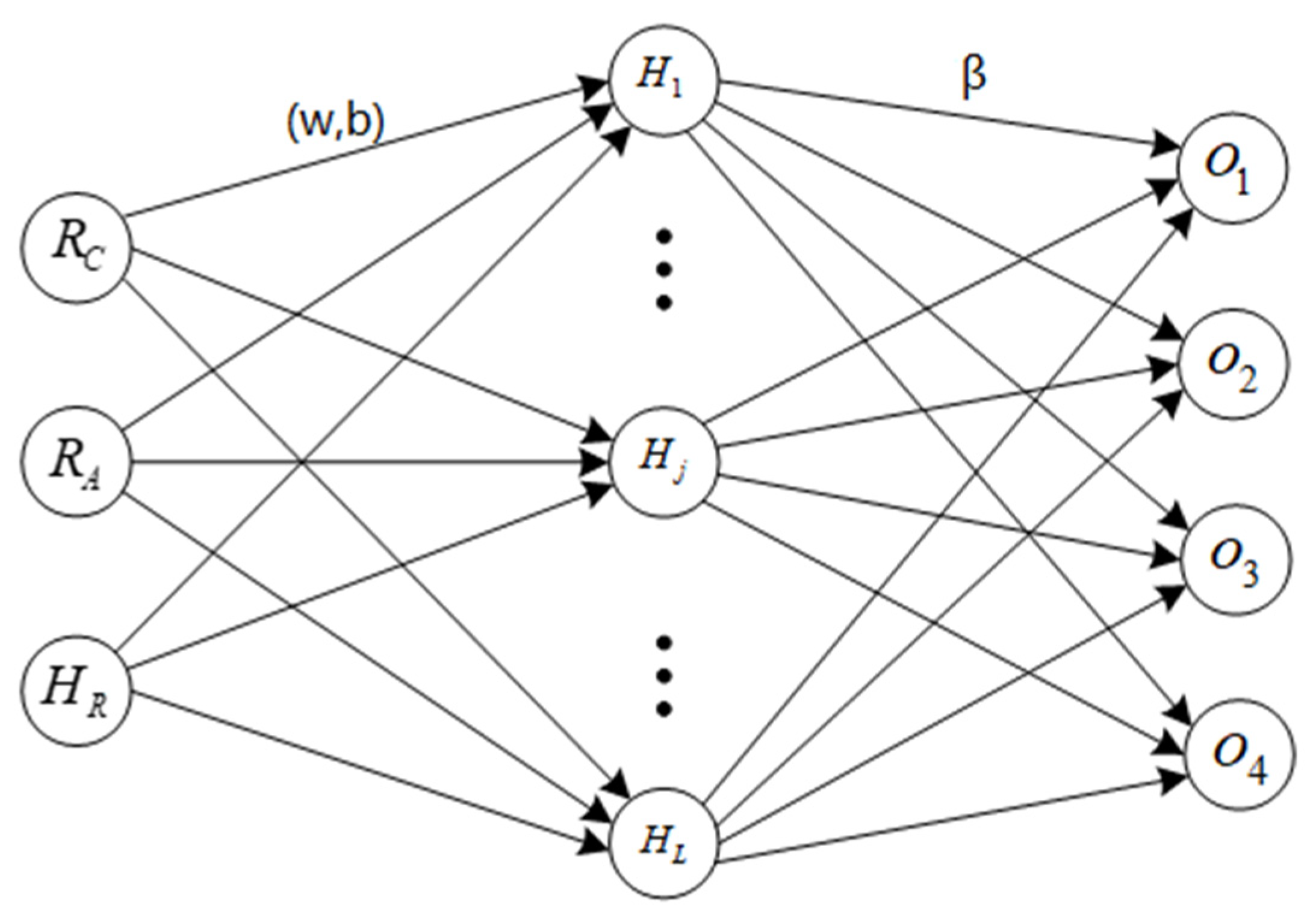
. In summary, when inputting training data and randomly initializing the input weight matrix, the output weight matrix can be obtained through Equation (22). The design of the ELM neural network model for fatigue driving detection is shown
Figure 6. It is noted that the ELM possesses the advantages of high learning efficiency and strong generalization ability and thus is widely used in classification, regression, clustering, feature learning and other problems [
45]. Since the input weights and the hidden layer biases of the ELM are randomly assigned, these weights and biases may not be the optimal choices relative to the input data. For practical applications, in order to enable the neural network to have better generalization performance, more hidden layer neurons may be needed, thereby increasing the complexity of the network. To compensate for these shortcomings, we will introduce differential evolution algorithms in the following section to optimize the weights and biases of the ELM, such that the optimal network structure can be obtained.
4.2. Differential Evolution ELM (DE-ELM)
Differential evolution, proposed by Storn and Price in 1995, is a simple yet powerful evolutionary algorithm (EA) [
39]. The basic idea of the optimization algorithm is as follows: starting from a randomly generated initial population, a new individual is generated by summing the vector difference of any two individuals in the population with a third individual, and then comparing the new individual with the corresponding individual in the contemporary population. The corresponding fitness is better than the fitness of the current individual, so the new individual will replace the old individual in the next generation, otherwise the old individual will still be saved. Through continuous evolution, it will keep the good individuals, eliminate the bad individuals, and guide the search to the optimal solution. Compared with most of the available evolutionary algorithms, it exhibits the advantages of simple structure, fast convergence, few adjustable parameters, and strong robustness, etc.
Next, we show the detailed mathematical description of DE algorithm in the following.
Step 1: Initialization. We randomly generate
individuals to form the primary population, where
is the dimension of the population. The
i-th individual
in the
g-th iteration can be marked as:
The value of the
j-th dimension of the
i-th individual
can be obtained by the following equation:
where
and
represent the upper and lower bounds of each parameter:
and
represents a random number uniformly distributed in the interval (0,1).
Step 2: Individual Evaluation. In this step, the entire population is evaluated, that is, the fitness function value of each individual in the population is calculated.
Step 3: Mutation Operation. DE achieves the mutation of individuals through a differential strategy, which is also an important difference from genetic algorithms. The differential strategy used in this paper is to randomly select two different individuals in the population, scale their vector differences, and perform vector synthesis with the individuals that need to be mutated, that is:
where
,
,
are randomly chosen in the range
, with
,
is the differential variation,
is the new mutation individual, and the constant factor
is a scaling parameter, which is used to control the amplification of the differential variation.
In the mutation process, in order to ensure the validity of the solution, it must be determined whether the parameters of each individual are between the maximum and minimum values. If this condition is not met, they will be regenerated by using Equation (24).
Step 4: Crossover Operation. The crossover to differential evolution algorithm is introduced for the sake of increasing the diversity of generation. Crossover operation is described as follows:
where
is the crossover probability and
is a random integer generated in the set
.
Step 5: Selection Operation. The purpose of this step is to generate individuals of the population in
generation. Among the target individual
and
obtained in the previous step, the one with better effect is selected as the individual
of the
generation population according to the fitness function:
where
is the fitness function. The smaller fitness function value is selected as the individual of the
generation population, which is used to replace the previous individual. Meanwhile,
.
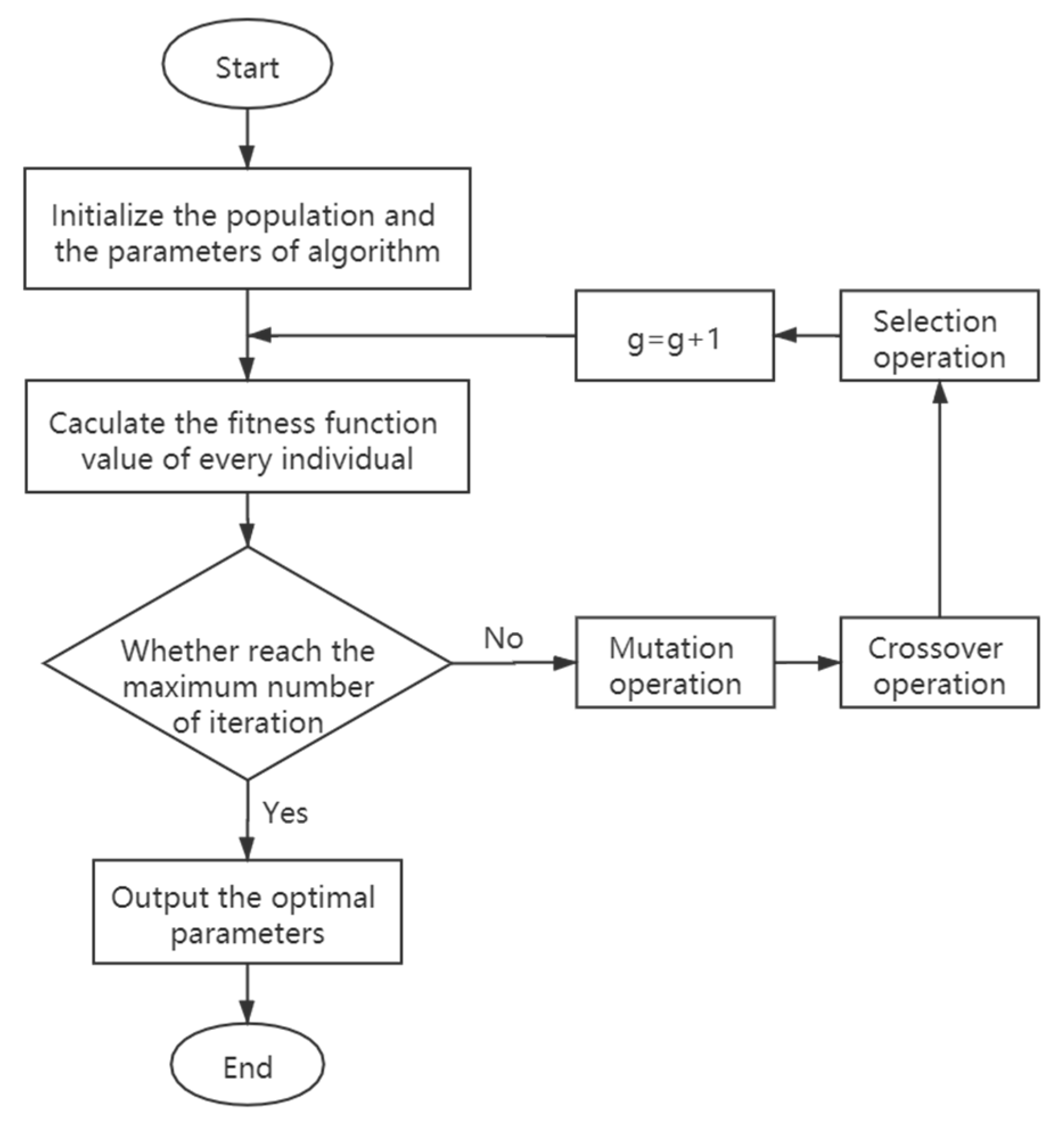
Step 6: Stop Test. Judge whether the termination condition is reached or the maximum evolutionary algebra is reached. If so, the evolution is terminated, and the optimal parameters obtained at this time are output as the solution. Otherwise, the program will jump to Step 2 for re-execution.
In order to reduce the number of hidden layer neurons and improve the generalization performance of the neural network, the global optimization capability of the DE algorithm is applied to the reasonable selection of the input weights and the hidden layer biases of the ELM.
Figure 7 shows the algorithm flow of the DE-ELM. Then, the optimization problem to be solved is to perform
, where
is the fitness function. Suppose that the cost function (
) is root mean squared error (RMSE) [
46]:
The RMSE on the whole training dataset is used as the fitness function. In the following section, we will carry out experiments to compare the classification effect of ELM, DE-ELM and SVM on the fatigue driving dataset.
Remark 1: Before training, we need to determine the parameters of the DE algorithm and the corresponding parameter selection criteria is given as follows. (i) The population size refers to the number of individuals in the population. When the population is large, the entire population exhibits diversity, which makes a larger search space and greater possibility of searching for the optimal solution, but the convergence rate will be reduced. On the other hand, when the population is small, the convergence rate is fast, but sometimes the global optimal solution cannot be obtained. (ii) The scaling parameter is used to control the amplification of the differential variation, which plays a moderating role in the local search and global search of the algorithm. When has large value, differential variation will have big impact on the mutation individual seen from (25) resulting in large disturbances, which is beneficial to maintain population diversity and global search capabilities. However, the search efficiency will be lower and the accuracy of the global optimal solution obtained will be lower. Smaller value of may lead to loss of population diversity and the algorithm is prone to fall into a local optimum causing early convergence. (iii) Crossover probability can determine whether members in a population perform crossover operations, which has an important impact on population diversity.
5. Results
In the experiments, after many trials and comparisons, the following parameters for the DE algorithm were determined:
. The experimental results are listed in
Table 2. As seen from
Table 2, with the increase in the hidden layer nodes number, the training accuracy and the testing accuracy of both the ELM and the DE-ELM are well improved. For the DE-ELM, when the number of hidden layer nodes is 150, it has better performance than the ELM with 200 nodes, in terms of both the training accuracy and the testing accuracy. It can also be seen that the DE-ELM using fewer hidden layer nodes can achieve better classification results than the ELM with more hidden layer nodes. The DE-ELM not only reduces network complexity, but also achieves stronger generation ability. Moreover, when the number of hidden layer nodes increases to 150 and 200, the training and test accuracies of SVM cannot compete with those of ELM and DE-ELM.
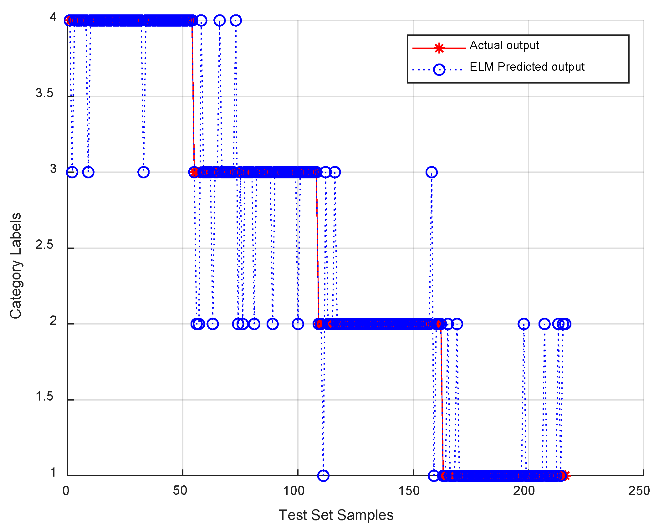
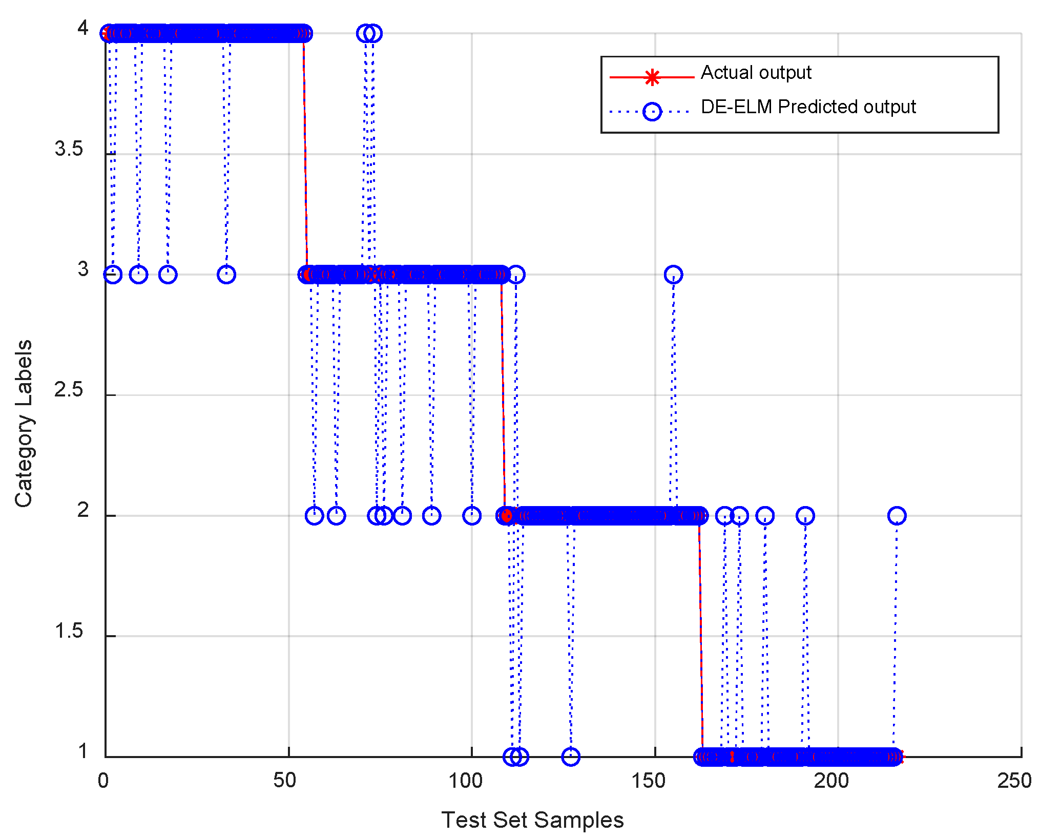
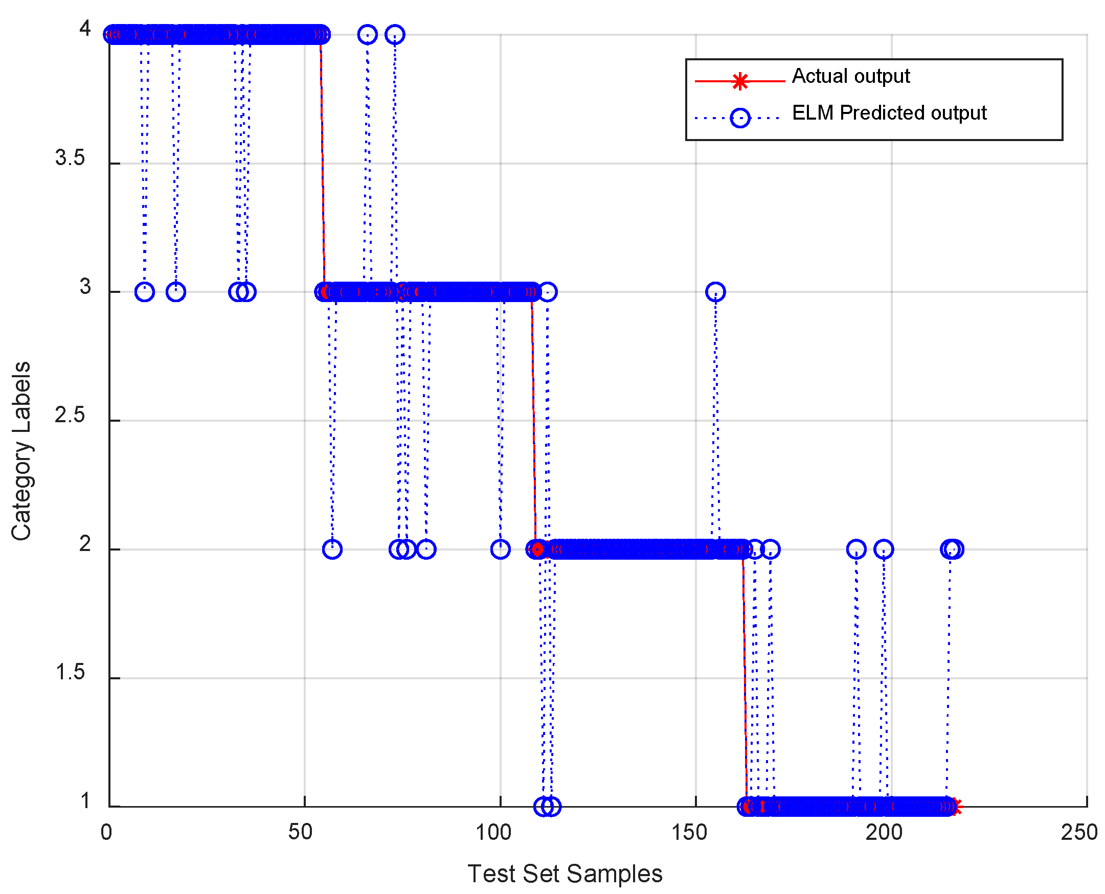
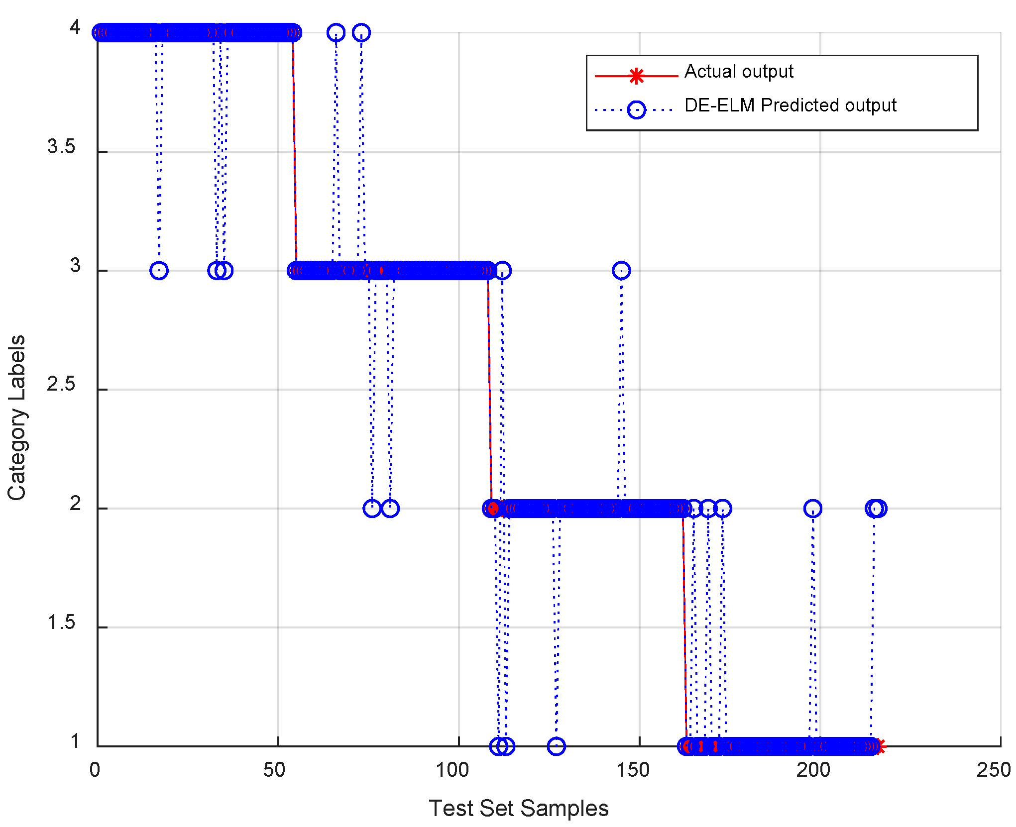
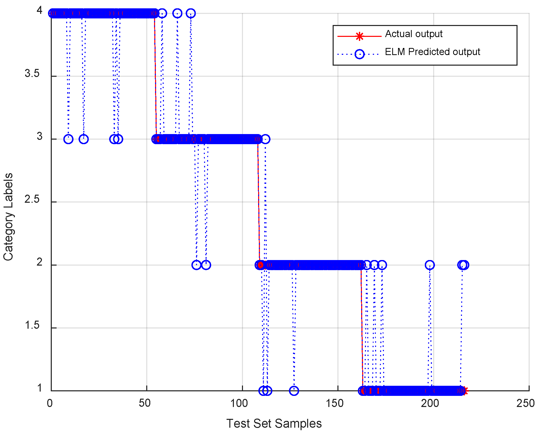
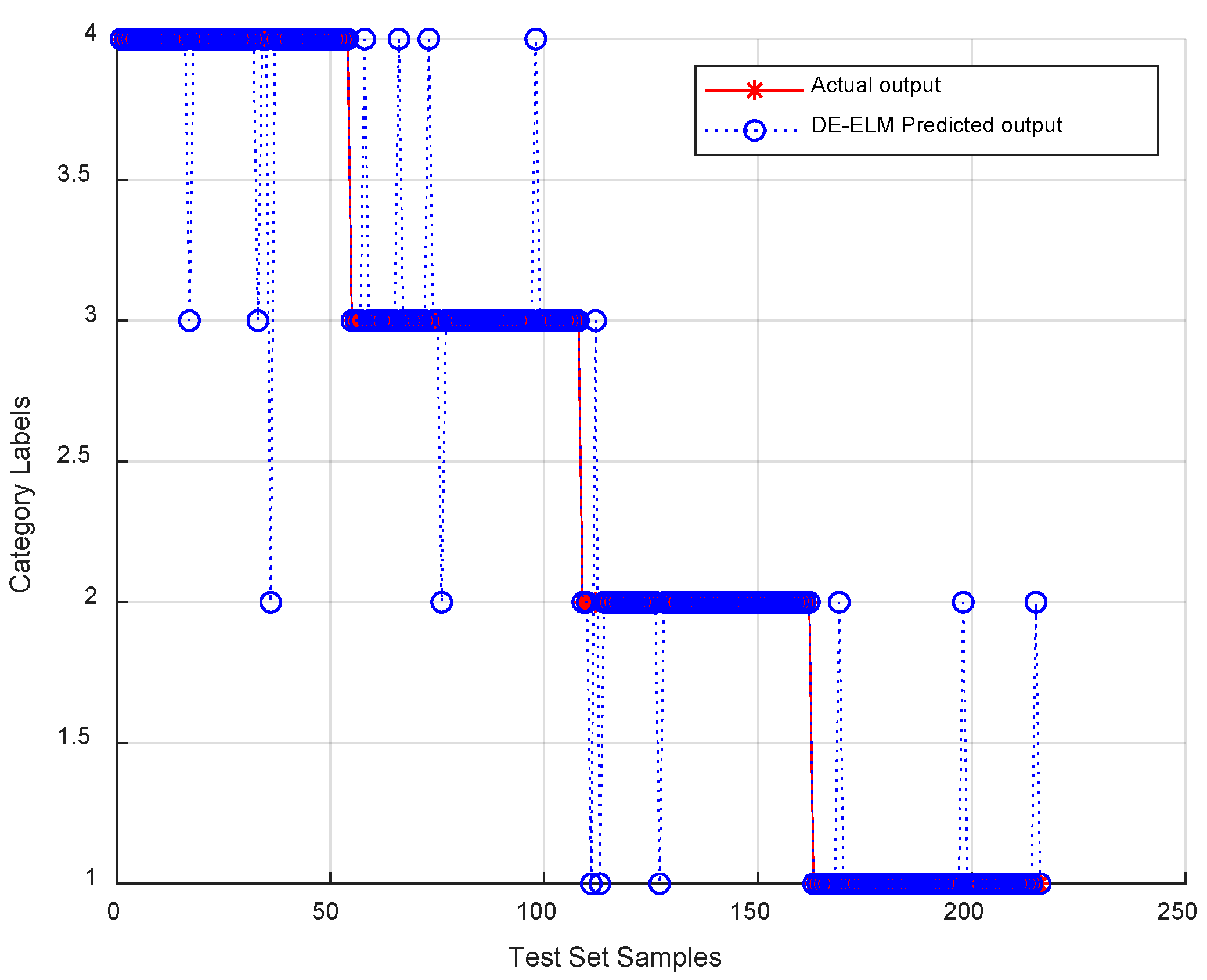
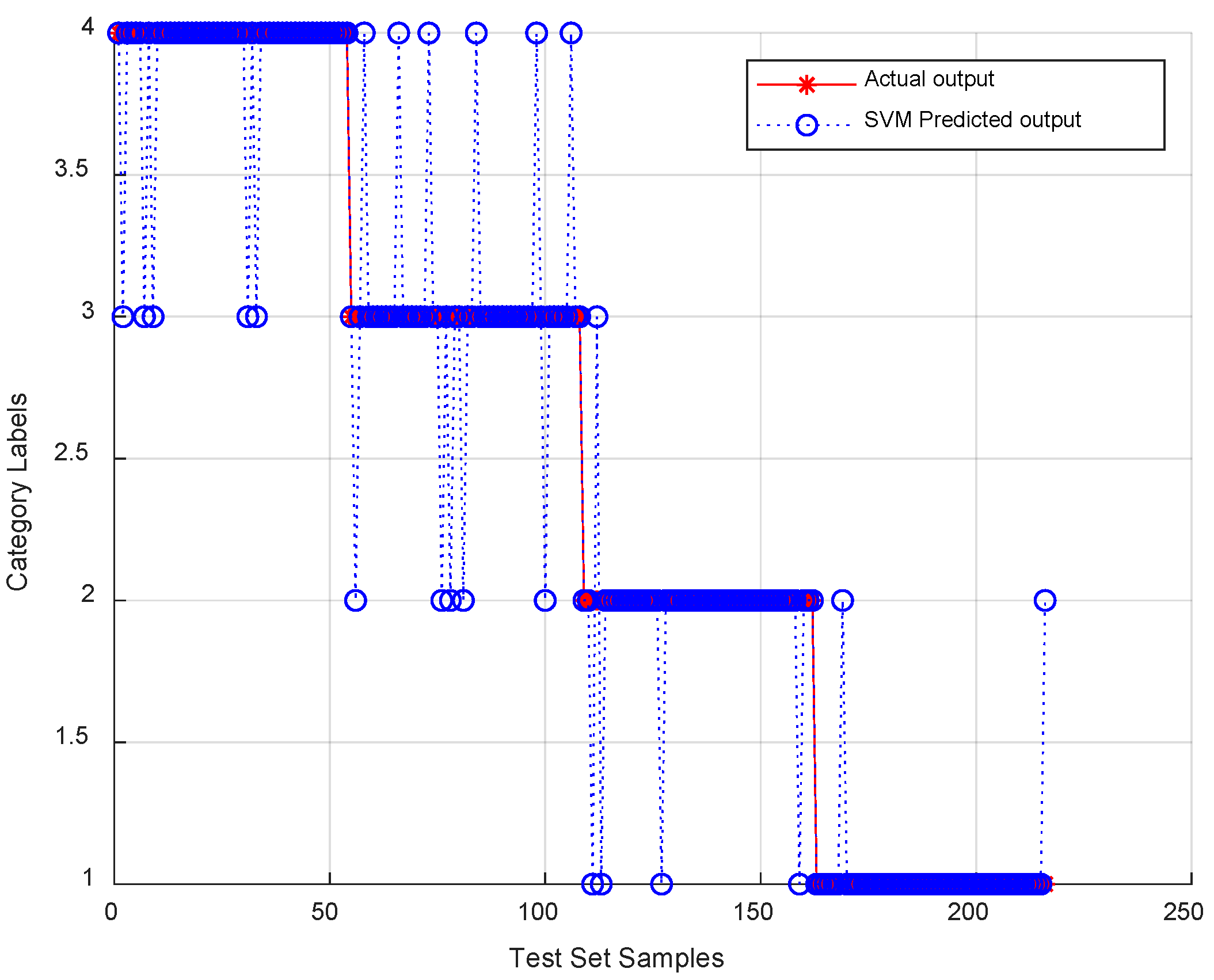
In order to further verify the effects of three approaches on the test set, the classification results on each fatigue state are shown in
Figure 8,
Figure 9,
Figure 10,
Figure 11,
Figure 12,
Figure 13 and
Figure 14, where the category labels of 1–4 represent the driver’s sober state, first-level fatigue state, second-level fatigue state and third-level fatigue state, respectively. The classification results of the ELM and the DE-ELM for 100, 150, and 200 hidden layer nodes are shown in
Figure 8,
Figure 9,
Figure 10,
Figure 11,
Figure 12 and
Figure 13, while the classification results of the SVM are shown in
Figure 14. It can be seen that, for the test set samples, the DE-ELM prediction outputs match with the actual outputs much better than the ELM and the SVM. In order to clearly evaluate the classification accuracy of the fatigue state,
Table 3 shows the classification accuracy of three approaches for each state on the test set when the number of hidden layer nodes is 200. It is worth noting that the recognition rate of the DE-ELM for various fatigue states all exceed 90%, which achieves the best classification performance. In detail, although the ELM obtains similar performance to the DE-ELM for the first and second level fatigue state, its classification accuracy for sober state and third-level fatigue state are not as good as DE-ELM. In addition, the classification accuracies of the DE-ELM are a lot better than the ones of the SVM for third-level fatigue states, except for the sober state in which similar accuracy is obtained. It clearly demonstrates that the developed DE-ELM method in this paper exhibits the most excellent classification performance of fatigue driving dataset compared to its ELM and SVM counterparts.
Please note that the criterion for determining the level of fatigue driving in this article is based on the evaluation method of facial video experts. This method only subjectively recognizes and judges the facial expression movement characteristics of the tester. It may not accurately and objectively determine the driver’s fatigue state, which also leads to a lower recognition rate of fatigue level in this experiment. The more input feature values and training samples of a classification model we have, the higher the classification accuracy we will obtain. Due to the limited conditions of this experiment, fewer input feature values and insufficient training samples have limited the recognition rate of fatigue level in this paper. Further studies on determining the fatigue level and the selection of input feature values will be carried out to obtain a higher recognition rate for fatigue driving.
