Modeling and Optimal Controller Based on Disturbance Detector for the Stabilization of a Three-link Inverted Pendulum Mobile Robot

Abstract

This work presents the realization of a complicated stabilization problem for a three inverted pendulum links-based mobile robot. The actuators of the mobile robot are direct current motors that have tachometer couplings to measure both the position and speed of the wheels and links. Using direct measurements under load and analyzing the deceleration curve, the motor parameters are determined experimentally. A mathematical model of the robot is obtained via the Euler–Lagrange equations. Next, the nonlinear model is linearized and discretized. Based on this discrete LTI model, an optimal controller is designed. The states and disturbances are estimated using a robust detector. Both the controller and detector are implemented in the robot processor. Numerical simulations and experimental tests show a good performance of the controller despite the presence of disturbances.

1. Introduction

Inverted pendulum mobile robots are an excellent testbed for implementing different classical control strategies and advanced controllers. The most common are the inverted pendulum on a cart [1], the double inverted pendulum on a cart [2], the double inverted pendulum with an actuator at the first joint (Pendubot) [3], and the double inverted pendulum with an actuator only in the second joint (acrobot) [4].

The wide application of this type of mobile robots has attracted the interest of many researchers in automatic control and robotics. Some examples of these applications are the personal transportation systems [5], walking design for humanoid robots [6], robotic wheelchairs [7], and educational purposes [8,9,10]. From the point of view of automatic control theory, the inverted pendulum mobile robot presents a complex stabilization problem, since it has only two wheels as a supporting point. One of the first researchers to tackle the stabilization control problem of two degrees of freedom inverted pendulum mobile robot was Yamamoto [11], who proposed a mathematical model with one input and two outputs. In the work presented by S.W. Nawawi [12], a sliding mode controller was used to balance an inverted pendulum-type mobile robot, also with two degrees of freedom.

Concerning to recent advancements about this kind of robots, in [13], the modified DAYANI method supported by a five-layered back-propagation neural network is used for the path control of a two-wheeled self-balancing robot. Using this method, the robot is able to find the optimal path from the starting point to the target point in a short time without hitting obstacles. In [14], a fuzzy controller and a PID controller are optimized using the particle swarm optimization algorithm. Both controllers are used for the stabilization of an under-actuated mobile robot. The optimized fuzzy controller shows a better suppression of system oscillations and current peaks than the optimized PID controller. In [15], the problem of the stabilization of a two-wheeled self-balanced vehicle is solved by using a nonlinear $H_{\infty }$. Despite external disturbances, un-modeled dynamics and extreme initial conditions, the system is able to work satisfactorily. In [16], a nonlinear proportional-derivative and a sliding mode controller using two reaction wheels are designed and implemented for an inverted pendulum. Both controllers overcome the performance of a previously presented PID controller. In [17], a self-balancing two-wheeled robot with two manipulator arms is considered. This robot is able to pick up objects. A dual-loop fuzzy control system is proposed to control the movement, rotation, and reach the desired position while keeping the robot in balance. In [18], the most common approaches for the modeling and control of such kind of systems are studied. To solve the stabilization problem, different kinds of controllers such as PD, LQR, $H_{\infty }$, backstepping, non-linear control, feedback linearization, model-based control, and model-based disturbance rejection control are studied. For the case of wheeled inverted pendulum systems subject to disturbances, a disturbance observer as feedforward compensation is proposed. Likewise, the design of a robust adaptive controller for the stabilization and trajectory tracking of such systems is considered. This control can work satisfactorily despite un-modeled dynamics and parametric uncertainties. Finally, advanced approaches based on soft computing such as neural networks, least squares support vector machine, and fuzzy logic are discussed. The performance of all the aforementioned controllers is tested by numerical simulations. On the other hand, regarding the use of inverted pendulum-type systems in education, in [19], a cheap portable arduino-based self-balancing robot is used to implement different strategies of control. All the different stages in the design and implementation process such as modeling, parameter estimation, programming, etc., are considered. In [20], a low-tech self-balancing human transportation vehicle is presented as a pedagogical tool for teaching feedback control concepts.

In this work, we have designed and assembled a mobile robot with five degrees of freedom and four inputs. It is a mobile robot whose supporting point is on its two wheels and whose links are three inverted pendulums. We have also done a complete theoretical analysis with sufficient mathematical foundations of the relationship between control systems and robotics. For the stabilization under disturbance of our mobile robot, we have designed an optimal controller based on two fundamental structural concepts for the compensation of dynamic systems: observability and controllability.

This article is organized as follows: Section 2 describes the development of the dynamic model of the mobile robot. Section 3 describes the design and assembly of the mobile robot, as well as its electronic characteristics. Section 4 presents the values of the parameters acquired from each motor of the mobile robot and the real-time response of each motor. In Section 5, we describe the mathematical model of the control law for the optimal stabilization for disturbed systems, while in Section 6, we synthesized, from an observer of state variables, a robust detector to estimate state variables and disturbances. In Section 7, we present the development of the optimal controller based on a robust detector for the stabilization of the mobile robot, and the closed-loop system diagram and numerical simulations that indicate a good performance of the controller. In Section 8, we can see the description and results of the implementation of the robust controller in the mobile robot, the movement of the wheels, and the stabilization of the mobile robot. Section 9 is dedicated to the discussion and conclusions about the results and experience obtained in this work. In Appendix A the general description of a discrete-time state-space model has been placed. Appendix B shows the matrices of the mobile robot’s non-linear model, while Appendix C contains the numerical matrices of the mobile robot, and finally Appendix D shows the efficient performance of the optimal controller based on the disturbance detector versus PD controller.

2. Dynamic Model of the Mobile Robot

Figure 1 shows the free-body diagram of the inverted pendulum mobile robot with five degrees of freedom. The masses of the links are defined as $m_1$, $m_2$, and $m_3$, and the mass of the wheel as $m_w$. It is assumed that the center of gravity coincides with the geometric center of the links that are at a distance of $l_1$, $l_2$, and $l_3$ ($l_i$ is the distance from joint i to the center of mass of the $i-th$ link, $i=1,\cdots ,3$). The angle of link 1 relative to the vertical is defined as ${\theta }_1$, the angle of link 2 relative to link 1 as ${\theta }_2$ and the angle of link 3 relative to link2 as ${\theta }_3$. Four torques act on the robot, ${\tau }_1,$ ${\tau }_2,$ ${\tau }_3$, and ${\tau }_4$, has five degrees of freedom ${\delta }_r,$ ${\delta }_l,$ ${\theta }_1,$ ${\theta }_2$, and ${\theta }_3$.

The mobile robot parameters are defined in

Table 1. Mobile robot parameters.

Parameter	Description	Value
$l_1$	Length to CG of link 1	10 cm
$l_2$	Length to CG of link 2	7.5 cm
$l_3$	Length to CG of link 3	5 cm
$m_1$	Mass of link 1	663 g
$m_2$	Mass of link 2	290 g
$m_3$	Mass of link 3	205 g
$m_w$	Mass of the wheel	53 g
$R_w$	Radius of the wheel	3.4 cm
H	Distance between the wheels	25.5 cm
$J_1$	Moment of inertia around the CM of link 1	22,100 gcm${}^2$
$J_2$	Moment of inertia around the CM of link 2	5437.5 gcm${}^2$
$J_3$	Moment of inertia around the CM of link 3	1708.3 gcm${}^2$
$J_w$	Moment of inertia of the wheel	306.34 gcm${}^2$

. The links are considered as uniform rods of mass M and length l. The moment of a rod’s inertia calculated about an axis of rotation, which is perpendicular to the rod and touches one end of the rod, is $J=\frac{1}{3}M{l}^2$. The wheels are considered as uniform discs of mass M y radius R. The moment of inertia of a uniform disc about an axis through its center is given by $J=\frac{1}{2}M{R}^2$.

The mobile robot’s mathematical model is obtained from the equations of Euler–Lagrange. The Euler–Lagrange equation is defined as [21]:

$$\frac{d}{dt}\left(\frac{\partial \Lambda }{\partial {\dot{q}}_i}\right)-\frac{\partial \Lambda }{\partial q_i}={\tau }_i,i=1,...;n$$

(1)

where ${\tau }_i$ is the vector of generalized forces, $q_i$ is the vector of generalized coordinates, ${\dot{q}}_i$ is the vector of joint velocities, $\Lambda =T-V$ is the Lagrangian, T is the kinetic energy of the system, and V is the potential energy of the system.

Equation (1) can be written in its compact form:

$$\tau =M\left(q\right)\ddot{q}+V(q,\dot{q})q+G\left(q\right)$$

(2)

where $M\left(q\right)$ is the inertia matrix, $V(q,\dot{q})$ is the Coriolis and centrifugal matrix, $g\left(q\right)$ is the vector of gravitational forces, q is the position vector, and $\dot{q}$ is the velocity vector.

The appropriate state variables to describe the dynamic model of the robot are the position q and the velocity $\dot{q}$. Then Equation (2) can be expressed in terms of the state vector: ${\left(\begin{array}{cc}q& \dot{q}\end{array}\right)}^T$ as:

$$\frac{d}{dt}\left(\begin{array}{c}q\\ \dot{q}\end{array}\right)=\left(\begin{array}{c}\dot{q}\\ M^{-1}\left(q\right)\left[\tau -V(q,\dot{q})q-G\left(q\right)\right]\end{array}\right);\left(\begin{array}{c}q\left(0\right)\\ \dot{q}\left(0\right)\end{array}\right)\in {\Re }^2$$

(3)

From the free body diagram of the robot (see Figure 1) it is determined that the generalized coordinate vector of the mobile robot is $q={\left(\begin{array}{ccccc}{q}_1& q_2& q_3& q_4& q_5\end{array}\right)}^T$, where $q_1={\delta }_r$, $q_2={\delta }_l$, $q_3={\theta }_1$, $q_4={\theta }_2$, $q_5={\theta }_3$.

The displacement of the right wheel is ${\delta }_r$, and ${\delta }_l$ is the displacement of the left wheel, and ${\theta }_1$, ${\theta }_2$, and ${\theta }_3$, are the angular position of the first, second, and third links respectively.

Denoting $\dot{q}$ and $\ddot{q}$ as $\dot{q}={\left(\begin{array}{ccccc}\dot{{\delta }_r}& \dot{{\delta }_r}& \dot{{\theta }_1}& \dot{{\theta }_2}& \dot{{\theta }_3}\end{array}\right)}^T$; $\ddot{q}={\left(\begin{array}{ccccc}\ddot{{\delta }_r}& \ddot{{\delta }_r}& \ddot{{\theta }_1}& \ddot{{\theta }_2}& \ddot{{\theta }_3}\end{array}\right)}^T$.

The kinetic and potential energy of the system are calculated. The robot model represented by the Euler–Lagrange equations is obtained:

$$\begin{array}{ccc}{M}_1{\ddot{\delta }}_r+M_2{\ddot{\delta }}_l+M_3{\ddot{\theta }}_1+M_4{\ddot{\theta }}_2+M_5{\ddot{\theta }}_3+V_1+G_1& =& {\tau }_1\\ M_2{\ddot{\delta }}_r+M_1{\ddot{\delta }}_l+M_3{\ddot{\theta }}_1+M_4{\ddot{\theta }}_2+M_5{\ddot{\theta }}_3+V_2+G_2& =& {\tau }_2\\ M_3{\ddot{\delta }}_r+M_3{\ddot{\delta }}_l+M_6{\ddot{\theta }}_1+M_7{\ddot{\theta }}_2+M_8{\ddot{\theta }}_3+V_3+G_3& =& 0\\ M_4{\ddot{\delta }}_r+M_4{\ddot{\delta }}_l+M_7{\ddot{\theta }}_1+M_9{\ddot{\theta }}_2+M_{10}{\ddot{\theta }}_3+V_4+G_4& =& {\tau }_3\\ M_5{\ddot{\delta }}_r+M_5{\ddot{\delta }}_l+M_8{\ddot{\theta }}_1+M_{10}{\ddot{\theta }}_2+M_{11}{\ddot{\theta }}_3+V_5+G_5& =& {\tau }_4\end{array}$$

(4)

In Appendix A, we can see the matrix representation of the system (4), where the matrix $M\left(q\right)$ $\in {\mathbb{R}}^{5\times 5}$ is the positive symmetric and definite inertia matrix, $V(q,\dot{q})q$ $\in {\mathbb{R}}^5$ contains the terms of centripetal and Coriolis forces, $G\left(q\right)$ $\in {\mathbb{R}}^5$ is the vector of gravitational forces, and the vector of applied pairs $\tau ={\left(\begin{array}{ccccc}{\tau }_1& {\tau }_2& 0& {\tau }_3& {\tau }_4\end{array}\right)}^T$ is produced by two actuators on the wheels, an actuator in the second link, and an actuator in the third link.

3. Design and Assembly of the Mobile Robot with Five Degrees of Freedom

For the construction of the mobile robot, five pieces were designed using SolidWorks software and manufactured in a 3D printer with PLA material, 5 Lego motors EV3 and two wheels of $3.4$ cm radius each were used (see Figure 2). A motor with a tachometer is coupled to each wheel. The accuracy of the tachometer is one degree [22]. The maximum speed of each motor is 160–170 RPM with 20 Ncm torque. In the third and fourth joints, two motors with the same characteristics are coupled, and in the fifth joint a motor with a maximum speed of 240–250 RPM with 8 Ncm torque is coupled. The robot has a rotation sensor EV3 implemented to measure the angular position of the first link with respect to the vertical axis. This is an EV3 gyroscopic sensor with an accuracy of $\pm 3$ degrees and a sample rate of 1 KHz. For the control of the mobile robot, a 300 MHz ARM9 Lego EV3 processor with a Linux-based operating system and a 64 MB RAM memory was acquired, which makes it suitable for the implementation of the optimal control law designed for the stabilization of the mobile robot. The power source is a lithium-ion EV3 rechargeable DC battery with a capacity of 2200 mAh. Communication with the computer and robot is via Wi-Fi.

4. Motors Control of the Mobile Robot

The motor parameters are shown in

Table 2. Motor parameters.

	$\mathit{\beta }$	${\mathit{K}}_{\mathit{e}}$	${\mathit{K}}_{\mathit{m}}$	${\mathit{R}}_{\mathit{a}}$	${\mathit{J}}_{\mathit{m}}$	$\mathit{G}\left(\mathit{s}\right)$
Motor 1	$0.000486$	$0.43798$	$0.27063$	$8.34$	$0.00101$	${\displaystyle \frac{2.207}{0.0688\mathrm{s}+1}}$
Motor 2	$0.000577$	$0.35732$	$0.24105$	$9.01$	$0.00125$	${\displaystyle \frac{2.639}{0.1235\mathrm{s}+1}}$
Motor 3	$0.000458$	$0.44706$	$0.31059$	$8.74$	$0.00123$	${\displaystyle \frac{2.174}{0.0755\mathrm{s}+1}}$
Motor 4	$0.000662$	$0.44535$	$0.30670$	$8.47$	$0.00118$	${\displaystyle \frac{2.1563}{0.0707\mathrm{s}+1}}$
Motor 5	$0.000206$	$0.27480$	$0.17340$	$12.22$	$0.00011$	${\displaystyle \frac{3.45}{0.028\mathrm{s}+1}}$

. These were obtained experimentally by direct measurements under load and analyzing the deceleration curve. The parameters $\beta$, $K_m$, $K_e$, $R_a$, and $J_m$ are the viscous friction coefficient, torque constant, back electromotive force constant, resistance, and moment of inertia of the motor, respectively. The transfer function that relates the voltage $V\left(s\right)$ to the angular velocity $\Omega \left(s\right)$ of a $DC$ motor is:

$$\begin{array}{ccccc}G\left(s\right)={\displaystyle \frac{V\left(s\right)}{\Omega \left(s\right)}}={\displaystyle \frac{\phi }{\alpha s+1}};\hfill & with& \phi ={\displaystyle \frac{K_m}{R_a\beta +K_e{K}_m}}& & \alpha ={\displaystyle \frac{R_a{J}_m}{R_a\beta +K_e{K}_m}}\end{array}$$

The real-time response for each motor is obtained by running the motor at full power and recording its angular velocity. Next, it is compared with the response of the system $G_i\left(s\right)$ obtained from the estimated parameters, as shown in Figure 3. Observing that the responses have the same behavior, validating the parameters obtained.

Torque Equation

Starting from the equation of the electrical subsystem of a DC motor:

$$u=Ri+L_a\frac{d}{dt}i+u_e$$

(5)

where R and $L_a$ represent the resistance and inductance of the motor, u represents the input voltage, and $u_e$ the back electromotive force (back EMF).

The torque equation is obtained in terms of the voltage input and motor speed:

$$\tau =\frac{K_m}{R}u-\frac{K_m{K}_e}{R}\dot{\theta }.$$

(6)

Using Equation (6) the torques of the mobile robot are determined, obtaining:

$$\tau =\left(\begin{array}{c}{\tau }_1\\ {\tau }_2\\ 0\\ {\tau }_3\\ {\tau }_4\end{array}\right)=\left(\begin{array}{c}\frac{K_{mr}}{R_r}{u}_1-\frac{K_{mr}{K}_{er}}{R_r{R}_w}{\dot{\delta }}_r\\ \frac{K_{ml}}{R_l}{u}_2-\frac{K_{ml}{K}_{el}}{R_l{R}_w}{\dot{\delta }}_l\\ 0\\ \frac{K_{m1}}{R_1}{u}_3-\frac{K_{m1}{K}_{e1}}{R_1}{\dot{\theta }}_2\\ \frac{K_{m2}}{R_2}{u}_4-\frac{K_{m2}{K}_{e2}}{R_2}{\dot{\theta }}_3\end{array}\right).$$

(7)

5. Optimal Stabilization

5.1. State Variables Model of Mobile Robot

Let the vector of states $x={\left(\begin{array}{cc}{x}_1& x_2\end{array}\right)}^T$ such that $x_1=q$; $x_2=\dot{q}$. According to the Equation (3) we get:

$$\begin{array}{ccc}\hfill {\dot{x}}_1& =& \dot{q}=x_2\hfill \\ \hfill {\dot{x}}_2& =& \ddot{q}=M^{-1}\left(x_1\right)\left[u-V(x_1,x_2)x_2-G\left(x_1\right)\right]\hfill \end{array}$$

where $x_1={\left(\begin{array}{ccccc}{\delta }_r& {\delta }_l& {\theta }_1& {\theta }_2& {\theta }_3\end{array}\right)}^T;$ $x_2={\left(\begin{array}{ccccc}{\dot{\delta }}_r& {\dot{\delta }}_l& {\dot{\theta }}_1& {\dot{\theta }}_2& {\dot{\theta }}_3\end{array}\right)}^T$. Linearizing the system around the operating point ${\delta }_r=$ ${\delta }_l={\theta }_1={\theta }_2={\theta }_3={\dot{\delta }}_r={\dot{\delta }}_l={\dot{\theta }}_1={\dot{\theta }}_2={\dot{\theta }}_3=0$ and $u_1=u_2=u_3=u_4=0$ and discretizing the system with a sampling period of $t_s=0.005s$, the numerical matrices A y B of the mobile robot are obtained (see these matrices in Appendix C).

The eigenvalues of matrix A are: $\{1.0;1.0;0.3837;0.7916;0.859;0.926;0.972;1.03;1.05;1.055\}$. Since not all eigenvalues are within the unit circle, the system is unstable.

5.2. Optimal Control for Systems with Disturbances

The objective is to find an optimal control law $u_k$ that minimizes the performance index $J_i$ in the interval $[k,N]$. The performance index is given by [23,24,25]:

$$J_i=\frac{1}{2}{x}_N^T{Q}_f{x}_N+\frac{1}{2}\sum _{k=1}^{N-1}\left[x_k^{T}Q{x}_k+u_k^{T}R{u}_k\right]$$

where Q is a positive definite symmetric matrix (or positive semi-defined), R is a positive definite symmetric matrix, and $Q_f$ is a positive definite (or positive semi-defined) symmetric matrix.

The term $u_k^{T}R{u}_k$ is related to the energy expenditure of the $u_k$ control, the term $x_k^{T}Q{x}_k$ is related to the intermediate states, and the term $x_N^T{Q}_f{x}_N$ is related to the final states.

The control law has the form:

$$u_k=-K_k{x}_k+K_k^v{h}_{k+1}$$

where $K_k$ is the feedback gain matrix, $K_k^v$ is the gain matrix that depends on the disturbance input $w_k$, and $h_{k+1}$ is obtained by solving the differential equation:

$$h_k={\left(A-B{K}_k\right)}^T{h}_{k+1}+P_{k+1}E{w}_k$$

with

$$h_N=0$$

and

$$\begin{array}{ccc}\hfill K_k& =& {\left(B^T{P}_{k+1}B-R\right)}^{-1}{B}^T{P}_{k+1}A\hfill \\ \hfill K_k^v& =& {\left(B^T{P}_{k+1}B-R\right)}^{-1}{B}^T\hfill \end{array}$$

where $P_{k+1}$ is the positive symmetric and definite solution matrix of the Riccati equation.

$$P_k=A^T{P}_{k+1}\left(A-B{K}_k\right)+C^{T}QC$$

with

$$P_N=C^T{Q}_{f}C.$$

6. Robust Detector for Systems with Disturbances

The equations for the linear system with disturbance $w_k$ are:

$$\begin{array}{ccc}\hfill x_{k+1}& =& A{x}_k+B{u}_k+E{w}_k\hfill \end{array}$$

(8)

$$\begin{array}{ccc}\hfill y_k& =& C{x}_k.\hfill \end{array}$$

(9)

Considering the state observer:

$${\tilde{x}}_{k+1}=\left(A-\varphi C\right){\tilde{x}}_k+B{u}_k+\varphi y_k$$

(10)

where $\varphi$ is the gain matrix of the observer. Let $e_k={\tilde{x}}_k-x_k$, then the error dynamics of the system is:

$$e_{k+1}=\left(A-\varphi C\right)e_k-E{w}_k.$$

(11)

In Equation (11), it can be observed that even when the eigenvalues of the matrix $(A-\varphi C)$ are stable, the presence of the disturbance $w_k$ does not guarantee that ${lim}_{k\to \infty }{e}_{k+1}$ tends to zero, so that from the observer (10) we proceed to synthesize a robust detector of disturbance that guarantees the zero convergence of the error $e_{k+1}$.

Synthesis of a Robust Detector for Disturbances

For the synthesis [26] of a disturbance detector, a new output built as $Y=\left(\begin{array}{c}{y}_k\\ y_{k+1}\end{array}\right)$. As $y_k=C{x}_k,$ then $y_{k+1}=C{x}_{k+1}=CA{x}_k+CB{u}_k+CE{w}_k$. Therefore, the new output Y has the form:

$$Y=\left(\begin{array}{c}C\\ CA\end{array}\right)x_k+\left(\begin{array}{c}0\\ CB\end{array}\right)u_k+\left(\begin{array}{c}0\\ CE\end{array}\right)w_k$$

Let,

$$\tilde{Y}=\left(\begin{array}{c}{\tilde{y}}_k\\ {\tilde{y}}_{k+1}\end{array}\right).$$

Then the expression $C{x}_{k+1}$ has the form:

$$C{x}_{k+1}=C\left[\left(A-LC\right){\tilde{x}}_k+Ly+B{u}_k\right]$$

where L is the gain matrix of the disturbance detector. Performing the corresponding calculations, we obtain that:

$$C_{k+1}=CA{\tilde{x}}_k+CB{u}_k$$

where

$$\tilde{Y}=\left(\begin{array}{c}C\\ CA\end{array}\right){\tilde{x}}_k+\left(\begin{array}{c}0\\ CB\end{array}\right)u_k.$$

The detector for the disturbed system is defined by the dynamics:

$${\tilde{x}}_{k+1}=A{\tilde{x}}_k+B{u}_k+L(Y-\tilde{Y}).$$

The dynamics of the detection error has the form:

$$e_{k+1}=\left[A-L\left(\begin{array}{c}C\\ CA\end{array}\right)\right]e_k+\left[L\left(\begin{array}{c}0\\ CE\end{array}\right)-E\right]w_k.$$

Let $L=(L_1\hspace{1em}{L}_2)$ and by rewriting, we have:

$$e_{k+1}=\left[\overline{A}-L_{1}C\right]e_k+\left[\left(L_{2}C-I\right)E\right]w_k$$

where

$$\overline{A}=\left(I-L_{2}C\right)A.$$

Then, if the pair $(\overline{A},C)$ is detectable, a matrix $L_1$ can be found such that the matrix $\left(\overline{A}-L_{1}C\right)$ is asymptotically stable. To avoid the effect of disturbances on the estimation error, an $L_2$ matrix must be found such that:

$$E\in Ker\left(L_{2}C-I\right).$$

7. Optimal Control Design Based on a Disturbance Detector to Stabilize the Mobile Robot

In order to stabilize the mobile robot around the equilibrium point, an optimal controller based on a disturbance detector is designed.

Using the controllability and observability matrices, it is verified that the mobile robot is a fully controllable and observable system:

$$\begin{array}{ccc}\hfill M_c& =& \left(\begin{array}{ccccc}B& AB& A^{2}B& \cdots & A^{9}B\end{array}\right),rank\left(M_c\right)=10\hfill \\ \hfill M_o& =& {\left(\begin{array}{ccccc}C& CA& C{A}^2& \cdots & C{A}^9\end{array}\right)}^T,rank\left(M_o\right)=10.\hfill \end{array}$$

Appendix C shows the numerical gain matrix $L=\left(\begin{array}{cc}{L}_1& L_2\end{array}\right)$ of the robust detector, such that $(L_{2}C-I)E=0$ and $\left(\overline{A}-L_{1}C\right)$ is asymptotically stable, with eigenvalues: $\{0.1999$ multiplicity 5; 0.1997 multiplicity $5\}$. Subsequently, the matrices A and B of the robot system are replaced in the Riccati equation and finding the positive defined symmetric solution, the numerical feedback matrix $K_k$ (see Appendix C) that stabilizes the system is obtained. Let:

$$\begin{array}{ccc}\hfill Q& =& diag\left(\begin{array}{cccccccccc}20& 20& 1\times {10}^7& 1& 1& 1& 1& 1& 1& 1\end{array}\right)\hfill \\ \hfill R& =& diag\left(\begin{array}{ccccc}50& 50& 50& 5000& 5000\end{array}\right).\hfill \end{array}$$

The weight matrices Q and R were selected by observing the behavior of the system in numerical simulations. A higher weighting factor was given to the stabilization of the pendulum angle on the vertical axis. The goal is to obtain a fast stabilization process without reaching the input saturation of the motors.

Simulations

The Matlab-Simulink software was used to verify the performance of the controller, according to the diagram in Figure 4, with a simulation time of 4 s, implementing a disturbance $w_k$ that adds to the control signal $u_1$ and $u_2$ in 1 Volt during the period of $1.5$ s to 2 s, under the initial conditions:

$$\begin{array}{ccc}\hfill x\left(0\right)& =& {\left(\begin{array}{cccccccccc}2& 2& 0.1& 0.1& 0.1& 0& 0& 0& 0& 0\end{array}\right)}^T\hfill \\ \hfill \tilde{x}\left(0\right)& =& {\left(\begin{array}{cccccccccc}1& 1& 0.05& 0.05& 0.05& 1& 1& 1& 1& 1\end{array}\right)}^T\hfill \end{array}$$

Figure 5 shows the tracking of the original states with the estimated states even when disturbances occur at $t=1.5$ s and $t=2$ s. For this reason, estimation errors (differences between estimated state and original state) tend to zero. See Figure 6.

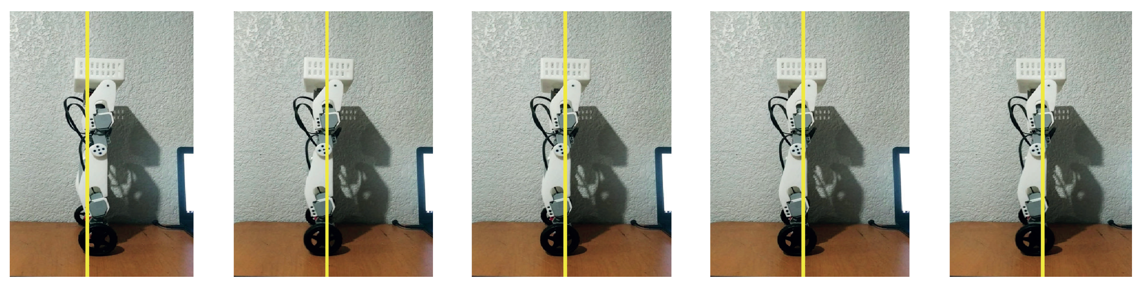
8. Real-Time Experimentation

Using the Matlab Simulink platform, the optimal detector-based control is implemented using the feedback gains calculated above. By using the Simulink Lego mindstorms EV3 library it is possible to access the sensors and generate the robot states from them, calculate the control input, and implement it to the motors. The position and speed signals obtained by the encoder and gyroscope, respectively, are conveniently conditioned using a low pass filter. The driver implementation is performed for a period of 50 s, using the diagram in Figure 7.

As well as the disturbance:

$$w_k=\left\{\begin{array}{cc}{\left(\begin{array}{ccccc}0& 0& 0& 0& 0\end{array}\right)}^T& k{t}_s<20\\ {\left(\begin{array}{ccccc}1& 1& 0& 0& 0\end{array}\right)}^T& 20\le k{t}_s\le 30\\ {\left(\begin{array}{ccccc}0& 0& 0& 0& 0\end{array}\right)}^T& 30<k{t}_s\end{array}\right.$$

In Figure 8, Figure 9 and Figure 10, the red graphics represent the numerical simulations and the blue graphics represent real-time experiments.

Figure 8a,b show the behavior of the displacement of the right wheel and left wheel of the mobile robot, taking maximum values of 3 and −2.5 cm during the first 50 s of the experiment. Figure 8c shows the behavior of the tilt angle of link 1 of the mobile robot, which takes values of $-0.34$ and 0.017 radians the first 50 s of the experiment. The responses of the tilt angle of links 2 and 3 respectively, having maximum values of −0.05 and 0.05 radians are presented in Figure 8d,e.

Figure 9a,b show the velocity of the left wheel and right wheel taking values between $-10$ and 10 cm/s. Figure 9c–e present the angular velocity of links 1, 2, and 3 with ranges $[-0.3,0.2]$ rad/s, $[-0.4,0.4]$ rad/s, and $[-0.05,0.04]$ rad/s, respectively.

In Figure 10a,b the control inputs to the right and left wheel motor are shown. In Figure 10c,d the control inputs of the second and third link motors are presented, having values between $[-2.5,1]$ V and $\pm 1$ V. It is important to mention that, as can be verified, the control signals for the motors are within the operating range $\pm 7.6$ V. That is, there is no saturation.

The differences between simulated and experimental responses may be mainly due to un-modeled dynamics, sensor, and actuator noises. Nonetheless, in general, as can be appreciated, such differences are not significant for the achievement of the main goal of the controller, that is, to keep the system in balance. In fact, from Figure 10, it is interesting to observe the ability of the control signal to compensate for the deleterious effect of noises, disturbances, and un-modeled dynamics. Thus, it can be considered that the experimental performance of the controller is good, particularly considering the difficulty of the stabilization problem.

Figure 11 shows the robot’s behavior during the experiment, maintaining a tilt angle close to zero with respect to the vertical axis and remaining at the same point with respect to the horizontal axis throughout the time of the experiment.

Appendix D describes the comparison with another control technique known as PD (Proportional-Derivative).

9. Conclusions

The proposed inverted pendulum mobile robot is an excellent reference problem for studies of advanced control techniques, due to the complex task of keeping its structure in balance. We decided to develop an optimal disturbance detector-based controller for our mobile robot. The controller was implemented using the Matlab-Simulink algorithm via a Wi-Fi connection with the robot. Stabilization in the vertical position of the robot was successfully achieved. The oscillations that occurred when there were no disturbances were approximately $\pm 0.017$ rad, measured by the gyroscope coupled to the first link. When a slight force is applied contrary to the movement of the robot (disturbance), the oscillations that occurred were $\pm 0.035$ rad with $\pm 5$ V requirement for the two-wheel motors, while the behavior of links 2 and 3 presented values between $[0,0.5]$ rad and $[0,-0.05]$ rad with a requirement of $[1,-2.5]$ V and $\pm 1$ V.

For future work, an extension of the current controller will be used to cope with the tracking trajectory problem. Likewise, the Coefficient of Friction between the robot body and motors, as well as the Coefficient of Friction between the robot wheels and bearing surface will be studied. Besides, the uncertainty associated with some robot parameters, and a variable load in the last link could be considered. Finally, the problem of ascending and descending ramps will be addressed.

References

1. Gopikrishnan, S.; Kesarkar, A.A.; Selvaganesan, N. Design of fractional controller for cart-pendulum SIMO system. In Proceedings of the IEEE International Conference on Advanced Communication Control and Computing Technologies (ICACCCT), Ramanathapuram, India, 23–25 August 2012; pp. 170–174. [Google Scholar]
2. Inoue, A.; Deng, M.; Tanabe, T. Practical swing-up control system design of cart-type double inverted pendulum. In Proceedings of the IEEE Chinese Control Conference, Harbin, China, 7–11 August 2006; pp. 2141–2146. [Google Scholar]
3. Eom, M.; Chwa, D. Robust swing-up and balancing control using a nonlinear disturbance observer for the pendubot system with dynamic friction. IEEE Trans. Robot. 2015, 31, 331–343. [Google Scholar] [CrossRef]
4. Cao, J.-Q.; Lai, X.-Z.; Min, W. Position control method for a planar Acrobot based on fuzzy control. In Proceedings of the IEEE 34th Chinese Control Conference (CCC), Hangzhou, China, 28–30 July 2015; pp. 923–927. [Google Scholar]
5. Lee, H.J.; Kim, H.W.; Jung, S. Development of a mobile inverted pendulum robot system as a personal transportation vehicle with two driving modes: TransBOT. In Proceedings of the IEEE World Automation Congress, Kobe, Japan, 19–23 September 2010; pp. 1–5. [Google Scholar]
6. Mohamed, S.A.; Maged, S.A.; Awad, M.I. Design and Control of the Lower Part of Humanoid Biped Robot. In Proceedings of the IEEE 3rd International Conference on Robotics and Automation Engineering (ICRAE), Guangzhou, China, 17–19 November 2018; pp. 19–23. [Google Scholar]
7. Hamatani, S.; Murakami, T. A novel steering mechanism of two-wheeled wheel chair for stability improvement. In Proceedings of the IECON 2015-41st Annual Conference of the IEEE Industrial Electronics Society, Yokohama, Japan, 9–12 November 2015; pp. 2154–2159. [Google Scholar]
8. Solis, J.; Nakadate, R.; Yoshimura, Y.; Hama, Y.; Takanishi, A. Development of the two-wheeled inverted pendulum type mobile robot WV-2R for educational purposes. In Proceedings of the IEEE/RSJ International Conference on Intelligent Robots and Systems, St. Louis, MO, USA, 10–15 October 2009; pp. 2347–2352. [Google Scholar]
9. Reck, R.M.; Sreenivas, R.S. Developing an affordable and portable control systems laboratory kit with a Raspberry Pi. Electronics 2016, 5, 36. [Google Scholar] [CrossRef] [Green Version]
10. Ordóñez Cerezo, J.; Castillo Morales, E.; Cañas Plaza, J.M. Control system in open-source FPGA for a self-balancing robot. Electronics 2019, 8, 198. [Google Scholar] [CrossRef] [Green Version]
11. Yamamoto, Y. NXTway-GS Model-Based Design-Control of Self-Balancing Two-Wheeled Robot Built with LEGO Mindstorms NXT. Available online: https://la.mathworks.com/matlabcentral/fileexchange/19147-nxtway-gs-self-balancing-two-wheeled-robot-controller-design (accessed on 17 August 2020).
12. Nawawi, S.W.; Ahmad, M.N.; Osman, J.H.S. Control of two-wheels inverted pendulum mobile robot using full order sliding mode control. In Proceedings of the International Conference on Man-Machine Systems, Budapest, Hungary, 9–12 October 2006; pp. 15–16. [Google Scholar]
13. Chhotray, A.; Parhi, D. Navigational control analysis of two-wheeled self-balancing robot in an unknown terrain using back-propagation neural network integrated modified DAYANI approach. Robotica 2019, 37, 1346–1362. [Google Scholar] [CrossRef]
14. Odry, À.; Fullér, R. Comparison of optimized PID and fuzzy control strategies on a mobile pendulum robot. In Proceedings of the IEEE 12th International Symposium on Applied Computational Intelligence and Informatics (SACI), Timisoara, Romania, 17–19 May 2018; pp. 207–212. [Google Scholar]
15. Raffo, G.V.; Ortega, M.G.; Madero, V.; Rubio, F.R. Two-wheeled self-balanced pendulum workspace improvement via underactuated robust nonlinear control. Control. Eng. Pract. 2019, 44, 231–242. [Google Scholar] [CrossRef]
16. Trentin, J.; Da Silva, S.; Ribeiro, J.M.D.S.; Schaub, H. Inverted Pendulum Nonlinear Controllers Using Two Reaction Wheels: Design and Implementation. IEEE Access 2020, 8, 74922–74932. [Google Scholar] [CrossRef]
17. Hsu, C.F.; Kao, W.F. Double-loop fuzzy motion control with CoG supervisor for two-wheeled self-balancing assistant robots. Int. J. Dyn. Control. 2020, 8, 851–866. [Google Scholar] [CrossRef]
18. Li, Z.; Yang, C.; Fan, L. Advanced Control of Wheeled Inverted Pendulum Systems; Springer Science and Business Media: Berlin/Heidelberg, Germany, 2012. [Google Scholar]
19. Odry, Á.; Fullér, R.; Rudas, I.J.; Odry, P. Fuzzy control of self-balancing robots: A control laboratory project. Comput. Appl. Eng. Educ. 2020, 28, 512–535. [Google Scholar] [CrossRef]
20. Lin, S.; Tsai, C. Development of a self-balancing human transportation vehicle for the teaching of feedback control. IEEE TRansactions Educ. 2008, 52, 157–168. [Google Scholar] [CrossRef]
21. Reyes, F. Robótica: Control de Robots Manipuladores; Alfaomega Grupo Editor: Mexico city, Mexico, 2011. [Google Scholar]
22. Garber, G. Learning LEGO Mindstorms EV3; Packt Publishing Ltd.: Birmingham, UK, 2015. [Google Scholar]
23. Fossen, T.I. Handbook of Marine Craft Hydrodynamics and Motion Control; John Wiley and Sons: Hoboken, NJ, USA, 2011. [Google Scholar]
24. Sinha, A. Linear Systems: Optimal and Robust Control; CRC Press: Boca Raton, FL, USA, 2007. [Google Scholar]
25. Kiumarsi-Khomartash, B.; Lewis, F.L.; Naghibi-Sistani, M.B.; Karimpour, A. Optimal tracking control for linear discrete-time systems using reinforcement learning. In Proceedings of the 52nd IEEE Conference on Decision and Control, Florence, Italy, 10–13 December 2013; pp. 3845–3850. [Google Scholar]
26. Ding, X. Steven Model-Based Fault Diagnosis Techniques; Springer: Berlin/Heidelberg, Germany, 2008; ISBN 9783540763031. [Google Scholar]
27. Ogata, K. Discrete-Time Control Systems; Prentice Hall: Englewood Cliffs, NJ, USA, 1995; Volume 2. [Google Scholar]
28. Kailath, T. Linear Systems; Prentice-Hall: Englewood Cliffs, NJ, USA, 1980; Volume 156. [Google Scholar]
29. Fortuna, L.; Frasca, M. Optimal and Robust Control: Advanced Topics with Matlab; CRC Press: Boca Raton, FL, USA, 2012. [Google Scholar]
30. Fadali, M.S.; Visioli, A. Digital Control Engineering: Analysis and Design; Academic Press: Cambridge, MA, USA, 2013. [Google Scholar]
Figure 1. Diagram of an underactuated mobile robot with five degrees of freedom.
Electronics 09 01821 g001
Figure 2. Assembly of the mobile robot.
Electronics 09 01821 g002
Figure 3. Motor real-time response.
Electronics 09 01821 g003
Figure 4. Implementation diagram.
Electronics 09 01821 g004
Figure 5. Response of original states vs. estimated states. (a) δ r vs. δ r ˜ ; (b) δ l vs. δ l ˜ ; (c) θ 1 vs. θ 1 ˜ ; (d) θ 2 vs. θ 2 ˜ ; (e) θ 3 vs. θ 3 ˜ ; (f) δ ˙ r vs. δ r ˜ ˙ ; (g) δ ˙ l vs. δ l ˜ ˙ ; (h) θ ˙ 1 vs. θ 1 ˜ ˙ ; (i) θ ˙ 2 vs. θ 2 ˜ ˙ ; and (j) θ ˙ 3 vs. θ 3 ˜ ˙ .
Electronics 09 01821 g005
Figure 6. Estimation errors.
Electronics 09 01821 g006
Figure 7. Real-time implementation diagram.
Electronics 09 01821 g007
Figure 8. Response of position states: (a) Displacement of the right wheel δ r , (b) displacement of the left wheel δ l , (c) tilt angle of the first link θ 1 , (d) tilt angle of the second link θ 2 , and (e) tilt angle of the third link θ 3 .
Electronics 09 01821 g008
Figure 9. Response of velocities states: (a) Linear velocity of the right wheel δ ˙ r , (b) linear velocity of the left wheel δ ˙ l , (c) angular velocity of the first link θ ˙ 1 , (d) angular velocity of the second link θ ˙ 2 , and (e) angular velocity of the third link θ ˙ 3 .
Electronics 09 01821 g009
Figure 10. Control inputs: (a) Control input u 1 for the right wheel motor, (b) control input u 2 for the left wheel motor, (c) control input u 3 for the second link motor and, (d) control input u 4 for the third link motor.
Electronics 09 01821 g010
Figure 11. Mobile robot stabilization.
Electronics 09 01821 g011