Underground Cylindrical Objects Detection and Diameter Identification in GPR B-Scans via the CNN-LSTM Framework

Abstract

Ground penetrating radar (GPR), as a non-invasive instrument, has been widely used in the civil field. The interpretation of GPR data plays a vital role in underground infrastructures to transfer raw data to the interested information, such as diameter. However, the diameter identification of objects in GPR B-scans is a tedious and labor-intensive task, which limits the further application in the field environment. The paper proposes a deep learning-based scheme to solve the issue. First, an adaptive target region detection (ATRD) algorithm is proposed to extract the regions from B-scans that contain hyperbolic signatures. Then, a Convolutional Neural Network-Long Short-Term Memory (CNN-LSTM) framework is developed that integrates Convolutional Neural Network (CNN) and Long Short-Term Memory (LSTM) network to extract hyperbola region features. It transfers the task of diameter identification into a task of hyperbola region classification. Experimental results conducted on both simulated and field datasets demonstrate that the proposed scheme has a promising performance for diameter identification. The CNN-LSTM framework achieves an accuracy of 99.5% on simulated datasets and 92.5% on field datasets.

1. Introduction

Ground-penetrating radar (GPR) is an important non-destructive evaluation (NDE) method [1,2]. Over the past decade, GPR has been widely applied to geological exploration [3], landmine detection [4], and NDE of structures [5]. In civil field, it has become a routine tool for inspecting rebars in concrete, locating subsurface utilities, structural evaluation, etc. [6,7,8,9]. It utilizes underground materials’ different electromagnetic properties to detect underground areas based on the propagation and scattering characteristics of high-frequency electromagnetic (EM) waves [10,11,12]. Scattering from a single point or cylinder, such as rebar and pipeline, will produce hyperbolic reflection characteristics in the recorded GPR B-scans [13,14]. As a result, the detection of the hyperbola regions in the GRP B-scans is equivalent to the detection of the underground targets. Thus, the problem of underground targets detection can be transferred to the detection of hyperbola regions.

In the process of civil infrastructure construction, more and more cylindrical objects are buried underground, including rebars, pipelines (gas, water, oil, sewage, etc.), cylindrical tanks, and cables (energy, optical, signal). It is particularly important to accurately estimate the diameter of cylindrical underground objects with GPR technology [15]. However, the diameter estimation of underground cylindrical objects from GPR B-scans often requires manual interaction [16]. The high time consumption limits its application in the field environment. Therefore, the researchers have aroused great interest in the automatic detection and interpretation of GPR data in recent years [17]. Interpretation of GPR B-scans usually consists of two parts: hyperbola region detection and parameter estimation (e.g., diameter).

The detection of hyperbola region from B-scans is a first step of GPR data interpretation, after that, the parameters estimation of underground cylindrical objects can be conducted based on the picked regions [18]. In Reference [19], the Hough transform was first used for hyperbola detection in GPR B-scans. It can transform the global curve detection problem into an effective peak detection problem in the Hough parameter space. The Viola-Jones algorithm has been used to narrow the range of the reflection hyperbola. A generalized Hough transform was used to detect the hyperbolas and to derive the hyperbolic parameters [20]. However, Hough transform is computationally expensive. In addition, some image processing methods are used to process radar signals [21,22]. An advanced imaging algorithm was proposed for automated detection of the hyperbola region, which used the Canny edge detector and performed well [21]. Extensive research has applied deep learning (DL) techniques to process radar signals [6,23,24,25]. In Reference [23], GPR waveform signals were classified by a neural network classifier to determine hyperbola regions. However, it is susceptible to clutter and noise. The work in Reference [24] designed a binary classifier which employed high-order statistic cumulant features and used a multi-objective genetic approach for hyperbola detection. In Reference [6], a method based on template matching and Convolutional Neural Network (CNN) was provided for hyperbola region detection. The matching template was designed to traverse GPR B-scans and the region with high similarity was calculated as the pre-detection region. Then, the CNN was used to eliminate the non-hyperbolic region and obtain the hyperbola region. However, it requires a large amount of data for model training. In Reference [26], the author proposed a twin gray statistical sequence method to classify the hyperbola, which utilized the different physical meanings of the row vector and column vector of the B-scan image. In References [27,28], an advanced CNN, i.e., Faster Region-based CNN (Faster R-CNN) and another DL method, i.e., Single Shot Multibox Detector (SSD), have been employed in GPR hyperbola region detection. Although the detection accuracy of Faster R-CNN and SSD is promising, the detection speed cannot satisfy the requirement of real-time detection.

Numerous efforts have been contributed for the interpretation of GPR data, such as diameter estimation. In References [29,30], the authors optimized the estimations of cylindrical target diameter using ray-based analysis, assuming non-point diffractors and realistic antenna offset in common-offset GPR data. A key limitation in the method presented here is that it requires the GPR profile to be perpendicular to the rebars. In Reference [31], Zhang et al. proposed a method based on GPR data to estimate the diameter of underground objects. The principle is based on the fact that the shape of a circle can be determined by the coordinates of three points on the circle. However, this method is easy to be disturbed by noise, which results in a low estimation accuracy. Methods including hyperbola coordinates localization and hyperbola fitting are the common selection for diameter estimation [32,33,34,35]. In Reference [33], a column-connection clustering (C3) algorithm was proposed to locate the coordinate position of hyperbola and separate the hyperbola with intersections. The work in Reference [34] used a least square method for fitting hyperbolae. In Reference [35], a hyperbola-specific fitting technique using weighted least squares is proposed for the expected mathematical error of two-way travel time. However, researchers find that the shape of the hyperbolic curve is insensitive to diameter. Therefore, it is not easy to estimate the diameter of an underground cylindrical object by hyperbolic fitting with high accuracy [36]. Moreover, this method only uses the coordinate information of hyperbolic contour and ignores the amplitude information of the GPR data.

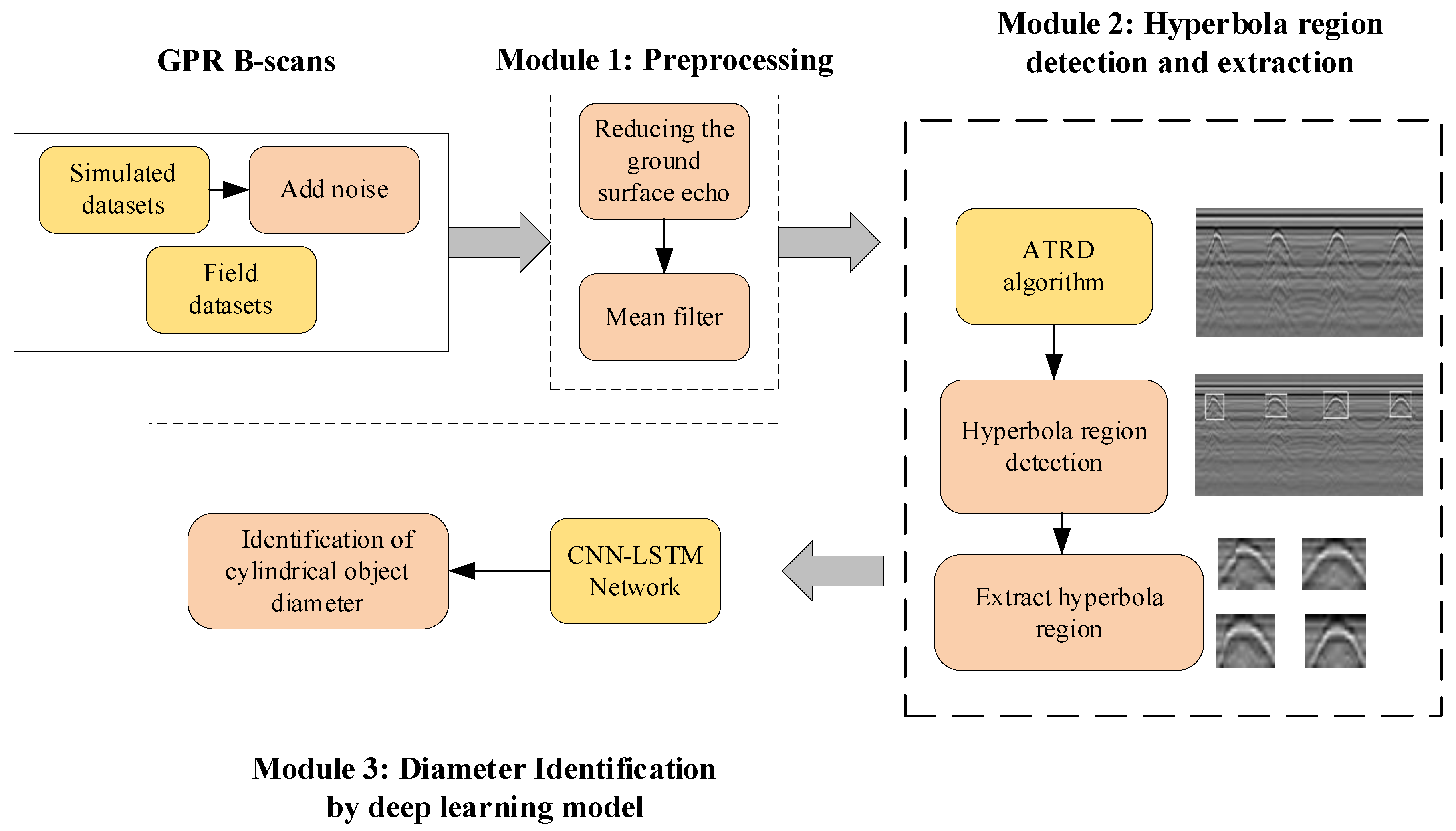
In order to solve these challenges, an automatic scheme based on the adaptive target region detection (ATRD) algorithm and Convolutional Neural Network-Long Short-Term Memory (CNN-LSTM) framework is proposed to interpret GPR data. Its flowchart is shown in Figure 1, which consists of three modules: the data preprocessing module, hyperbola region detection module, and diameter identification module. The hyperbola region in GPR B-scans can be extracted by using the ATRD algorithm, after that, the CNN-LSTM framework integrates CNN and LSTM structures to extract hyperbola region features and transfer the diameter estimation task to the hyperbola region classification task.

The contributions of this paper are summarized as follows:

(1)

The development of a scheme for diameter identification of underground cylindrical objects based on image processing and DL techniques.

(2)

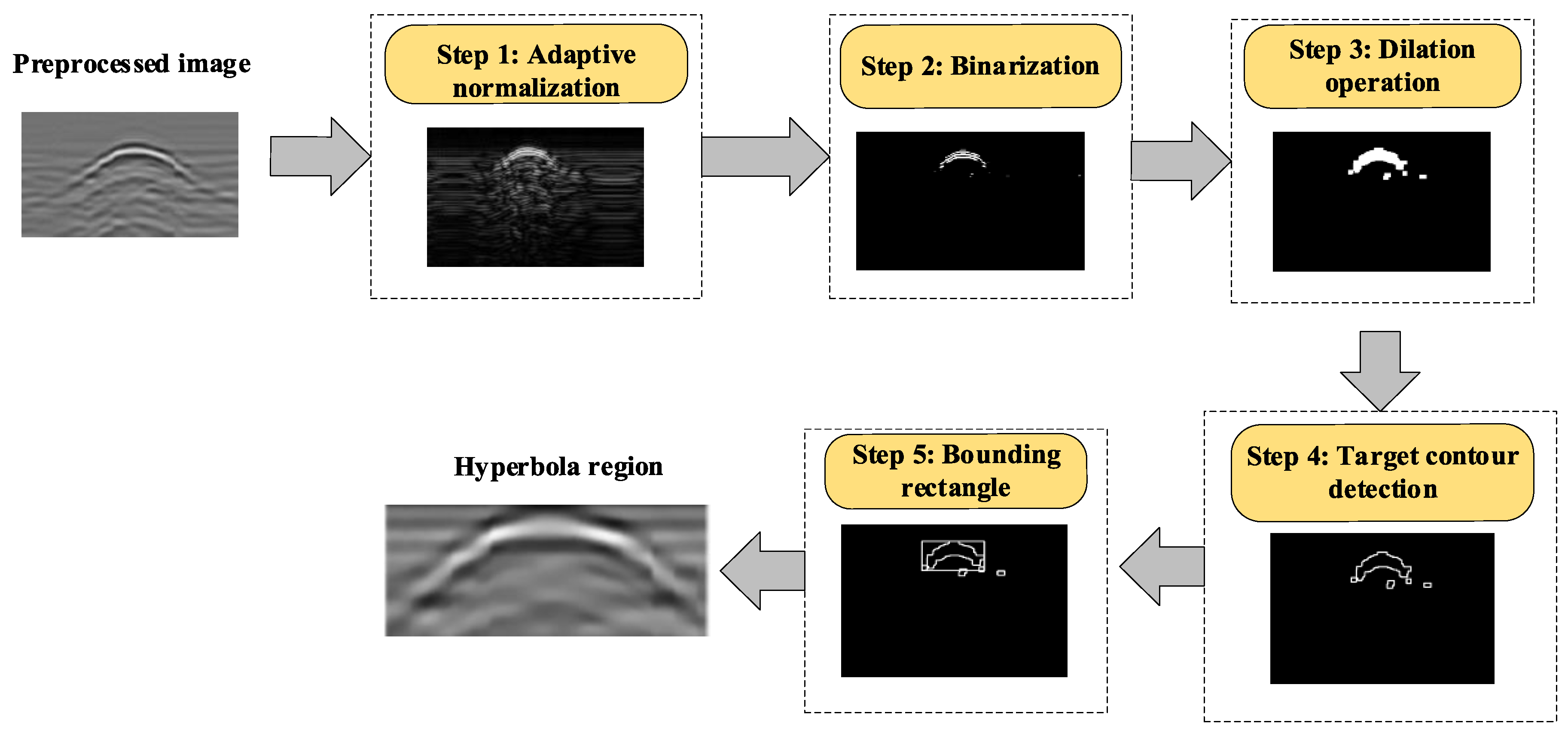
Designing an ATRD algorithm for hyperbola region detection from B-scans.

(3)

Designing a CNN-LSTM framework for diameter identification.

2. Hyperbola Region Detection via the ATRD Algorithm

In this section, the proposed ATRD algorithm is described in steps for hyperbola region detection. Before applying the proposed detection method, a series of preprocessing techniques are employed on GPR B-scans.

2.1. Preprocessing

In the preprocessing, the ensemble mean of each row is subtracted to eliminate the bright ground surface reflectance strip from a B-scan image, formulated as:

$${\widehat{S}}_{mn}=S_{mn}-\frac{1}{N}{\displaystyle {\sum }_{n=1}^N{S}_{mn},m=1,\dots ,M;n=1,\dots ,N}$$

(1)

where $S_{mn}$ represents the value of row m and column n on the original GPR B-scan. ${\widehat{S}}_{mn}$ represents the value of row m and column n on the processed GPR B-scan. Subsequently, a moving average filter processing is used to reduce the noise. An example B-scan after the preprocessing is visualized in Figure 2.

2.2. Adaptive Target Region Detection Algorithm

The proposed adaptive target region detection (ATRD) algorithm consists of five steps and its flowchart is shown in Figure 3. First, an adaptive normalization step is applied to the preprocessed B-scan and then a threshold value is selected based on the results of the experiment. Using the threshold, the normalized B-scan is converted into a binary image. Then, a dilation operation is applied to this binary image. After that, the boundary tracking method [37] is applied for contour detection of the target in the B-scan, and the bounding box of the hyperbola region is detected by the bounding rectangle method [38]. The specific steps of the ATRD algorithm are as follows.

Step 1: Adaptive normalization. An adaptive proportional coefficient is designed to normalize the preprocessed GPR B-scans. By adopting the tanh function and designing an adaptive proportional coefficient, the amplitude of background echo can be limited to near 0 and highlight underground object echo. A GPR B-scan consists of multiple A-scans. In Figure 4, a GPR A-scan is linearly transformed to [−2,2] through the adaptive proportional coefficient k, and then is non-linearly converted to [−1,1] by the tanh function. By comparing Figure 4a with Figure 4c, it can be found that the background echo is near 0, while the object echo is enhanced. The coefficient k is obtained by calculating the ratio between 2 and the peak value. However, there may be a lot of noise in the B-scan image: the peak value of the object echo may match the maximum value of the noise. In order to reduce the influence of the noise, it takes the average of top I maximum values of the object echo in B-scan. By using the absolute value function, the amplitude range of the whole echo is converted to [0,1]. A GPR B-scan matrix is expressed as A, and the adaptive normalization method is described as follows:

$$B_{mn}=\left|\frac{1-e^{-2k{A}_{mn}}}{1+e^{-2k{A}_{mn}}}\right|$$

(2)

where $k=\frac{2I}{{\displaystyle {\sum }_{i=1}^{I}A(i)}}$, $A(i)$ represents the i-th maximum value in A, I = 10, and $A_{mn}$ indicates the value of row m and column n in A.

Step 2: Binarization. The threshold selection is critical for the normalized GPR B-scans. The Intersection over Union (IoU) indicator is used to select the threshold.

IoU is the most commonly used indicator in object detection tasks. It can reflect the distance between the detection region and the real region (or ground-truth). The larger the IoU value, the closer the detection region is to the real region and the better the obtained detection effect. The definition of IoU is as follows:

$$IoU=\frac{\left|X\cap Y\right|}{\left|X\cup Y\right|}$$

(3)

Figure 5a shows the diagram of IoU calculation. Figure 5b gives the performance of hyperbola detection under different thresholds. R represents the detected region and G indicates the real region. It can obtain the largest IoU value when the threshold is 0.7, meanwhile, the detected region is closest to the real region. Figure 5c shows the IoU values under different thresholds.

Through experimental comparison, we set the threshold of 0.7 to obtain a binary image, which can be expressed by the formula:

$$C_{mn}=\{\begin{array}{l}1,B_{mn}\ge 0.7\\ 0,B_{mn}<0.7\end{array}$$

(4)

where $B_{mn}$ represents the value of row m and column n in the normalized B-scan, and $C_{mn}$ represents the value of row m and column n in the binarized B-scan.

Step 3: Dilation operation. The dilation operations are basic morphological operations in binary image. The dilation operation is used to connect regions of similar characteristics. We use structure element D to expand binary image C and shift the origin of structure element D to the (m, n) position of C. D is a 5 × 5 full 1 matrix, with the origin at the center. If the intersection between D and C at (m, n) is not empty, then the pixel value of the corresponding (m, n) position of the output image is 1, otherwise it is 0. The dilation operation is expressed as follows:

$$C\oplus D=\left\{m,n|D_{mn}\cap C\ne \varphi \right\}$$

(5)

Step 4: Target contour detection. The purpose of detecting target contour is to subsequently extract the hyperbola region where the target is located. This step should only be done after GPR scans have been binarized. A number of different methods for target contour detection exist. Here, the boundary tracking algorithm [37] was selected to detect the contour of the target. Specifically, the boundary tracking algorithm derives a set of coordinate sequences of chain codes from the boundaries between 1-pixel and 0-pixel connected components (backgrounds or holes). The information extracted is the surrounding relationship between the outer boundary and the hole boundary. The outer boundary corresponds to a 1-component and the hole boundary corresponds to a 0-component to determine the topology of a particular binary image. Based on this, we can easily extract the topological structure of the image and convert the binary image into boundary representation.

Step 5: Bounding rectangle. Through the target contour information in step 4, we calculate the positive circumscribed rectangle of the contour by the bounding rectangle algorithm [38]. The top-left coordinates, width, and height of the rectangle can be obtained through the algorithm. Therefore, we can use the information to extract the target region. (e.g., hyperbola region).

3. Diameter Identification via the CNN-LSTM Framework

3.1. Overview of CNN and LSTM

Convolutional Neural Network (CNN) is a feed-forward neural network that gains success on many computer vision problems [39]. CNN generally includes three types of layers: convolution, pooling, and fully connected layers. The convolutional layers are used to find the local relations in their input. The pooling layer gradually reduces the dimension of the input. Usually, CNN consists of a stack of many convolution and pooling layers, and then the fully connected layers are used to classify the input patterns into a limited number of classes. In addition, CNN has the characteristics of weight sharing and local connection, which is suitable for extracting related local features of an input image.

Recurrent Neural Network (RNN) is a DL model that is made up of recurrent cells. These recurrent cells allow the network to remember the previous state and are often used to detect pattern sequences on time series. Long Short-Term Memory (LSTM) networks are a kind of RNNs, which design a new structure memory unit called LSTM cell to extract the time series features of the input data [40]. LSTM overcomes the defects of gradient disappearance and gradient explosion in traditional RNN, and it has better performance for feature extraction.

The LSTM network is composed of LSTM cells. The structure of the cell includes the input gate, forget gate, and output gate, as shown in Figure 6. These three control gates enable the LSTM cell to complete the operations of reading, writing, resetting, and updating long-distance historical information. The forget gate in the structure of LSTM determines how much information in the cell state at the previous moment can be transferred to the current moment. In the input gate, the tanh function is used to generate information at the current moment, and the sigmoid function is used to control how much new information can be passed to the cell state. The output gate can get the output corresponding to the current state based on the new cell state.

The LSTM network computes the mapping between input sequence $x_t$ and output sequence $h_t$, i.e., $x_t=(x_1,x_2,\dots ,x_n)$ and $h_t=(h_1,h_2,\dots ,h_n)$. The calculation equations are given as follows:

$$\{\begin{array}{l}{i}_t=\sigma (W_{xi}{x}_t+W_{hi}{h}_{t-1}+b_i)\\ f_t=\sigma (W_{xf}{x}_t+W_{hf}{h}_{t-1}+b_f)\\ o_t=\sigma (W_{xo}{x}_t+W_{ho}{h}_{t-1}+b_o)\\ {\overline{c}}_t=\tanh (W_{xc}{x}_t+W_{hc}{h}_{t-1}+b_c)\\ c_t=f_t·c_{t-1}+i_t·{\overline{c}}_t\\ h_t=o_t·\tanh (c_t)\end{array}$$

(6)

where $c_t$ is the state information of the memory cell, ${\overline{c}}_t$ is the accumulated information at the current moment, W is the weight coefficient matrix of different gates, and b is the corresponding bias term. σ and tanh are the sigmoid activation function and the hyperbolic tangent activation function, respectively.

According to the equations, it can be inferred that the current state information, $c_t$, and the previous state information, $c_{t-1}$, have a linear relationship. When the forget gate is opened, the output of the sigmoid unit is close to 1, and the gradient will not disappear. The new state information is the weighted average between the previous state information and the accumulated information at the current moment. Therefore, without considering the sequence length, when the forget gate is open, the network can remember the past state information, that is, LSTM can extract time series features.

3.2. The CNN-LSTM Architecture

The proposed framework consists of an integration of a Long Short-Term Memory (LSTM) network and a Convolutional Neural Network (CNN). LSTM can learn the before and after dependence of sequence data by introducing memory cells and a gate mechanism, which is suitable for extracting the time series features of each column signal in the GPR B-scan. CNN captures the local correlation information in the input image through a convolution kernel, which is suitable for extracting the spatial position features of hyperbola in the GPR B-scan.

The detected hyperbola regions are used as the input of the CNN-LSTM framework. We use the CNN structure to extract the spatial position feature, $f_1$, of the hyperbola region, and the LSTM structure to extract the time series feature, $f_2$, of each column signal in the hyperbola region. After that, the two extracted features are fused to generate the fusion feature, $f_3$. The fusion feature is input to a two-layer fully connected (FC) layers to reduce the dimension of features and output a vector with size 9, which represents the diameter categories. A softmax function is employed in the final FC layer for normalizing the output vector. An overview of the proposed DL architecture is shown in Figure 7.

The proposed CNN-LSTM framework includes three parts: CNN structure, LSTM structure, and fully connected structure. The configuration of the CNN-LSTM framework is shown in

Table 1. CNN-LSTM network configuration.

CNN-LSTM Configuration
Input
CNN	(Size)/(Number)	LSTM	(Number)
Conv1	k (3 × 3)/n (4)	LSTM layer 1	n (160)
Maxpool	k (2 × 2)
Conv2	k (3 × 3)/n (4)
Maxpool	k (2 × 2)
Conv3	k (3 × 3)/n (8)
Maxpool	k (2 × 2)	LSTM layer 2	n (160)
Conv4	k (3 × 3)/n (16)
Maxpool	k (2 × 2)
Conv5	k (3 × 3)/n (32)
Maxpool	k (2 × 2)
FC-100
FC-9
SoftMax

. A block of two layers: convolution and max pooling layers, is repeated five times in the CNN structure. The size of a kernel in each convolution layer is 3 × 3 with stride 1, and the number of the kernels in each layer is 4, 4, 8, 16, and 32, respectively. The kernel size of the pooling layer is 2 × 2 with stride 2, which can reduce the dimensions of the feature map. The CNN architecture is shown in Figure 8.

The LSTM structure consists of two LSTM layers, and each layer includes 160 LSTM units. In the fully connected structure, the number of hidden layer nodes is 100, and the number of output layer nodes is the number of diameter categories. Figure 9 shows the LSTM architecture.

In the network training process, we use the cross-entropy loss function to optimize the network. In order to accelerate the training process, batch normalization [41] is utilized. In addition, the L2 regularization and restricted linear unit (ReLu) activation function are used to avoid over-fitting while training. The number of weights learnt by the whole network is 143,941 (The CNN has 6292 weights, the LSTM has 96,640, and the FC has 41,009).

4. Experiment and Analysis

This section describes the computational experiments that we performed to test the effectiveness of our proposal as well as to compare it to other different networks. We have achieved the ATRD algorithm using the OpenCV and implemented our network design using the TensorFlow framework. The training stage was performed on GPU using an Intel Core i7-9700k server clocked at 3.6 GHz with 32GB RAM and a NVIDIA GeForce RTX 2070 super GPU with 8 GB (Changsha, China). We have tested our proposal on two different datasets: simulated GPR datasets and field GPR datasets.

4.1. Datasets Collection

Simulated GPR datasets collection: we used the gprMax toolbox to generate simulated GPR B-scan datasets [42]. In the simulated experiment setup, the targets in the simulated GPR B-scans were rebars with different sizes embedded inside the concrete. The common rebar diameters in civil building engineering are 6, 8, 10, 12, 16, and 20 mm. In addition, we added the diameters 18, 22, and 24 mm in our experiment. There was a total of nine different types of diameters, expressed as D6, D8, D10, D12, D16, D18, D20, D22, and D24 (Dx represents the diameter of the rebar is x mm). The cover thickness of each rebar was designed from 30 to 130 mm and each GPR B-scan was simulated at an interval of 1 mm. Each category can generate 100 GPR B-scans. Therefore, 900 GPR B-scans can be obtained. We added two random noises to each GPR B-scan, so that a total of 1800 GPR B-scans can be generated. The datasets were divided into two parts: training set and testing set. There were 1400 GPR B-scan datasets for training and 400 GPR B-scan datasets for testing.

Field GPR datasets collection: we used GPR equipment to collect field datasets. In the field experiment setup, the buried objects in the field GPR B-scans were rebars with different sizes embedded inside the dry sand, as shown in Figure 10. Only one rebar was embedded in the dry sand in each data recording. The diameter types of rebars are the same as the simulation experiment. There was a total of nine types of diameter, expressed as D6, D8, D10, D12, D16, D18, D20, D22, and D24. The depth C of the rebar in the dry sand varied randomly from 30 to 60 mm and a GPR B-scan was recorded for each random location. Each diameter category recorded 100 GPR B-scans. We obtained 900 GPR B-scans. In addition, we used the data augmentation strategy to add two random noises to each generated B-scan, so that a total of 1800 GPR B-scans could be obtained. The datasets were divided into two parts: training set and testing set. There were 1400 GPR B-scans datasets for training and 400 GPR B-scans datasets for testing.

4.2. Experimental Result

Table 2. Confusion matrix obtained by CNN-LSTM on simulated datasets.

Diameter	D6	D8	D10	D12	D16	D18	D20	D22	D24
D6	1.00	0.00	0.00	0.00	0.00	0.00	0.00	0.00	0.00
D8	0.00	0.98	0.00	0.02	0.00	0.00	0.00	0.00	0.00
D10	0.00	0.00	1.00	0.00	0.00	0.00	0.00	0.00	0.00
D12	0.00	0.00	0.00	1.00	0.00	0.00	0.00	0.00	0.00
D16	0.00	0.00	0.00	0.00	0.98	0.00	0.00	0.02	0.00
D18	0.00	0.00	0.00	0.00	0.00	1.00	0.00	0.00	0.00
D20	0.00	0.00	0.00	0.00	0.00	0.00	1.00	0.00	0.00
D22	0.00	0.00	0.00	0.00	0.00	0.00	0.00	1.00	0.00
D24	0.00	0.00	0.00	0.00	0.00	0.00	0.00	0.00	1.00

presents the confusion matrix used to analyze the classification of 9 types of different diameters on simulated datasets. It can be seen that the proposed system is able to recognize 9 types of diameters with high accuracy, ranging from 98% to 100%. There are eight types of diameters that achieved 100% recognition accuracy, and two other diameters both achieved a recognition rate of 98%, corresponding to D8 and D16. The recognition accuracy of the overall datasets has reached 99.5%.

Table 3. Confusion matrix obtained by CNN-LSTM on field datasets.

Diameter	D6	D8	D10	D12	D16	D18	D20	D22	D24
D6	0.90	0.00	0.07	0.03	0.00	0.00	0.00	0.00	0.00
D8	0.00	1.00	0.00	0.00	0.00	0.00	0.00	0.00	0.00
D10	0.05	0.00	0.93	0.02	0.00	0.00	0.00	0.00	0.00
D12	0.07	0.00	0.00	0.79	0.00	0.09	0.00	0.05	0.00
D16	0.00	0.00	0.00	0.00	0.95	0.00	0.05	0.00	0.00
D18	0.00	0.00	0.00	0.00	0.00	0.96	0.00	0.04	0.00
D20	0.00	0.00	0.00	0.00	0.00	0.00	0.97	0.03	0.00
D22	0.00	0.00	0.00	0.00	0.00	0.00	0.04	0.94	0.02
D24	0.00	0.00	0.00	0.00	0.00	0.04	0.00	0.08	0.88

presents the confusion matrix used to analyze the classification of 9 types of different diameters on field datasets. It can be seen that the proposed system is able to recognize 9 types of diameter with high accuracy. The predicted accuracy of 7 types of diameters were more than 90%. The recognition accuracy of the overall datasets has reached 92.5%.

4.3. Performance Comparison

In this work, we integrated CNN and LSTM structures to extract the spatial position features and capture the time series features of GPR B-scans. In order to verify the validity of the combination of CNN and LSTM, we compared the accuracy of the extracting features using CNN-LSTM and extracting features using only CNN or LSTM. For fair comparison, the structure and parameters of CNN and LSTM were set to be consistent. The experiments were conducted on the same simulated datasets and filed datasets. For providing a more intuitive comparison,

Table 4. Comparison of different networks on overall accuracy and training time cost.

Methods	Simulated Datasets			Field Datasets
	Accuracy	Train Epoch	Time Cost (s)	Accuracy	Train Epoch	Time Cost (s)
LSTM only	95.5%	300	603.6	85.0%	100	304.1
CNN only	85.0%	300	60.8	90.0%	100	22.7
CNN + LSTM	99.5%	300	874.3	92.5%	100	316.8

calculated the training time cost and overall accuracy between different networks.

For the designed CNN-LSTM framework structure, Figure 11 compares different CNN networks and different LSTM networks on field datasets. The improved CNN is based on the classic Lenet-5 network. Figure 11a shows that the performance of the improved CNN is better than Lenet-5. The results in Figure 11b demonstrate that the two-layer LSTM outperforms the one-layer and three-layer LSTM on field datasets, therefore, the integration of the improved CNN and the two-layer LSTM forms a CNN-LSTM framework. The results in Figure 12 indicate that the identification accuracy of three networks all improved with the increase of epoch, and CNN-LSTM has the best accuracy performance. On simulated datasets, the final accuracy rate of the CNN-LSTM framework reaches 99.5%, followed by the LSTM (two-layer LSTM network) with an accuracy rate of 95.5%, and the CNN (improved CNN network) has the lowest accuracy rate at 85.0%. On field datasets, the final recognition accuracy of CNN-LSTM, LSTM, and CNN was 92.5%, 85.0%, and 90.0%, respectively. The confusion matrix of 9 diameters obtained by the CNN network and the LSTM network on simulated datasets are shown in

Table 5. Confusion matrix obtained by CNN network on simulated datasets.

Diameter	D6	D8	D10	D12	D16	D18	D20	D22	D24
D6	0.97	0.03	0.00	0.00	0.00	0.00	0.00	0.00	0.00
D8	0.05	0.65	0.30	0.00	0.00	0.00	0.00	0.00	0.00
D10	0.08	0.16	0.74	0.00	0.02	0.00	0.00	0.00	0.00
D12	0.00	0.00	0.00	0.94	0.06	0.00	0.00	0.00	0.00
D16	0.00	0.00	0.00	0.00	1.00	0.00	0.00	0.00	0.00
D18	0.00	0.00	0.00	0.00	0.00	0.96	0.00	0.04	0.00
D20	0.00	0.00	0.00	0.00	0.06	0.00	0.84	0.05	0.05
D22	0.00	0.00	0.00	0.00	0.00	0.00	0.14	0.86	0.00
D24	0.00	0.00	0.00	0.00	0.00	0.00	0.00	0.02	0.98

and

Table 6. Confusion matrix obtained by LSTM network on simulated datasets.

Diameter	D6	D8	D10	D12	D16	D18	D20	D22	D24
D6	1.00	0.00	0.00	0.00	0.00	0.00	0.00	0.00	0.00
D8	0.00	0.89	0.11	0.00	0.00	0.00	0.00	0.00	0.00
D10	0.02	0.18	0.80	0.00	0.00	0.00	0.00	0.00	0.00
D12	0.00	0.00	0.00	1.00	0.00	0.00	0.00	0.00	0.00
D16	0.00	0.00	0.00	0.00	1.00	0.00	0.00	0.00	0.00
D18	0.00	0.00	0.00	0.00	0.00	1.00	0.00	0.00	0.00
D20	0.00	0.00	0.00	0.00	0.00	0.00	1.00	0.00	0.00
D22	0.00	0.00	0.00	0.00	0.00	0.00	0.00	1.00	0.00
D24	0.00	0.00	0.00	0.00	0.00	0.00	0.00	0.00	1.00

.

Table 7. Confusion matrix obtained by CNN network on field datasets.

Diameter	D6	D8	D10	D12	D16	D18	D20	D22	D24
D6	0.90	0.10	0.00	0.00	0.00	0.00	0.00	0.00	0.00
D8	0.02	0.98	0.00	0.00	0.00	0.00	0.00	0.00	0.00
D10	0.02	0.00	0.98	0.00	0.00	0.00	0.00	0.00	0.00
D12	0.05	0.00	0.05	0.81	0.00	0.05	0.04	0.00	0.00
D16	0.00	0.00	0.00	0.00	0.95	0.05	0.00	0.00	0.00
D18	0.00	0.00	0.00	0.00	0.00	0.96	0.00	0.04	0.00
D20	0.00	0.00	0.00	0.00	0.00	0.00	0.95	0.05	0.00
D22	0.00	0.00	0.00	0.00	0.00	0.00	0.04	0.92	0.04
D24	0.00	0.04	0.00	0.00	0.00	0.04	0.00	0.08	0.84

and

Table 8. Confusion matrix obtained by LSTM network on field datasets.

Diameter	D6	D8	D10	D12	D16	D18	D20	D22	D24
D6	0.88	0.00	0.10	0.02	0.00	0.00	0.00	0.00	0.00
D8	0.07	0.89	0.00	0.00	0.00	0.02	0.02	0.00	0.00
D10	0.10	0.00	0.80	0.05	0.05	0.00	0.00	0.00	0.00
D12	0.00	0.05	0.05	0.81	0.00	0.07	0.00	0.00	0.02
D16	0.00	0.00	0.02	0.00	0.86	0.05	0.02	0.05	0.00
D18	0.00	0.00	0.00	0.00	0.02	0.96	0.02	0.00	0.00
D20	0.00	0.00	0.00	0.05	0.00	0.03	0.85	0.05	0.02
D22	0.00	0.00	0.00	0.00	0.00	0.04	0.06	0.85	0.05
D24	0.00	0.12	0.00	0.00	0.04	0.06	0.04	0.00	0.74

are the confusion matrix obtained by the CNN network and the LSTM network on field datasets. The performance comparison suggests that the integration of CNN and LSTM for the extraction of hyperbola features is more effective for diameter identification of underground cylindrical objects.

5. Conclusions

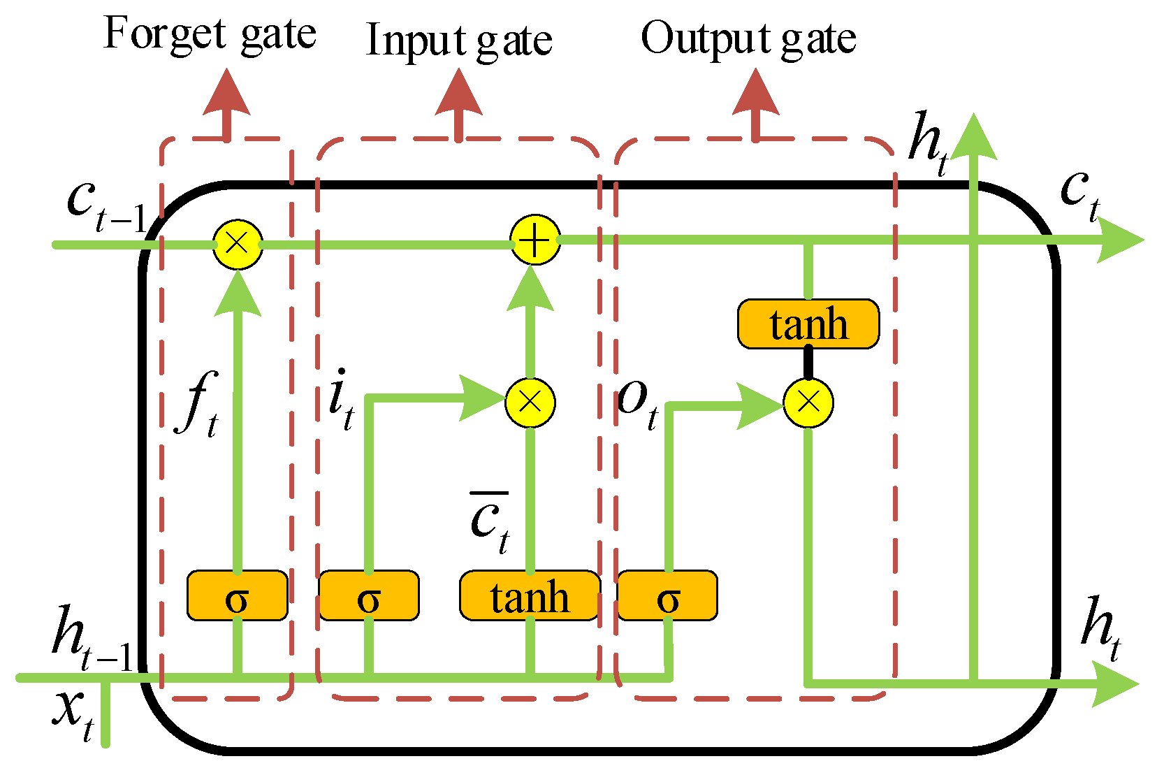
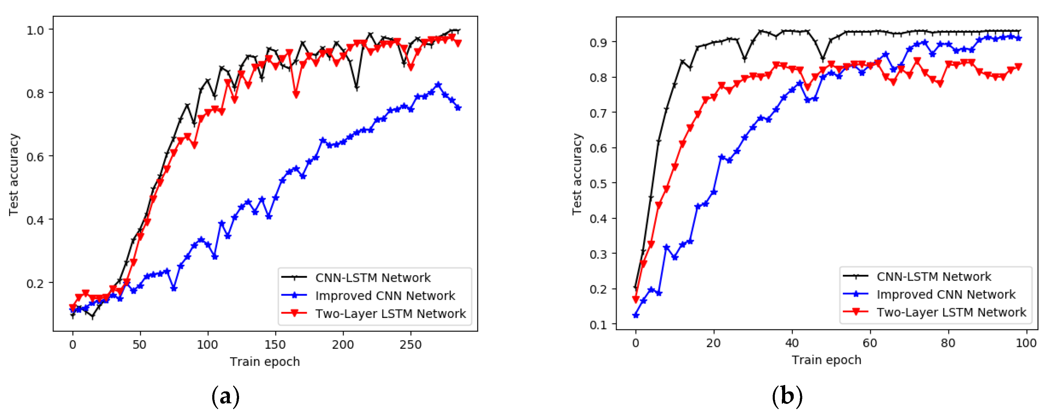
In this study, an automated scheme was proposed to identify the diameter of surface cylindrical objects in GPR B-scans. The proposed ATRD algorithm was able to extract the regions containing the expected hyperbola target from GPR B-scans. The CNN-LSTM was adopted as the main framework, which was developed to classify these regions and obtain the corresponding diameter identification results. The CNN-LSTM framework extracted both spatial position features and time series features of hyperbola regions and concatenated the two features as input of the FC layer. The comparative experiments were conducted on simulated and field datasets with nine types of diameters. The CNN-LSTM framework reached an accuracy of 99.5% on the simulated dataset and 92.5% on the field dataset, which can effectively identify different diameters of underground cylindrical objects and outperforms other DL networks. On the simulated datasets, it improved at an accuracy of 14.5% compared to the single CNN network and 4% compared to the single LSTM network. On the field datasets, it improved at an accuracy of 2.5% compared to the single CNN network and 7.5% compared to the single LSTM network.

However, the field datasets were not sufficient for the need of training the DL model. Due to the complex surface environment, it is difficult to collect and generate a large number of field data. Future work will focus on the data augmentation techniques. For example, the generative adversarial network (GAN) model could be used to generate and augment GPR datasets. In addition, the proposed scheme focuses on only the single target identification. The performance of the scheme is limited when there exists interferences or multiple targets. Future effort could be conducted to use the state-of-the-art DL network to extract the features of hyperbolic signatures with intersections with others in more complex scenarios for diameter identification.

References

1. Peters, L.; Daniels, J.; Young, J. Ground Penetrating Radar as a Subsurface Environmental Sensing Tool. Proc. IEEE 1994, 82, 1802–1822. [Google Scholar] [CrossRef] [Green Version]
2. Ostenwoldenburg, H.V.D. Applications of Ground-Penetrating Radar, Magnetic and Electrical Mapping, and Electromagnetic Induction Methods in Archaeological Investigations. In Near-Surface Geophysics; Ghose, R., Ed.; European Association of Geoscientists & Engineers: Houten, The Netherlands, 2005. [Google Scholar]
3. Wang, H.; Liu, H.; Cui, J.; Hu, X.; Sato, M. Velocity analysis of CMP gathers acquired by an array GPR system ‘Yakumo’: Results from field application to tsunami deposits. Explor. Geophys. 2018, 49, 669–674. [Google Scholar] [CrossRef]
4. Torrione, P.A.; Morton, K.D.; Sakaguchi, R.; Collins, L.M. Histograms of oriented gradients for landmine detection in ground-penetrating radar data. IEEE Trans. Geosci. Remote. Sens. 2013, 52, 1539–1550. [Google Scholar] [CrossRef]
5. Liu, H.; Sato, M. In situ measurement of pavement thickness and dielectric permittivity by GPR using an antenna array. NDT and E Int. 2014, 64, 65–71. [Google Scholar] [CrossRef]
6. Dinh, K.; Gucunski, N.; Duong, T.H. An algorithm for automatic localization and detection of rebars from GPR data of concrete bridge decks. Autom. Constr. 2018, 89, 292–298. [Google Scholar] [CrossRef]
7. Feng, Z.; Zhongchang, C.; Hai, L.; Jie, C.; Billie, S.; Guangyou, F. Simultaneous estimation of rebar diameter and cover thickness by a GPR-EMI dual sensor. Sensors 2018, 18, 2969. [Google Scholar]
8. Abouhamad, M.; Dawood, T.; Jabri, A.; Alsharqawi, M.; Zayed, T. Corrosiveness mapping of bridge decks using image-based analysis of GPR data. Autom. Constr. 2017, 80, 104–117. [Google Scholar] [CrossRef]
9. Feng, J.; Su, Y.; Ding, C.; Xing, S.; Dai, S.; Zou, Y. Dielectric properties estimation of the lunar regolith at CE-3 landing site using lunar penetrating radar data. Icarus 2017, 284, 424–430. [Google Scholar] [CrossRef]
10. Sham, J.F.C.; Lai, W.W.L. Development of a new algorithm for accurate estimation of GPR’s wave propagation velocity by common-offset survey method. NDT E Int. 2016, 83, 104–113. [Google Scholar] [CrossRef]
11. Prego, F.J.; Solla, M.; Puente, I.; Arias, P. Efficient GPR data acquisition to detect underground pipes. NDT E Int. 2017, 91, 22–31. [Google Scholar] [CrossRef]
12. Benedetto, A.; Pajewski, L. Civil Engineering Applications of Ground Penetrating Radar; Springer Nature Switzerland AG: Charm, Switzerland, 2015. [Google Scholar]
13. Shihab, S.; Al-Nuaimy, W. Radius estimation for cylindrical objects detected by ground penetrating radar. Subsurf. Sens. Technol. Appl. 2005, 6, 151–166. [Google Scholar] [CrossRef]
14. Ponti, C.; Santarsiero, M.; Schettini, G. Time-domain electromagnetic scattering by buried dielectric objects with the cylindrical-wave approach for GPR modelling. Electronics 2020, 9, 421. [Google Scholar] [CrossRef] [Green Version]
15. Ristic, A.V.; Petrovački, D.; Govedarica, M. A new method to simultaneously estimate the radius of a cylindrical object and the wave propagation velocity from GPR data. Comput. Geosci. 2009, 35, 1620–1630. [Google Scholar] [CrossRef]
16. Lester, J.; Bernold, L.E. Innovative process to characterize buried utilities using Ground Penetrating Radar. Autom. Constr. 2007, 16, 546–555. [Google Scholar] [CrossRef]
17. Capineri, L.; Grande, P.; Temple, J.A.G. Advanced image-processing technique for real-time interpretation of ground-penetrating radar images. Int. J. Imaging Syst. Technol. 1998, 9, 51–59. [Google Scholar] [CrossRef]
18. Asadi, P.; Gindy, M.; Alvarez, M.; Asadi, A. A computer vision based rebar detection chain for automatic processing of concrete bridge deck GPR data. Autom. Constr. 2020, 112, 103106. [Google Scholar] [CrossRef]
19. Illingworth, J.; Kittler, J. A survey of the Hough transform. Comput. Vis. Graph. Image Process. 1988, 44, 87–116. [Google Scholar] [CrossRef]
20. Noreen, T.; Khan, U.S. Using pattern recognition with HOG to automatically detect reflection hyperbolas in ground penetrating radar data. In Proceedings of the 2017 International Conference on Electrical and Computing Technologies and Applications (ICECTA), Ras Al Khaimah, UAE, 21–23 November 2017. [Google Scholar]
21. Bugarinović, Ž.; Pajewski, L.; Ristić, A.; Vrtunski, M.; Govedarica, M.; Borisov, M. On the introduction of canny operator in an advanced imaging algorithm for real-time detection of hyperbolas in ground-penetrating radar Data. Electronics 2020, 9, 541. [Google Scholar]
22. Bivalkar, M.; Singh, D.; Kobayashi, H. Entropy-based low-rank approximation for contrast dielectric target detection with through wall imaging system. Electronics 2019, 8, 634. [Google Scholar] [CrossRef] [Green Version]
23. Al-Nuaimy, W.; Huang, Y.; Nakhkash, M.; Fang, M.; Nguyen, V.; Eriksen, A. Automatic detection of buried utilities and solid objects with GPR using neural networks and pattern recognition. J. Appl. Geophys. 2000, 43, 157–165. [Google Scholar] [CrossRef]
24. Harkat, H.; Ruano, A.E.; Ruano, M.G.; Bennani, S.D. GPR target detection using a neural network classifier designed by a multi-objective genetic algorithm. Appl. Soft Comput. 2019, 79, 310–325. [Google Scholar] [CrossRef]
25. Lei, W.; Jiang, X.; Xu, L.; Luo, J.; Xu, M.; Hou, F. Continuous gesture recognition based on time sequence fusion using mimo radar sensor and deep learning. Electronics 2020, 9, 869. [Google Scholar] [CrossRef]
26. Yuan, D.; An, Z.; Zhao, F. Gray-statistics-based twin feature extraction for hyperbola classification in ground penetrating radar images. Procedia Comput. Sci. 2019, 147, 567–573. [Google Scholar] [CrossRef]
27. Lei, W.; Hou, F.; Xi, J.; Tan, Q.; Xu, M.; Jiang, X.; Liu, G.; Gu, Q. Automatic hyperbola detection and fitting in GPR B-scan image. Autom. Constr. 2019, 106, 102839. [Google Scholar] [CrossRef]
28. Liu, H.; Lin, C.; Cui, J.; Fan, L.; Xie, X.; Spencer, B.F., Jr. Detection and localization of rebar in concrete by deep learning using ground penetrating radar. Autom. Constr. 2020, 118, 103279. [Google Scholar] [CrossRef]
29. Jazayeri, S.; Kruse, S.; Hasan, I.; Yazdani, N. Reinforced concrete mapping using full-waveform inversion of GPR data. Constr. Build. Mater. 2019, 229, 117102. [Google Scholar] [CrossRef]
30. Jazayeri, S.; Klotzsche, A.; Kruse, S. Improving estimates of buried pipe diameter and infilling material from ground-penetrating radar profiles with full-waveform inversion. Geophysics 2018, 83, H27–H41. [Google Scholar] [CrossRef]
31. Zhang, P.; Muhammat, N. A new method on probing and interpreting underground pipeline’s diameter by GPR. In Proceedings of the Geo Shanghai 2014, Shanghai, China, 26–28 May 2014. [Google Scholar]
32. Shihab, S.; Alnuaimy, W. Hyperbola Fitter for Characterisation of Cylindrical Targets in GPR Data. In Proceedings of the 11th International Conference on Ground Penetrating Radar, Columbus, OH, USA, 19–22 June 2006. [Google Scholar]
33. Dou, Q.; Wei, L.; Magee, D.R.; Cohn, A.G. Real-time hyperbola recognition and fitting in GPR data. IEEE Trans. Geosci. Remote. Sens. 2016, 55, 51–62. [Google Scholar] [CrossRef] [Green Version]
34. Fitzgibbon, A.W.; Pilu, M.; Fisher, R.B. Direct least squares fitting of ellipses. IEEE Trans. Pattern Anal. Mach. Intell. 1999, 21, 476–480. [Google Scholar] [CrossRef] [Green Version]
35. Dolgiy, A.; Dolgiy, A.; Zolotarev, V. Optimal radius estimation for subsurface pipes detected by ground penetrating radar. In Proceedings of the 11th International Conference on Ground Penetrating Radar, Columbus, OH, USA, 19–22 June 2006. [Google Scholar]
36. Wiwatrojanagul, P.; Sahamitmongkol, R.; Tangtermsirikul, S.; Khamsemanan, N. A new method to determine locations of rebars and estimate cover thickness of RC structures using GPR data. Constr. Build. Materials 2017, 140, 257–273. [Google Scholar] [CrossRef]
37. Suzuki, S.; Be, K. Topological structural analysis of digitized binary images by border following. Comput. Vis. Graph. Image Process. 1985, 30, 32–46. [Google Scholar] [CrossRef]
38. OpenCV Reference Guide. Available online: http://docs.opencv.org (accessed on 20 May 2020).
39. Lecun, Y.; Bengio, Y.; Hinton, G. Deep learning. Nature 2015, 521, 436–444. [Google Scholar] [CrossRef] [PubMed]
40. Hochreiter, S.; Schmidhuber, J. Long short-term memory. Neural Comput. 1997, 9, 1735–1780. [Google Scholar] [CrossRef]
41. Ioffe, S.; Szegedy, C. Batch Normalization: Accelerating Deep Network Training by Reducing Internal Covariate Shift. arXiv 2015, arXiv:1502.03167. [Google Scholar]
42. Warren, C.; Giannopoulos, A.; Giannakis, I. gprMax: Open source software to simulate electromagnetic wave propagation for Ground Penetrating Radar. Comput. Phys. Commun. 2016, 209, 163–170. [Google Scholar] [CrossRef] [Green Version]
Figure 1. Illustration of GPR B-scans’ interpretation by the proposed scheme.
Electronics 09 01804 g001
Figure 2. Preprocessing results. (a) Original B-scan. (b) Preprocessed B-scan.
Electronics 09 01804 g002
Figure 3. Flowchart of ATRD algorithm for hyperbola region detection.
Electronics 09 01804 g003
Figure 4. Adaptive normalization: (a) GPR A-scan signal with noise, (b) Tanh function curve, (c) GPR A-scan signal after the adaptive normalization.
Electronics 09 01804 g004
Figure 5. Threshold selection. (a) IoU calculation, (b) hyperbola region detection results under different thresholds, (c) IoU value under different thresholds.
Electronics 09 01804 g005
Figure 6. The architecture of a Long Short-Term Memory (LSTM) cell.
Electronics 09 01804 g006
Figure 7. The architecture of the Convolutional Neural Network (CNN)-LSTM framework.
Electronics 09 01804 g007
Figure 8. The CNN architecture with the input of the hyperbola region.
Electronics 09 01804 g008
Figure 9. The LSTM architecture with the input of the hyperbola region.
Electronics 09 01804 g009
Figure 10. The setup of the field experiment.
Electronics 09 01804 g010
Figure 11. Test accuracy of different networks on field datasets: (a) Lenet-5 and improved CNN, (b) One-layer, two-layer, and three-layer LSTM network.
Electronics 09 01804 g011
Figure 12. Test accuracy of different networks on (a) simulated datasets and (b) field datasets.
Electronics 09 01804 g012