Content Estimation of Foreign Fibers in Cotton Based on Deep Learning

Abstract

Cotton foreign fibers directly affect the quality of a textile product; the less foreign fibers in raw cotton, the higher the quality grade of the textile product. Based on the foreign fiber clean machine, this paper proposed an evaluation method of foreign fiber content using deep learning. First of all, a large number of images of foreign fibers were collected from different production lines and annotated to obtain the mask image dataset of foreign fibers. Secondly, by comparing the image segmentation algorithm based on deep learning, tests showed that U-Net has a better performance on different segment metrics evaluations, and U-Net is improved to realize the real-time segmentation of foreign fiber images. The actual size of the foreign fiber could be calculated through the combination of the segment result and the mechanical parameters of the machine. Finally, the test results showed that the relative error between the estimated size and the actual size was less than 4%. After the prototype test, the algorithm was deployed on the actual production line and, by comparing the algorithm data in a random time with the actual foreign fiber statistical data, the overall error was less than 2%. The test showed that the new evaluation method can fully reflect the content of foreign fiber in raw cotton.

1. Introduction

Cotton foreign fiber (foreign fiber for short) refers to non-cotton fiber and natural cotton fiber which is mixed into raw cotton, like chemical fiber, hair, silk, hemp, plastic film, plastic rope, and dyeing thread (rope, cloth) [1]. The less foreign fiber in raw cotton, the higher the corresponding textile grade is. At present, there is no universally accepted, unified standard for the evaluation of foreign fiber content in the world. In the standard of GB1103-2012, the detection method of foreign fiber content is as follows. During processing, samples of about 2 kg are randomly selected from every 10 bales of cotton from the same pile and the same production line on the same day. All samples are combined as the batch sample of the corresponding cotton bale for the foreign fiber content inspection. This inspection method is mainly done manually. Due to the limitations of the human eye, such as inevitable eye fatigue, the small foreign fibers cannot be easily found in the cotton pile, resulting in inaccurate detection of foreign fiber content manually. Besides that, the inspection method specified in the national standard is only sampling tests, and the data is often not comprehensive enough.

With the development of the image process, a foreign fiber detection machine based on machine vision is widely used in cotton mills. This type of machine collects cotton flow images through a camera and detects targets that match the characteristics of foreign fiber, based on image processing algorithms [2]. In the process of foreign fiber detection, the count of foreign fiber can be detected, and the content of foreign fiber can be quantitatively estimated. However, this method cannot accurately reflect the true content of foreign fiber. The larger the size of the foreign fiber is, the more serious the impact on the subsequent yarn is. Therefore, to accurately evaluate the content of foreign fiber, it is necessary to make a statistical analysis of the size of foreign fiber.

If we want to estimate the size of the foreign fiber, the segmentation and morphological processing of the foreign fiber image are necessary. Then, we can calculate the actual size of each pixel, combined with the mechanical parameters of the camera, and finally get its length or area. Due to the complexity of the foreign fiber in the image, many hybrid feature representations in the target detection field have been introduced into the foreign fiber image segmentation algorithm, such as color representation, regional distribution, and morphology [3,4]. Li [5] described foreign fiber through color features, shape, and texture features, and proposed the application of a multi-class support vector machine (MSVM) in foreign fiber classification. The classification accuracy can reach 80% on the sample set. In the extraction of foreign fiber image features, Zhao [6] proposed an improved ant colony algorithm to find the global optimal features through the three basic features of color, texture, and shape. Compared with the basic ant colony algorithm, it not only reduces the number of feature sets, but also improves the classification accuracy. However, these classic image segmentation or classification algorithms rely on algorithm researchers to design feature extracting methods. If the production line changes, the image features usually need to be redesigned and re-extracted, resulting in some difficulty in the versatility of the algorithm and product promotion. At present, the image segmentation algorithm based on artificial intelligence has achieved good results in various fields. This method does not rely on artificially designed features, but effectively extracts the features of the trained target image through the most widely used deep learning technology in the current artificial intelligence algorithm [7].

Jonathan [8] used the fully convolutional network (FCN) in deep learning to train public databases, such as PASCAL VOC [9], and combined image information from shallow and fine layers to produce an accurate segmentation model. Compared with the classic segmentation model of Pascal VOC in 2012, the mean IoU (Intersection over Union) is increased by 20%. Based on the FCN, Olaf [10] proposed a U-Net (network structure similar to a U-shape) network structure, and the feature extraction part used the classic VGG (Visual Geometry Group) network [11]. However, compared with the FCN, U-Net merged feature parameters with the same number of channels, corresponding to the feature extraction part in the upsampling process, and achieves excellent results in medical image segmentation. Based on Faster RCNN (Faster Region-Convolutional Neural Network), He [12] added a branch based on a full convolution network to generate an object mask. At the same time, the pooling operation in the target area was modified to alignment operation, which was used to deal with the mismatch between the mask and the target in the original image, and the target segmentation result image was more refined. In the field of industrial detection, Rahat [13] et al. presented a new approach for automated fault detection and isolation (FDI) based on deep learning. The algorithm could diagnose multiple types of faults of automatic instrument cluster systems under real-time conditions. Dimitriou et al. [14] (in 2019) used rexpression net (R-Net), a three-dimensional (3-D) volatile neural network (3DCNN) to estimate the glue volume, instead of the traditional manual detection. The system improved PCB (Printed Circuit Board) production efficiency. Additionally, in 2020, they proposed an architecture based on a three-dimensional convolutional neural network (3DCNN) to simulate geometric changes in manufacturing parameters and predict impending events related to suboptimal performance [15]. It can be effectively used for defect prediction on the PCB dataset they have published. Based on the domain fluctuation adaptive deep ensemble learning method, a distributed difference recognizer based on data set distribution and data feature estimation was proposed by Liu et al. [16]. This method has good adaptability and robustness in industrial flow data scenarios. Regarding the foreign fiber-related image processing algorithm based on deep learning, Wei [17] implemented a real-time intelligent classifier for foreign fiber images. On a dataset of 20,000 foreign fiber images, the accuracy rate reached 95% on classification, and it was also widely used in the industrial field. Compared with classic algorithms, image processing technology based on deep learning has obvious advantages.

Based on the classifier of the sorting machine which was designed by [18], the foreign fiber image segmentation algorithm based on deep learning is added. For the mainstream segmentation networks, such as FCN, U-Net, and SegNet, various comparisons are made on the foreign fiber image dataset. Finally, the classic U-Net structure is improved by combining the characteristics of the industrial field and the image characteristics of the foreign fiber. Through a single network structure to achieve classification and segmentation at the same time, a real-time foreign fiber size estimation method is proposed to evaluate the foreign fiber content of raw cotton more comprehensively.

2. Methods

At present, FCN, U-Net, SegNet [19], Mask R-CNN, and DeepLab [20] are mainly used for image segmentation technology architecture, based on deep learning. The basic idea is to classify each pixel in the image, determine the category of each point, and then divide the area [21]. These image segmentation technologies currently have been widely used in scenarios such as autonomous driving [22,23], unmanned aerial vehicles [24], and medical diagnosis and treatment [25]. However, Mask R-CNN and DeepLab have a large number of calculations. Among them, Mask R-CNN contains Faster R-CNN detection [26], which will not be used in foreign fiber segmentation. Besides that, DeepLab uses new convolution calculators such as dilated convolution, which is difficult to implement on many general embedded hardware platforms. Considering the actual working scenario, in the following discussion, Mask R-CNN and DeepLab-related architectures are no longer introduced, and only the three networks of FCN, U-Net, and SegNet are further discussed.

The general image segmentation architecture can be considered as an encoder–decoder network, and the encoder is usually a convolutional neural network structure for feature extraction. The commonly used classic feature extraction networks [27] mainly include VGG and Res-Net [28], among others, which have obtained impressive results in various large-scale dataset classification competitions. Corresponding to the encoder is the reverse decoder network, which mainly needs to retrieve the discriminable features learned by the encoder from the image semantics to the pixel space to obtain the classification result of each pixel. For FCN, U-Net, SegNet, and other structures, the main difference is the feature integration methods of the decoder.

The classic convolution neural network (CNN) uses a fully connected layer to map the feature map, generated by the convolution layer into a feature vector of a given length, and the vector is used to obtain the classification or regression results at the image level through classic classifiers such as Softmax. For example, AlexNet [29] outputs a 1000-dimension vector, which represents the probability that the input image belongs to each of the 1000 categories of the classification target. FCN modifies the full connection layer into the convolution layer and uses deconvolution to upsample the features of the last layer in the classification network to recover the dimension as the original image. Finally, the classification prediction is processed, and the relative spatial information in the original image is retained as the segmentation result.

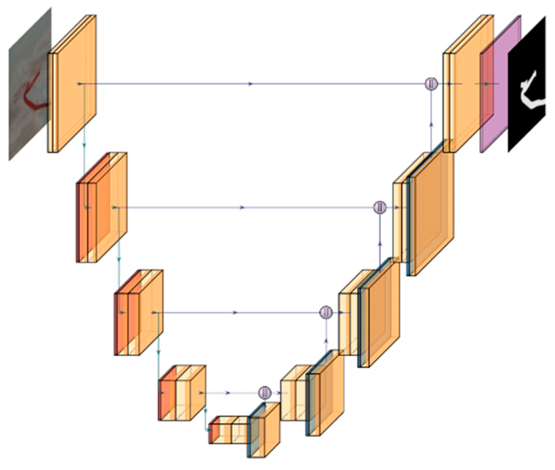
Many segmentation networks are based on the improvement of FCNs. The feature extraction part of the U-Net is the same as an FCN. In the decoder part, U-Net has made some changes. Since the overall structure is like an asymmetrical U-shape, it is called the U-Net network. The network structure is shown in Figure 1.

U-Net is mainly used for medical image segmentation, which can achieve good results on small datasets. Unlike an FCN, U-Net introduces skip connections between the encoder and the decoder, which enables the encoder and the decoder to share information. The difference between SegNet and other networks is that the pooled output values are recorded during the downsampling pooling process, and are restored during the up-pooling stage, which can improve segmentation accuracy.

In the application of cotton foreign fiber segmentation described in this paper, cotton is taken as the background, and foreign fiber is the target to be segmented. The convolution layer in the CNN has a small receptive field and extracts local features, such as the edge information of a foreign fiber image, while the deeper layer has a larger receptive field and learns the overall features, such as foreign fiber morphology, color, and texture. After being processed by the convolution layer, the encoder outputs a multichannel feature image with a very small resolution. The featured image is then sampled on the decoder and restored to the original input image resolution. Finally, the classifier is used to classify each pixel of the feature image.

3. Hardware and System

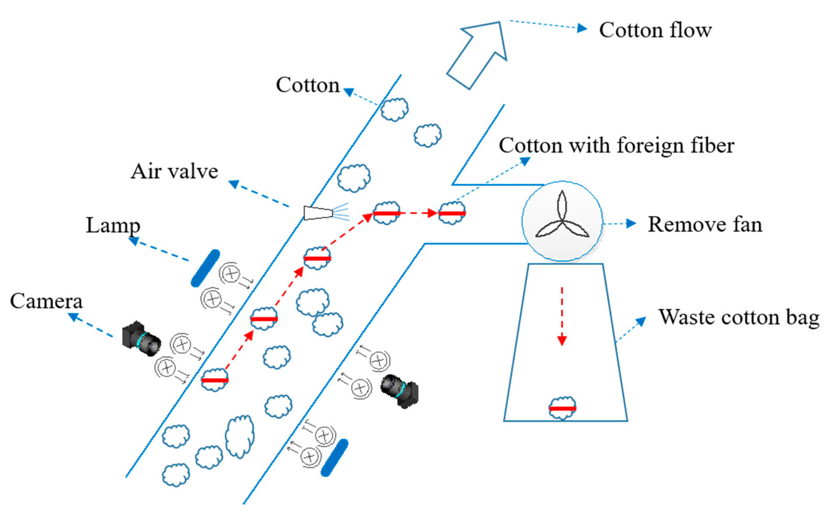
In this paper, the experimental machine is a kind of foreign fiber cleaning equipment based on machine vision [17]. In the cotton spinning production line, through the cotton flow after the opener, there is a great deal of foreign fiber attached to the surface of the cotton flow. When the cotton containing foreign fiber passes through the machine channel, the high-speed cameras transmit the collected images to the processing subsystem. After the target foreign fiber is confirmed, the high-speed air valve is used to separate the target from the cotton into the impurity removal subsystem. In the system, the airflow direction is changed by the removal fan, and the target is collected into the waste cotton bag. The system structure is shown in Figure 2. The red mark represents cotton with foreign fiber. When the image processing subsystem detects the target through the camera, the algorithm generates the corresponding removal information. The air valve subsystem uses high-pressure air and the removal fan to change the direction of the target’s movement to the waste cotton bag.

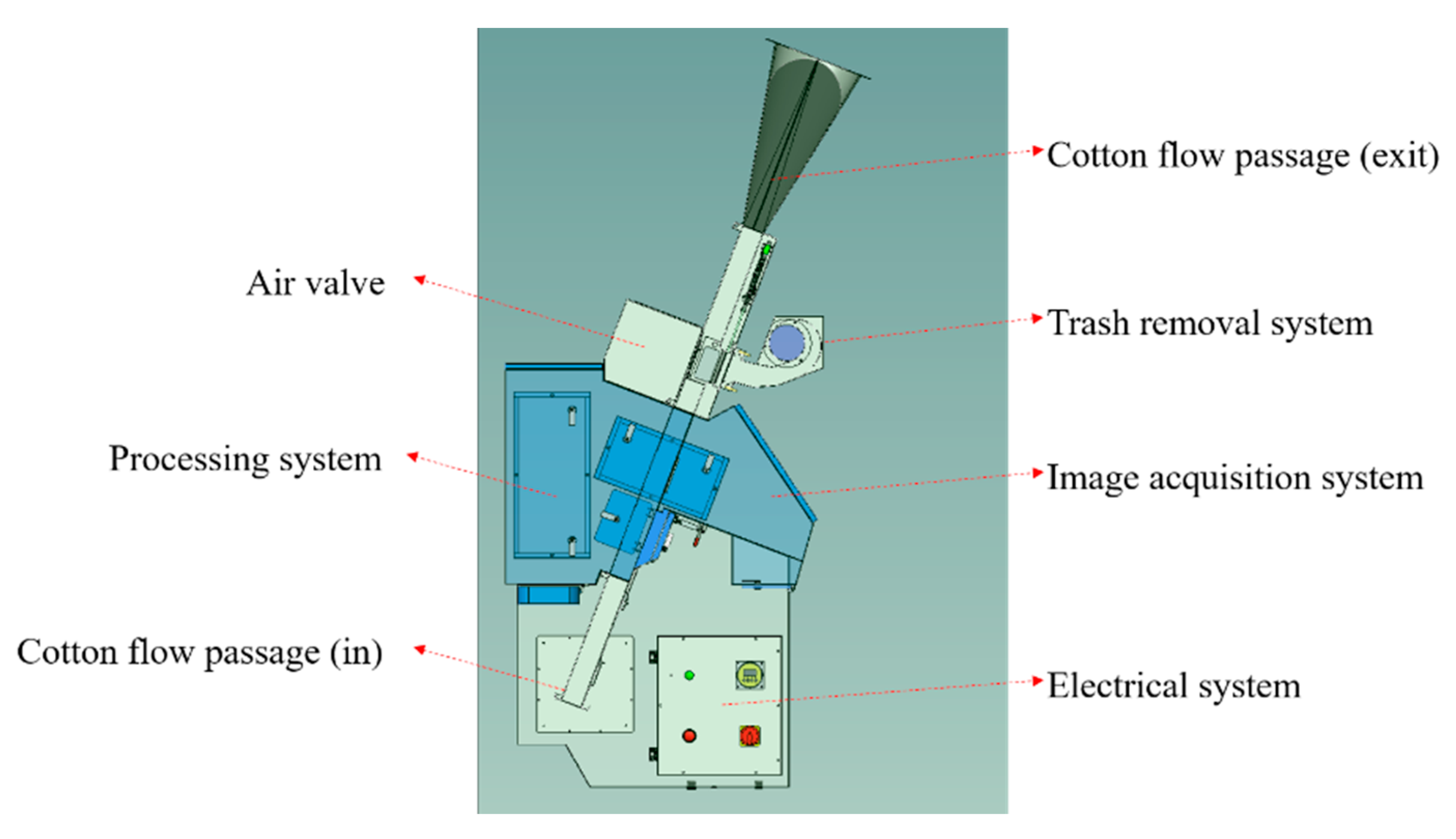
Figure 3 is the brief structure design of the foreign fiber machine. The air valve module, trash removal system, image acquisition system, image processing system, and electrical system are distributed on both sides of the cotton flow passage. The lower part of the cotton flow passage is the inlet, which is generally connected to the opener of the cotton spinning production line, and the upper part is the outlet, which is connected with the main cotton flow channel on the production line. 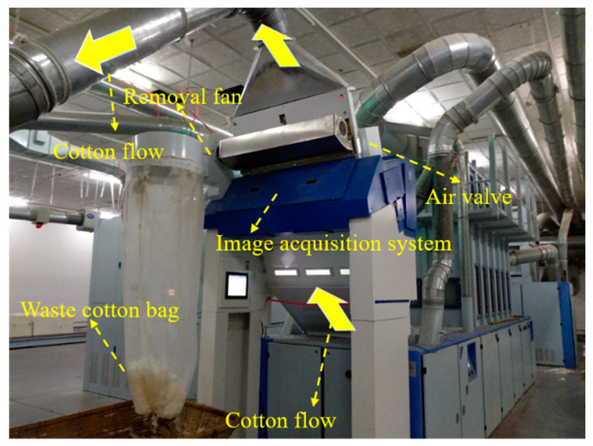Figure 4 shows the machine that is installed on the production line. The foreign fiber cleaning machine is only a part of the main cotton flow channel on the production line, and it will not contact cotton directly for processing. It only uses machine vision and relevant mechanical methods to remove the foreign fiber exposed on the surface of the cotton flow.

Considering the industrial situation, a segmentation algorithm is added to the original image classification subsystem. More computation is needed, so the classification subsystem is updated from the multicore DSP platform used in [17] to NVIDIA’s Jetson TX2 embedded platform. Jetson TX2 uses Nvidia Pascal GPU architecture, has 256 computing unified device architecture (CUDA) cores, 1.5 trillion tera floating-point operations per second (TFLOPS), and 8 GB of memory. It is currently widely used in industrial scenarios. On the hardware platform, the calculation process can also be accelerated by TensorRT.

Accurate segmentation of the images is a necessary condition for foreign fiber content evaluation. The optical part of the foreign fiber cleaning machine is relatively fixed, and the corresponding relationship between the image and the actual size can be established. The parameters of the line scan camera used in this article are described in [18]. Assuming the number of scanning lines per second for the camera is $S$, the corresponding target foreign fiber speed is $V_0$ (meters per second, or m/s), each row of pixels corresponds to a length of $V_0/S$, the shooting range of the camera in the horizontal direction is assumed to be P mm, the horizontal resolution of the camera is D, and the corresponding length of each pixel in the horizontal direction is D/P mm. The camera used in this article had 9125 sampling lines per second in the vertical direction. If the foreign fiber speed is 10 m/s, the corresponding vertical pixel length is 1.08 mm. The shooting range is usually 621 mm, which corresponds to a length of 0.296 mm per pixel in the horizontal direction when the horizontal resolution is 2096. The size of the area can be multiplied by the number of pixels and by the area of a single pixel, and the length of the linear foreign fiber is estimated according to the actual size of the pixel unit.

4. Experiment

4.1. Dataset

In this paper, the image acquisition system was based on a KL2313 CCD linear array camera [30]. The pixel frequency of each channel of the camera was 20 MHz, and after customized modification, the line frequency of the camera remained the highest at 9.2 KHz under the three-line space correction mode. A linear array camera was chosen because it had a higher resolution at the same cost when photographing moving foreign fiber in the cotton flow. The specific performance parameters of the camera are shown as follows:

• The horizontal resolution was 2096 pixels, and the maximum number of vertical sampling lines was 9195.
• The aperture of the optical system was 50 mm.
• The signal output used the Cameralink base. The maximum transmission frequency was 60 MHz.
• The dynamic range of the camera was 65 dB, which ensured the stability of the camera in an extremely harsh environment.

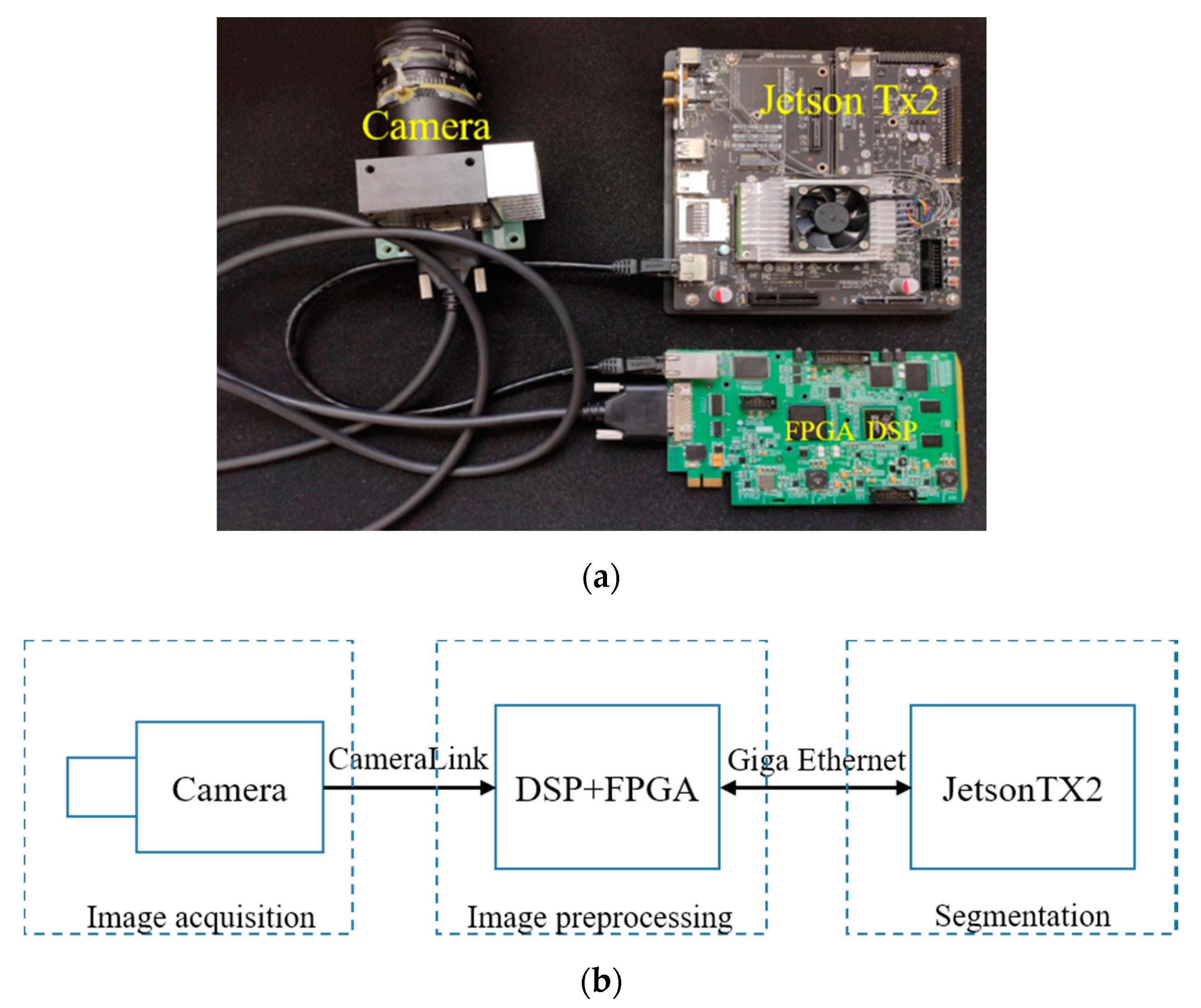
The image acquisition system used a linear array camera based on the KL2313, the preprocessing subsystem used FPGA (Field Programmable Gate Array) and DSP (Digital Signal Processor) architecture, and the Jetson TX2 was used as an AI algorithm accelerator, including CNN algorithms such as segmentation and classification based on deep learning. The preprocessing subsystem connected the camera through CameraLink. The FPGA module in the subsystem converted the original image data of the camera into a standard interface and transmitted it to the DSP. The DSP performed simple preprocessing, filtered most irrelevant images, detected targets that may have foreign fibers, and sent the images to the AI subsystem for classification or other algorithm processing based on deep learning. The hardware diagram and principle block diagram are shown in Figure 5.

The example image collected by the foreign fiber machine is shown in Figure 6. The resolution in the horizontal direction was 2096 and that in the vertical direction was 128, which is suitable for DSP memory alignment, thus accelerating the algorithm operation. We could not use the whole image as the training sample of a deep learning segmentation network. In this paper, we used slice processing to divide 2096 pixels in the horizontal direction into 18 slices of 128 pixels each, and 8–16 pixels were allowed to overlap between slices. In this way, the experimental dataset used various foreign fiber images collected during the actual commercial use of the foreign fiber cleaning machine. The main foreign fibers were colored cloth, waste paper, plastic, feathers, hair, polypropylene, and mulch film. Typically annotation samples are shown in Figure 7.

The dataset consisted of the original image and the corresponding mask image. Among the dataset, the original images were from the classified image dataset collected in [17]. The combination of semi-manual annotation and full manual annotation was used to make corresponding mask images. The mask images in Figure 7 have different gray values, which are mainly used to distinguish their categories. In the category of foreign fiber, the image features of polypropylene, animal hair, cloth, and waste paper are quite different from those of cotton. These samples with obvious features could be segmented by using a classical image algorithm, such as canny and OTSU (Maximum Between-Class Variance Method Designed by Nobuyuki Otsu). After obtaining the segmented coordinates, they could be corrected manually. The mulch film in Figure 7 was closer to cotton or the background in color space, and they needed manual annotations.

Table 1. Descriptions of the database images.

Index	Class Name	Image Count	8~12 m/s	5~8 m/s
0	Feather	6421	46%	54%
1	Cloth	5790	51%	49%
2	Waste Paper	6065	45%	55%
3	Polypropylene	5416	57%	43%
4	Mulch Film	8844	55%	45%

shows the images of foreign fiber included in the dataset used in this article.

This dataset covered the main production line speed of most cotton mills, and the amount of mulch film was more than other types, since the mulch film was hard to segment. In the deep learning training process, 80% (26,028) of each category was selected as the training set, 10% (3255) was the validation set, and 10% (3253) was the test set. The validation set was used to evaluate the segmentation effect of the three discussed algorithms, and the test dataset was used to test the generalization ability of the final algorithm.

4.2. Training and Evaluation

FCN, U-Net, and SegNet use the classification network in [17] as the encoder. This network structure has been successfully applied to commercial products, taking into account performance and computing power. Based on this structure, the encoder and decoder were designed as shown in

Table 2. Structure of the network in this paper.

Function	Filter Count	Size/Stride/Pad	Input (H/W/C)	Output (H/W/C)
Convolution	16	3/1/1	128/128/3	128/128/16
Max Pool	-	2/2/0	128/128/16	64/64/16
Convolution	32	3/1/1	64/64/16	64/64/32
Max Pool	-	2/2/0	64/64/32	32/32/32
Convolution	64	3/1/1	32/32/32	32/32/64
Max Pool	-	2/2/0	32/32/64	16/16/64
Convolution	128	3/1/1	16/16/64	16/16/128
Max Pool	-	2/2/0	16/16/128	8/8/128
Convolution	256	3/1/1	8/8/128	8/8/256
Max Pool	-	2/2/0	8/8/256	4/4/256
Convolution	512	3/1/1	4/4/256	4/4/512
Upsample	256	3/2/1	4/4/512	8/8/256
Upsample	128	3/2/1	8/8/256	16/16/128
Upsample	64	3/2/1	16/16/128	32/32/64
Upsample	32	3/2/1	32/32/64	64/64/32
Upsample	16	3/2/1	64/64/32	128/128/16
Convolution	1	1/1/0	128/128/16	128/128/1

, and the hyperparameters and training platform used in the experiment are listed in

Table 3. Hyperparameters and training platform.

Hyperparameters and Platform	Value or Name
Algorithm Optimizer	Adam
Training Epochs	200
Start Learning Rate	0.001
Momentum	0.9
Batch Size	64
CPU	Intel Xeon CPU E5-2620 v4 @ 2.10 GHz
GPU	Nvidia 1080 Ti
Memory	32 GB
Program Language	Python/C/C++

. In this paper, we used the PyTorch library as the training framework. PyTorch is an open-source machine learning framework that accelerates the path from research prototyping to production deployment. On the embedded platform, we used C/C++ mixed programming. Firstly, the PyTorch trained model was transformed into the ONNX model, which is recognized by TensorRT, and then the inference was realized on a JetsonTX2 by calling TensorRT the standard API.

While in the process of upsampling, U-Net concatenated the corresponding layer features trained in the encoder. SegNet used the max-pooling index table in the encoder to perform an upsampling recovery operation. The algorithm training optimizer used Adam optimization [31]. It was an extended version of stochastic gradient descent (SGD), and based on SGD, the concept of adaptive momentum was added in Adam for a more stable convergence training process. Adam can calculate the adaptive learning rate of each parameter through the adaptive momentum estimation method. In practical application, compared with other adaptive learning rate algorithms, the convergence speed of Adam is faster, and it avoids the problem of a local minimum. Adam can also correct the common problems existing in other optimization techniques, such as a learning rate approaching 0, gradients disappearing, the influence of different hyperparameters, and so on. It was assumed that the average gradient of the current gradient was $m_t$. The variance was ${\widehat{v}}_t$. Then, the gradient average value and variance at the next moment were calculated as in Equations (1) and (2):

$${\widehat{m}}_t= \frac{m_t}{1- {\beta }_1^{t }}$$

(1)

$${\widehat{v}}_t= \frac{v_t}{1- {\beta }_2^t}$$

(2)

where ${\beta }_1$ is 0.9 and ${\beta }_2$ is 0.9999, which are input parameters. The updated parameter is shown in Equation (3):

$${\theta }_{t+1}= {\theta }_t- \frac{\eta }{\sqrt{{\widehat{v}}_t}+ ϵ}{\widehat{m}}_t$$

(3)

where ${\theta }_t$ is the parameter at the current training time, ${\theta }_{t+1}$ is the training parameter at the next moment, and η is the learning rate. It was dynamically adjusted from large to small, according to the number of training rounds. ϵ was generally set as 0.00000001 to avoid the protection value with a denominator of 0, which had little influence in the training process. In general, the default value could be used directly for the super parameters. In the training process, the change of these parameters had a limited impact on the overall results. Moreover, because the encoder part of this paper used the same network structure as the classifier in [17], the encoder parameters could use the classifier parameters as the pre-trained weight to speed up the training process. The training curves of the three networks when the loss function was cross-entropy are shown in Figure 8. It can be seen from Figure 8 that U-Net had the fastest convergence and the lowest cross-entropy loss.

4.3. Discussion

The evaluation of the segmentation network needed to estimate the possible situation of the actual prediction results. As shown in Figure 9, the green part T₁ identifies the ground truth, T₀ is the cotton flow and blank background area under artificial annotation, the red P₁ section is the predicted foreign fiber area of the mulch film, and P₀ is the predicted cotton flow and blank background area. These four parts can be combined in four ways, and are defined as follows:

• True positive (TP) samples, which are considered to be positive samples. They are the intersection of the red parts and the green parts.
• True negative (TN) samples, which are considered as negative samples. They are also negative samples. The outside of the red and green parts is their area.
• False negatives (FNs), which are judged as negative samples, but are in fact positive samples. They are the area in the green parts, except for the red parts.
• False positives (FPs), which are judged as negative samples, but they are actually negative samples; that is, they are the area in the red parts other than the green parts.

According to the above definition, pixel accuracy (PA), recall, and the mean intersection over union (MIoU) are the most common evaluation metrics for segmented networks. Their calculation formulas are shown in Equations (4)–(6):

$$\mathrm{PA}= \frac{TP+TN}{TP+FP+TN+FN}$$

(4)

$$\mathrm{Recall}= \frac{TP}{TP+FN}$$

(5)

$$\mathrm{MIoU}= \frac{TP}{TP+FP+FN}$$

(6)

TP represents the intersection of the predicted foreign fiber and the ground truth. TN represents the intersection of the predicted cotton part. PA represents the proportion of all predicted correct pixels to the total pixels. Recall represents the proportion of correct pixels in the correct prediction results.

In some cases—for example, when the overlapping area between the prediction results and ground truth is large—PA, recall, and MIoU cannot distinguish between two objects overlapping in different ways. Referring to the field of medical segmentation, many other measurement methods could be used to evaluate the performance of the segmentation network. In the field of foreign fiber segmentation, it is impossible to use one measurement method to evaluate the segmentation performance. In order to evaluate the segmentation network completely, in addition to the above three common evaluation metrics, this paper also introduced segmentation network evaluation metrics from the medical field: Dice, Jaccard, false negative rate (FNR), and false positive rate (FPR) [32,33]. Through the above standards, the performance of the three kinds of segmentation networks was comprehensively evaluated to compare their advantages and disadvantages. Their formulas are shown in Equation (7):

$$\begin{array}{c}\mathrm{Dice}= \frac{2\left(T1 {{\displaystyle \cap }}^{ }P1\right)}{T1+P1}\\ \mathrm{RVD}= \frac{T1-P1}{T1}\\ \mathrm{FNR}= \frac{FN}{T1{{\displaystyle \cup }}^{ }P1 }, \mathrm{FPR}= \frac{FP}{T1{{\displaystyle \cup }}^{ }P1 }\end{array}$$

(7)

The Dice coefficient is a similarity measure function, which is usually used to calculate the similarity of two samples. The relative volume difference (RVD) represents the difference in volume between the predicted results and the ground truth. The FNR is the ratio of missing pixels that are segmented in the ground truth. The FPR represents the ratio of pixels to be segmented outside the ground truth.

In this paper, we selected a typical foreign fiber image and evaluated it with different network structures under the same training times, as shown in Figure 10.

Table 4. Training outputs during different epochs.

Network	FCN	U-Net	SegNet
Iteration 10
Iteration 50
Iteration 100
Iteration 200

lists the outputs of three networks for the dataset, which is shown in Figure 7, under different training epochs.

It can be seen from Table 4 that, with the increase of iterations, all networks could decode segmentation images that matched the training data. However, from the initial iterations, SegNet used the maximum pooling index to directly perform upsampling restoration work, which presented a grid effect in the output. Through the backpropagation optimization of the encoder, these grids could also be eliminated in the subsequent training to match the original segmented image. U-Net could better restore the segmented image in the decoder by concatenating the features of the encoder stage.

Table 5. Results of different evaluation metrics under different networks.

Method	MIoU	PA	Recall	Dice	RVD	FNR	FPR
FCN	85.7	93.6	88.5	80.4	10.2	6.8	9.8
U-Net	89.3	96.1	86.7	84.3	5.1	6.9	8.8
SegNet	86.4	95.1	89.5	79.8	9.5	8.2	11.9

shows the evaluation results of the three networks on the validation dataset during different metrics. It can be seen from the table that U-Net outperformed the other two networks in terms of key evaluation metrics. Due to the real-time requirements of the industrial application, in addition to satisfying the functions, it was also necessary to evaluate the time-consuming nature of the segmentation network under a given computing platform.

According to the camera parameters described in [18], the line-scan camera sampled 9195 lines per second. Assuming that 128 sampling lines were selected as one frame of data processing, the data sampling time of each frame was 13.92 milliseconds (128/9195 ms). According to the discussion in [17,18], the maximum processing time was about 5.7 milliseconds. It was assumed that the line speed of the cotton spinning was ${\upsilon }_0$ (meters per second, or m/s), and the distance between the removal valve of the foreign fiber cleaning machine and the camera shooting position was about L mm. Besides that, the valve also needed a mechanical start-up time of about $c_0$ milliseconds. The remaining processing time $T_0$ of the classification and segmentation subsystem refers to Equation (8):

$$T_0= \frac{L}{{\upsilon }_0}-c_0-13.92-5.7$$

(8)

At present, the interval distance $L$ of foreign fiber clean machine is 500 mm, the cotton spinning production line is generally about 12 m/s, and the mechanical start-up time of the valve is 16 ms. Finally, according to Equation (8), the maximum processing time of the classification and segmentation subsystem is 5.63 ms, considering some speed errors and data transmission time, the maximum processing time is set to 4 ms.

The upsampling operation of SegNet does not belong to the standard operation layer of TensorRT, and cannot be accelerated. All operations of FCN and U-Net can be accelerated by TensorRT. The inference time of the three networks and the final comparison of the same training times are shown in

Table 6. Inference time of different segment networks on JetsonTX2.

Network	Inference Time (ms)
FCN	2.94
U-Net	3.2
SegNet	5.1

.

It can be seen from Table 6 that, although the inference time of U-Net was longer than that of FCN, the mean IoU of U-Net was higher than that of FCN. SegNet cannot fully use TensorRT for acceleration, and it takes more time than the other two networks. Based on the above results, this article chose U-Net as the basic segmentation network.

4.4. Improvement

Generally, real foreign fiber needs to be segmented. The feature extraction part used by the image classification system is the same as the segmentation network encoder. Therefore, the classification and segmentation networks can be combined, the classification branch is added in the last layer of the encoder, and backpropagation is added for training. The classification and segmentation processing can be performed at the same time, which saves the calculation time of the classifier. The final U-Net segmentation network improved in this article is shown in Figure 11. The classification convolutional layer and average pooling were added to the last layer of the encoder and, finally, output the classification results by the Softmax layer. The improved U-Net can train the segmentation and classification networks at the same time, and they share the feature parameters in the encoder part. The classifier outputs the target categories to the segmented network as prior knowledge. The categories are real foreign fiber and pseudo foreign fiber. The segmented network combines the classification results in the final output results to optimize the codec parameters and speed up parameter optimization in the backpropagation. As shown in Figure 12, the experimental results show that, under the same training environment, the convergence time of the improved U-Net was less than the original U-Net. It began to decline in stability when the training epoch was 100, and the Softmax loss result was far less than 0.1, which could be used for deployment.

5. Deployment and Application

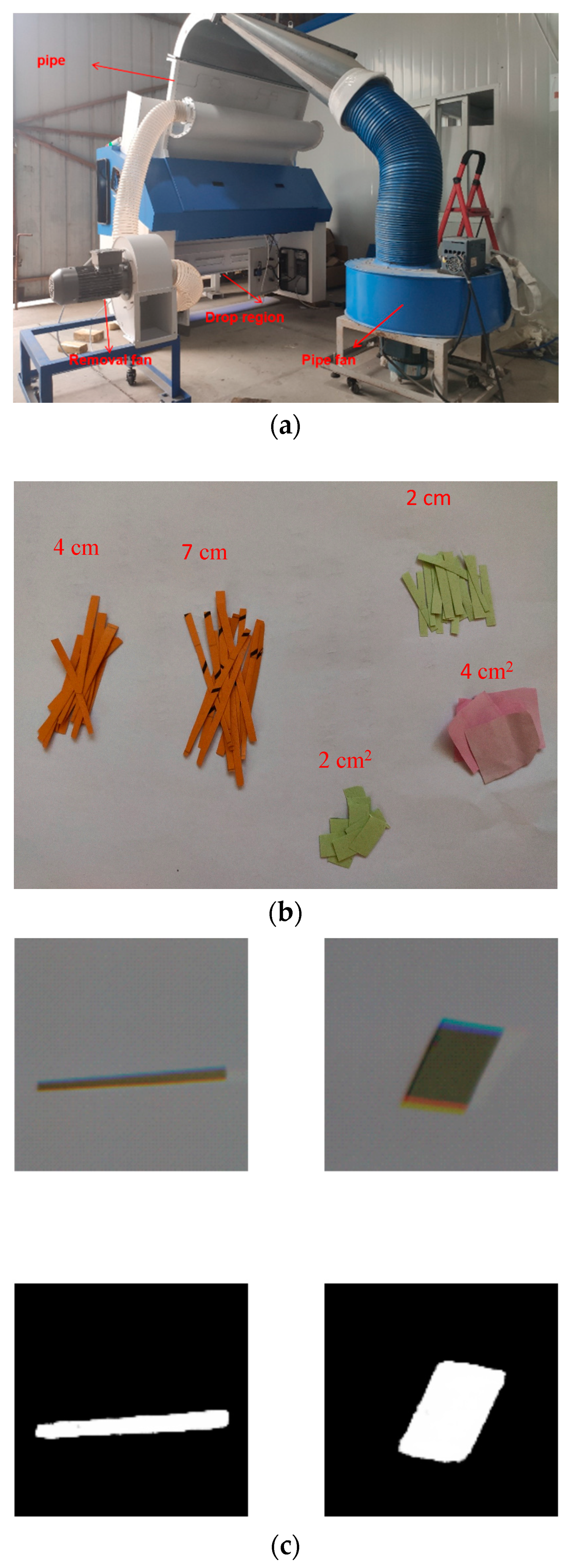
Before the algorithm is deployed to the production line, the accuracy of the algorithm needs to be tested on an experimental prototype. The experimental prototype used in this paper is shown in Figure 13a. The test samples were thrown into the pipe from the drop region. The test samples are shown in Figure 13b. Ten samples of 2 cm, 4 cm, and 7 cm, and 10 samples of 2 cm² and 4 cm² were chosen for the test. The corresponding pictures and the segmentation results are shown in Figure 13c.

The test results are shown in

Table 7. The statistics estimation of standard size samples.

Index	1	2	3	4	5	6	7	8	9	10	RMSE
2 cm	1.94	2.01	1.97	2.1	1.77	2.1	1.94	2.0	1.88	1.97	0.098 (4.9%)
4 cm	4.0	3.72	3.75	4.01	4.03	3.75	3.82	3.93	4.06	4.12	0.161 (4%)
7 cm	6.94	6.98	7.46	6.6	7.25	7.39	7.47	6.7	7.27	7.09	0.313 (4.4%)
2 cm2	2	1.85	2	1.91	1.88	1.93	1.91	2.09	2.06	1.94	0.083 (4.1%)
4 cm2	3.82	3.85	3.9	3.96	4.01	3.83	3.94	4.1	4.04	3.85	0.114 (2.85%)

. In this paper, the root mean square error (RMSE) was used to evaluate the measurement results of the algorithm. It can be seen from the table that the RMSE of five groups of tests was 4%, relative to the calibration size. Considering the correlation of image segmentation error and camera sampling characteristics, the algorithm met the actual fiber size estimation requirements.

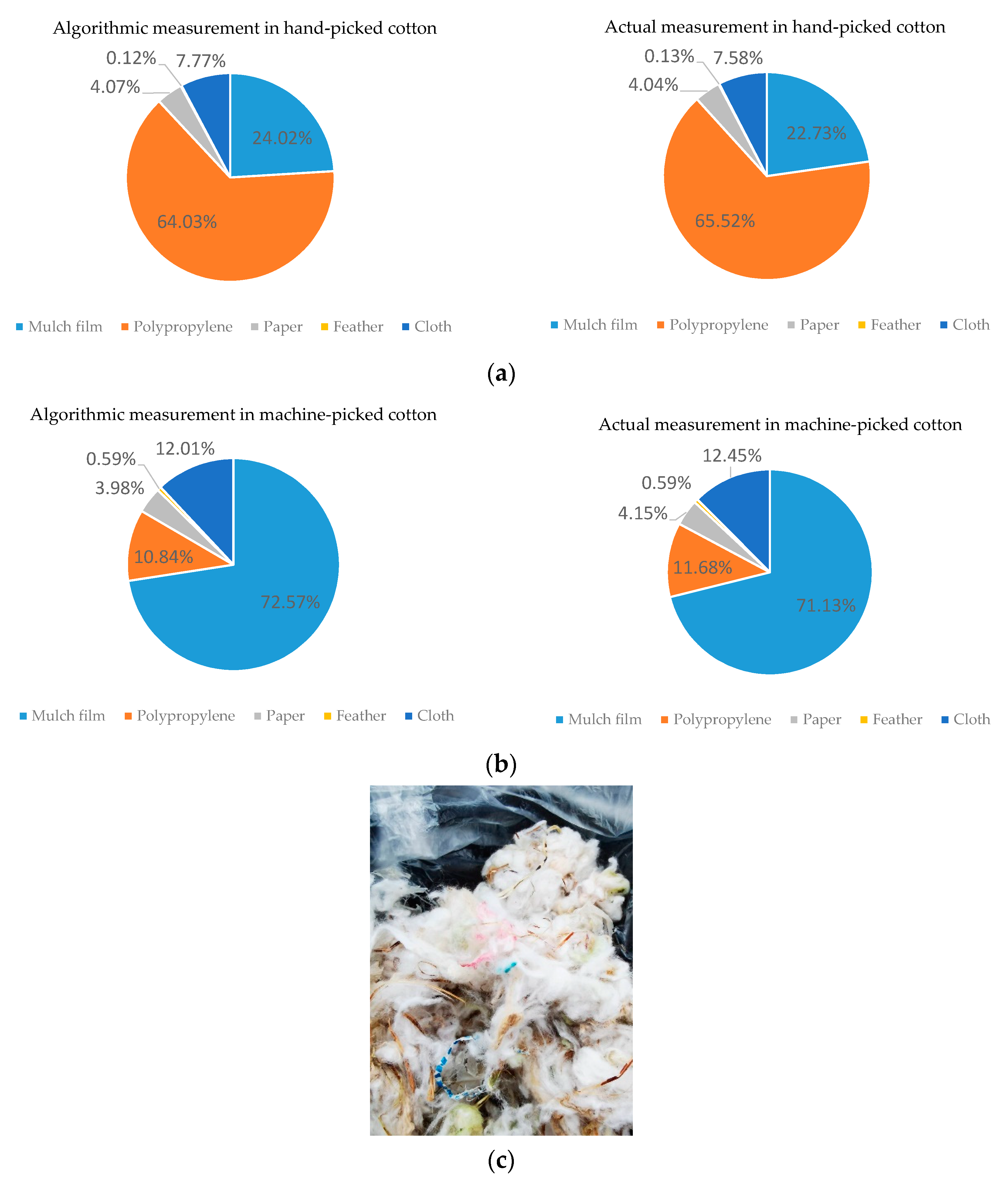
The practicability of the size evaluation algorithm was validated on the experimental prototype. The next step was to deploy the algorithm in different cotton mills for comparison. Two representative cotton mills were selected. One mainly used local hand-picked cotton, and its yarn products were used in curtains, garments, and other industries. The second one mainly used machine-picked cotton, and its products were mainly used in bedclothes.

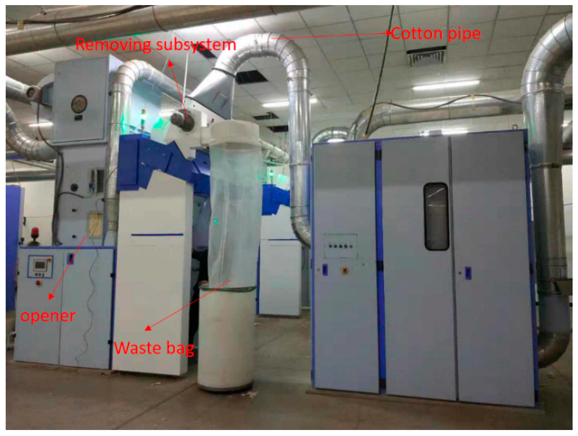
Hand-picked cotton often contains a lot of polypropylene, waste paper scraps, and other foreign fiber, which belongs to low-grade raw cotton. Machine-picked cotton is higher than hand-picked in the grade of raw cotton, but the machine-picked cotton is mainly covered by plastic film greenhouses, resulting in the introduction of more uncleaned mulch films. To save costs, many cotton mills mix two kinds of raw cotton. The actual production line is shown in Figure 14. The main function of the opener is to unfold the cotton layer so that foreign fiber can be fully exposed and the sorter can effectively capture the foreign fiber image, remove the foreign fiber through the removal mechanism, and collect it in the waste cotton bag. This paper randomly selected the estimation results of the statistical algorithm for time, and at the same time, it collected the foreign fiber in the corresponding time in the waste cotton bucket and detected the actual operation effect of the algorithm by comparing the size data.

The length of linear foreign fiber, such as polypropylene, is easy to measure, but for waste paper, animal feathers, mulch film, and another block foreign fiber, the area cannot be accurately calculated. However, foreign fiber content statistics are mainly used to estimate the grade of raw cotton and do not need a very precise value. Therefore, this paper estimated the area of block foreign fiber with an area meter and compared it with the results of the algorithm. The specific quantitative calculation method of foreign fiber size is shown in Figure 15. The length of the linear foreign fiber can be measured with a caliper, and the block foreign fiber can be estimated by an area meter. The measuring device was composed of a square 0.5 cm in length and width. If the foreign fiber occupied the square, the area could be considered as 0.25 square centimeters; if it was less than one grid, it could be rounded or roughly estimated.

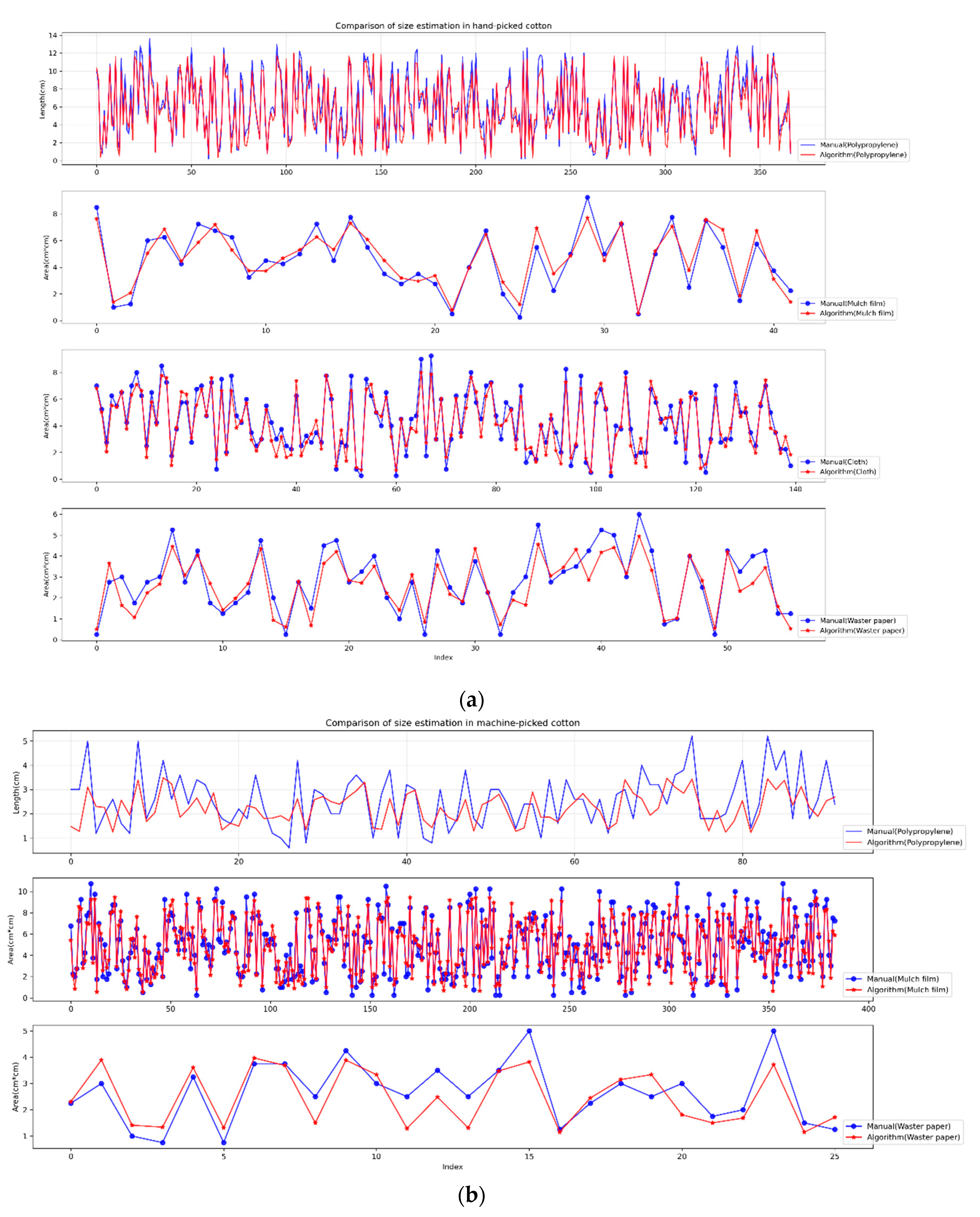
In two production lines with different types of raw cotton, two hours were randomly selected for comparison. The specific results are shown in

Table 8. The estimated size results of foreign fibers in a given time.

Class	Hand-Picked Cotton				Machine-Picked Cotton
	Count	Algorithm	Meter	RMSE	Count	Algorithm	Meter	RMSE
Mulch Film/cm2	42	191.8	196.5	0.78	384	1884.1	1910	0.91
Polypropylene/cm	367	2161.4	2327	0.98	92	207.2	238.2	0.82
Paper/cm2	56	610.2	587	0.75	26	64.3	68.8	0.7
Feather/cm2	1	2.57	2.5	-	3	10.192	10	-
Cloth/cm2	140	158.8	146.5	0.65	2	5.61	5	-

, as well as Figure 16 and Figure 17.

It can be seen from Table 8, and Figure 16 and Figure 17, that the size estimation after the algorithm segmentation had a good match with the real measurement. In the data comparison, we made statistics on the size of each sample, calculated the measurement difference between the corresponding samples, and then calculated the RMSE of the difference. It can be seen from the RMSE results that while the difference between the manual results and the algorithm was under 1, there were still errors in the content proportion between the algorithm and the actual size measurement, which mainly included the data method error of the actual measurement, the detection error of the foreign fiber machine, and the speed measurement error. However, the proportion of different fiber types is in line with the expectation. For example, in Figure 17a, the algorithm estimate that polypropylene accounted for was 65% in this time, which matched the overall proportion of actual measurement results and conformed to the characteristics of hand-picked cotton. Figure 17b belongs to the machine-picked cotton data, and mulch film accounted for more than 70%.

Since the foreign fiber cleaning machine cannot completely remove foreign fiber, much foreign fiber may be wrapped in the cotton, and false and missed detections may have existed in the system. In the actual situation, to reduce the omission of foreign fibers, some suspected foreign fibers that met the classification threshold were also classified as real foreign fibers, and size statistics were added. The overall size value calculated by the algorithm was generally greater than the actual value. As shown in Figure 18, the actual category was the cotton stalk, which belongs to pseudo fiber [34], but the classification probability returned by the classifier was 69% for polypropylene and 31% for the cotton stalk. After comprehensive consideration, it was still considered as polypropylene and was added into the statistics, resulting in a misjudgment from the real result.

6. Conclusions

This paper used an image segmentation algorithm based on deep learning to segment foreign fiber from the cotton, and then combined mechanical and camera parameters to implement a new method of foreign fiber content estimation on the foreign fiber cleaning machine. In terms of hardware, taking into account the application conditions and product costs, this article selected Nvidia’s Jetson-TX2 as the final algorithm realization platform. This platform could better adapt to the high-humidity, high-temperature, and high-dust environment of the cotton mill, and could accelerate the algorithm based on deep learning. We evaluated the main deep learning-based segmentation architectures, including FCN, U-Net, and SegNet. The test results on validation datasets showed that U-Net had the best performance in the most commonly used segmentation evaluation metrics, and the convergence speed of training loss was the fastest. In addition, on the JetsonTX2, the index recovery operation in SegNet could not use the acceleration function of the platform, and the operation time was the longest, while U-Net and FCN met the real-time operation requirement. Based on the result, we chose U-Net as the basic network architecture and, combined with the classification network, the results of the classifier were used as prior knowledge to train the decoder in U-Net. Experiments showed that the improved U-Net training convergence time was faster, and there was no need for separate classification time in the algorithm reasoning process, which saved the overall operation time of the system. Finally, the test of standard size samples on the experimental prototype showed that the RMSE of the estimated result and the actual size was 4% relative to the original size, and then the algorithm was deployed to different production lines. The distribution of estimated size and manually calibrated size in a random time was basically the same. Compared with the conventional sampling statistical method, it can provide more accurate evaluation data of the foreign fiber content of raw cotton.

In the follow-up research, the measurement method based on dynamic contour [35] can be used to measure the real foreign fiber area, make samples with objective and credible data, establish a mathematical model between the evaluation data and the actual data, and plan more refined report statistics. In addition, the cotton mills often evaluate foreign fiber content based on weight. The determination of foreign fiber weight through images is also the direction of the follow-up research, aiming to provide cotton mills with evaluation data of raw cotton foreign fiber content.