Entropy-Driven Adaptive Filtering for High-Accuracy and Resource-Efficient FPGA-Based Neural Network Systems

Abstract

Binarized neural networks are well suited for FPGA accelerators since their fine-grained architecture allows the creation of custom operators to support low-precision arithmetic operations, and the reduction in memory requirements means that all the network parameters can be stored in internal memory. Although good progress has been made to improve the accuracy of binarized networks, it can be significantly lower than networks where weights and activations have multi-bit precision. In this paper, we address this issue by adaptively choosing the number of frames used during inference, exploiting the high frame rates that binarized neural networks can achieve. We present a novel entropy-based adaptive filtering technique that improves accuracy by varying the system’s processing rate based on the entropy present in the neural network output. We focus on using real data captured with a standard camera rather than using standard datasets that do not realistically represent the artifacts in video stream content. The overall design has been prototyped on the Avnet Zedboard, which achieved 70.4% accuracy with a full processing pipeline from video capture to final classification output, which is 1.9 times better compared to the base static frame rate system. The main feature of the system is that while the classification rate averages a constant 30 fps, the real processing rate is dynamic and varies between 30 and 142 fps, adapting to the complexity of the data. The dynamic processing rate results in better efficiency that simply working at full frame rate while delivering high accuracy.

1. Introduction

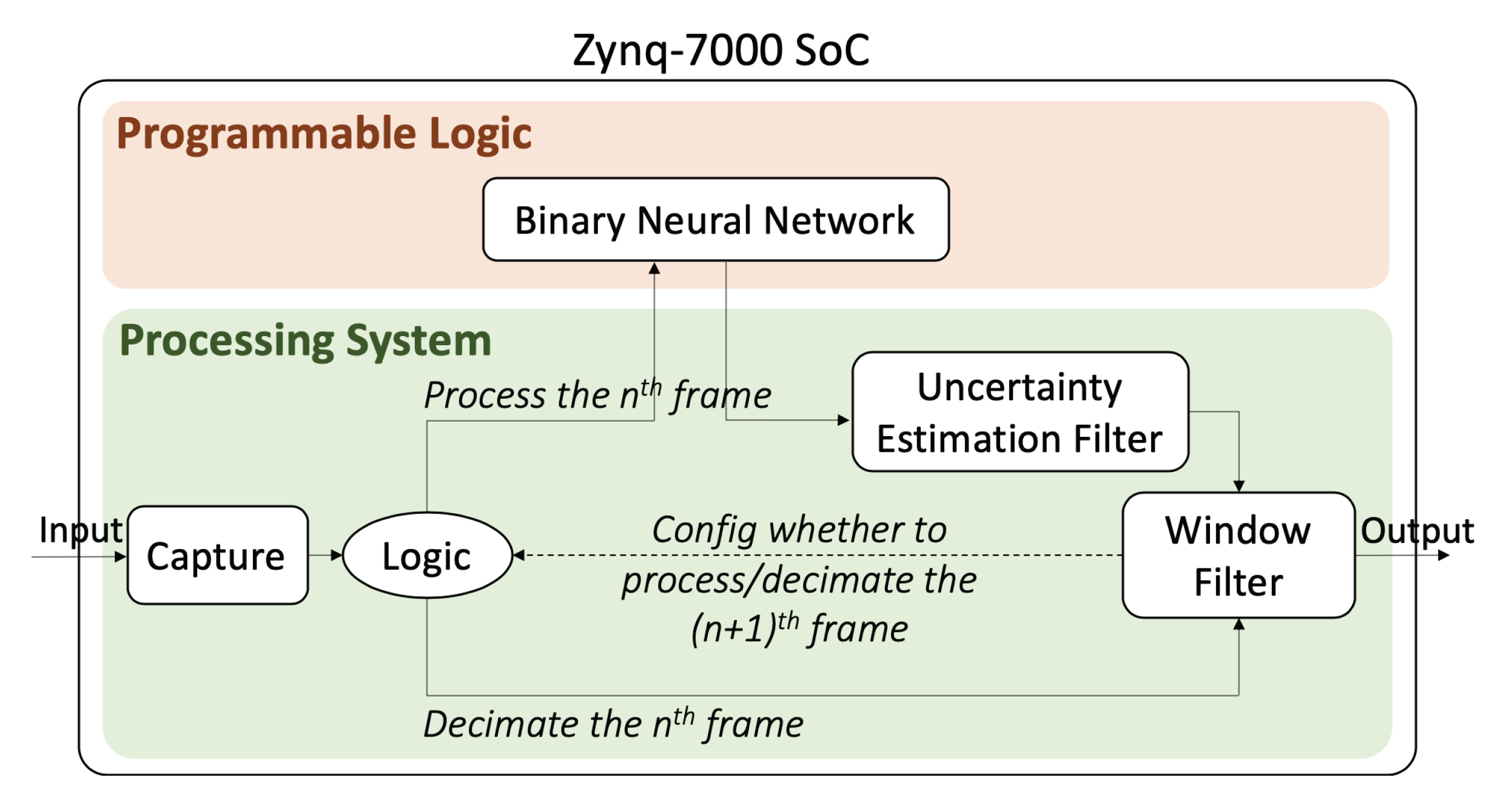
Neural networks running on general-purpose CPUs or GPUs are a common solution for image recognition problems, yet these solutions tend to be power-hungry or the level of performance falls below the requirements of many applications. Integer-precision neural networks deployed on FPGA accelerators have been shown to achieve very high performance per watt, although the level of accuracy can degrade significantly if the quantization process is done to binary levels, and hence they are more prone to prediction errors. To address this issue, we present a novel entropy-based adaptive filter, which is lightweight and modular. The overall system is shown in Figure 1. The inference part, which requires high parallelism, is executed on the programmable logic (PL), while the proposed filter is executed on the processing system (PS). The filter is used to improve the accuracy and adaptiveness of the system to variations in the input video. It mainly consists of a window filter and an uncertainty estimation filter. The processing pipeline works with real video frames instead of predefined datasets. It first improves the accuracy of the system by processing more frames in the background. Secondly, it estimates the confident level of the neural network model prediction. Finally, based on the confidence level, it decimates incoming frames or increases the number of frames being considered when computing the aggregated classification results. This is accomplished by changing the settings of the Window Filter.

The three main contributions of this paper are:

• We show how the accuracy of the low precision neural network working with real video data can be improved with increasing processing rates.
• We propose a novel entropy-based uncertainty estimation scheme and compared its performance with other estimation techniques.
• We created a novel neural network pipeline with software and hardware components that dynamically adjust the processing rate based on the uncertainty present in the neural network output.

Our end goal is to boost the real accuracy of low precision neural network systems and use adaptive schemes to adjust energy consumption dynamically based on data complexity.

2. Background and Related Work

FPGAs have become a popular choice with which to build neural network accelerators due to their programmability, high-performance and low-power consumption. FPGAs compete with custom architectures and GPUs [1] in this field, but current trends that favor sparse networks and compact data representation are well suited to the FPGA strengths. For example, accelerating binarized neural networks on FPGAs have several advantages, such as drastically reducing the required memory size and accesses during the forward-pass, and obtaining 2466 operations per the second of throughput, as most arithmetic operations can be replaced with bit-wise operations; for instance, Umuroglu [2] obtained a 2465.5 GOPS on CIFAR 10 dataset. Extreme compact data representation with binarized neural networks (BNNs) was introduced in [3] with single-bit neuron values and weights. These concepts were explored in hardware in [4]; the authors explored a BNN architecture. The binary implementations were obtained in FPGA, ASIC, CPU and GPU devices and showed significant acceleration compared with full precision, but the FPGA and ASIC alternatives outperformed CPU and GPU devices, which are limited by low device utilization—although the FPGA has a lower peak throughput than the GPU, it manages to use most of it. The comparison between FPGAs and ASIC showed, as expected, that performance/watt is one order of magnitude worse in the FPGA device but this value is reduced to 5× if only performance is considered. In this case, the advantage of the FPGA is its flexibility at creating new improved versions of the accelerator or adding other pre-processing blocks to the device, such as frame scaling, denoizing, etc., without the need for ASIC fabrication. A study of binary neural networks on device hybrids combining CPU + FPGA was performed in [5]. The study investigated which parts of the algorithm were better suited for FPGA and CPU implementation and considered both training and inference. The paper’s results were based on the hardware performance of the binarized matrix-matrix multiplication operator implemented with RTL and do not represent a full neural network. Results for the full network were extrapolated based on the analysis of a 10,240 × 10,240 × 10,240 matrix size multiplier. The considered Arria 10 FPGA device which had 1.1M logic cells achieved 40.7 TOPs at 312 MHz and power of 48 Watts. Routing congestion, buffering overheads between neuron layers and memory bandwidth limitations were not considered, since a full system was not proposed. A complete and efficient framework to implement BNNs on FFGA is FINN (a framework for fast, scalable binarised neural network inference)—[2]. FINN is based on the BNN method developed in [3], providing high performance and low memory cost using XNOR-popcount-threshold data-paths with all the parameters stored in on-chip memory. FINN has a streaming multi-layer pipeline architecture where every layer is composed of a computational engine surrounded by input/output buffers. A FINN engine implements the matrix-vector products of fully-connected layers or the matrix-matrix products of convolution operations. Each engine computes binarized products and then compares them against a threshold for binarized activation. It consists of P processing elements (PEs), each having S single instruction multiple data (SIMD) lanes. The first layer of the network receives non-binarized image inputs, and hence it requires regular operations, while the last layer outputs non-binarized classification results and does not require thresholding. The work presented in [6] used FINN to demonstrate a practical adaptive voltage scaling system called Elongate using the standard Zynq and Zynq Ultrascale FPGAs available in the zc702 and zcu102 boards, which are both equipped with programmable voltage regulators. It investigated the possible reductions in power with an adaptive voltage scaling system and the trade-offs between energy and performance. By scaling the voltage and frequency, Elongate obtained energy points that were up to 86% better than nominal at the same level of classification accuracy.

Binarized networks with FPGA accelerators can attain very high throughput, as demonstrated in BinaryEye [7]. The BinaryEye system also uses FINN and it adopts a pipeline approach in communication and processing: (a) conduct region-of-interest (ROI) extraction, binarize image with threshold function and classification with BNN; (b) buffer image at DRAM. The main difference between BinaryEye and our system is that we focus on adapting processing to real data instead of maximizing processing rate. Another very high throughput system is presented in [5], which achieved 40,770 GOPS by performing fine-grained partitioning on its Xeon + FPGA platform. Instead of sacrificing FPGA resources, the CPU can handle additional routing and configuration requirements in backpropagations. Furthermore, each layer can be staged, avoiding memory transfer overhead and utilizing the platform’s same address space properties, and inefficiency introduced by maintaining different address spaces is also mitigated.

Examples of floating-point neural network frameworks for FPGAs include DNNWEAVER [8], which shows that FPGA devices can deliver better performance-per-watt than GPUs and CPUs. DNNWEAVER generates synthesizable accelerators using a high-level specification in Caffe mapped to hardware templates written in Verilog code and is designed for floating-point precision.

From the previous work, it is clear that the extreme quantization in binarized networks results in very high performance, but the literature also indicates that it could be damaging to the accuracy of the network due to information losses. For example, FINN which is also adopted in this research, had a top-1 accuracy of 80.10% with 2465.5 GOPS on the CIFAR-10 dataset, but our analysis shows that, using the network with real data capture using a standard camera and outside of the standard CIFAR-10 dataset, accuracy can degrade significantly.

Compared with the presented previous work in this paper we focus on a system-level approach that exploits a heterogeneous architecture that contains CPU and FPGA computing resources. The neural network itself mapped to the FPGA uses the FINN library, and the software components built around it control this hardware accelerator by dynamically adjusting its throughput to improve overall system accuracy. The concept of working with a variable processing rate to avoid additional computing when not needed has been studied in related pieces of work. For example, BranchyNet [9] introduced the concept of early exit in neural network architecture to improve the efficiency of feedforward inference. It uses entropy to evaluate whether the classifier is confident in the prediction, and exits the network earlier when it gains enough confidence. BranchyNet trains a new network with multiple exit points by solving a joint optimization problem on the weight of the loss function associated with the exit points. The regularization effect of using multiple exit points prevents overfitting and helps to improve the overall accuracy. The branch locations are fixed and depend on the complexity of the dataset, which is not a problem with standard datasets but is unrealistic if real data is used. This approach was also investigated in [10] by Intel, which showed the benefits with Imagenet and CIFAR10 datasets. A more sophisticated approach to early exiting is presented in [11]; they used a network architecture with two dimensions, with network layers in the x dimension and multiple scale representations of the feature maps in the y dimension. This approach aims at improving the accuracy of early decisions by maintaining coarse and fine level features all-throughout the network. While also adopting similar principles, we do not modify the network architecture, since we do not aim at exiting earlier when we are certain about our prediction; instead, we change our filter parameters and decimate the next nth frames. Our filter applies to the overall system as an additional software module. This allows the filter to be adopted without retraining the neural network.

3. Methodology

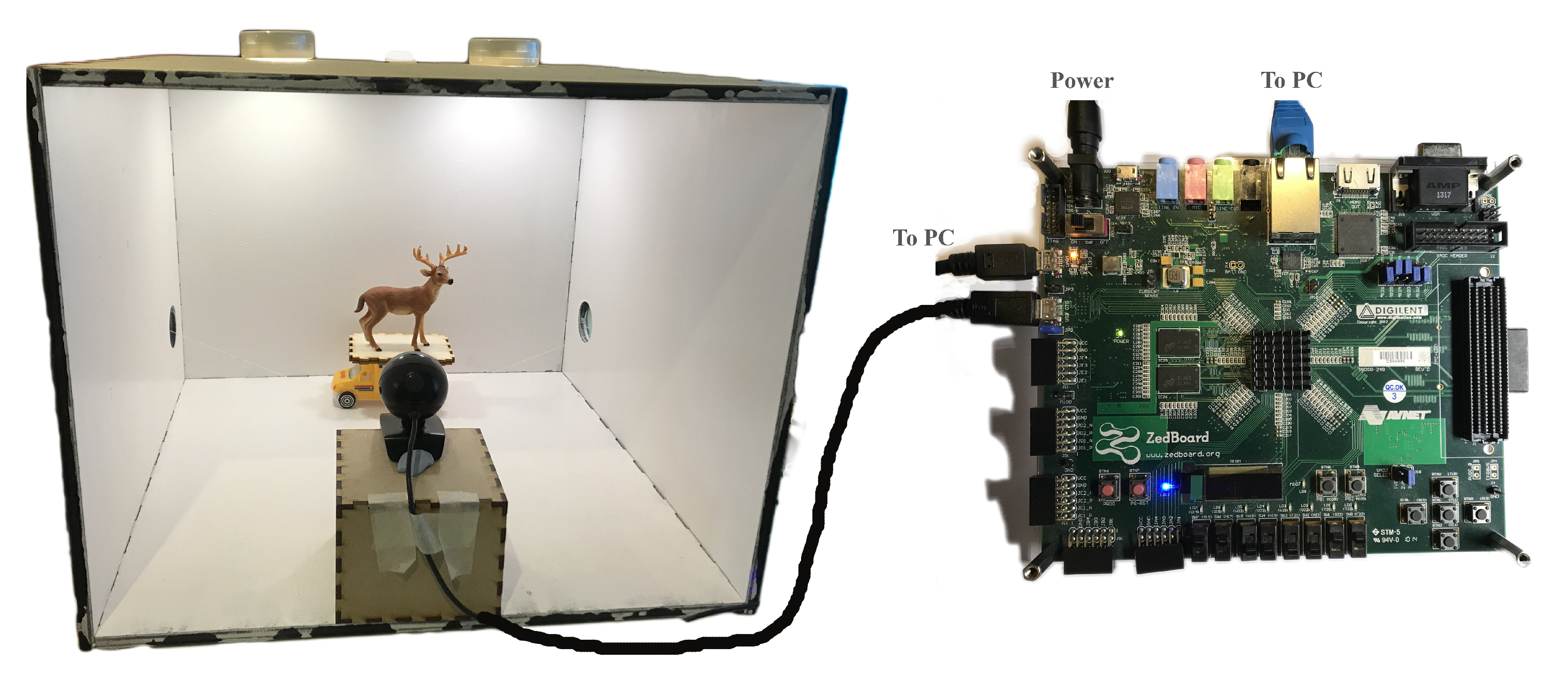
Our demonstrator is based on a low-cost Xilinx Zynq-7000 SoC ZedBoard and Logitech C160 webcam but it is fully compatible with larger or higher-performance FPGAs from other families, such as Zynq Ultrascale, as long as CPU and FPGA resources are available. The use of low-cost FPGA and low-cost sensor enables the development of cost-effective solutions that are suitable for industrial and commercial applications. The image sensor is tuned to a low-resolution setting (320 × 240) to provide a higher frame rate at ≅160 fps. This enables a processing dynamic range between 30 and 160 fps. The Zynq-7000 Cortex A9 processors can run a fully-featured Ubuntu OS so video processing libraries such as OpenCV are available for ease of development. The FINN network was mapped to the FPGA part of the Zynq-7020 device with a clock of 100 MHz and the complexity results are shown in

Table 1. BNN implementation utilization report on Zynq-7000.

LUTs	FFs	DSPs	BRAMs
25,980 (49%)	36,115 (34%)	32 (15%)	132 (94%)

with the percentage of used device in brackets. Table 1 shows that due to memory limitations larger networks cannot be supported in this device.

The network has been trained with the CIFAR-10 dataset and the output of the BNN is a 1-D array of size 10. This 1-D array represents how likely the input from each of the classes (aeroplane, automobile, bird, cat, deer, dog, frog, horse, ship, truck) is, and it is often referred to as the class scores array. Moreover, the FINN network takes as input images with 32 × 32 pixels, so the output from the webcam needs to be downsampled before passing it to the BNN for inference.

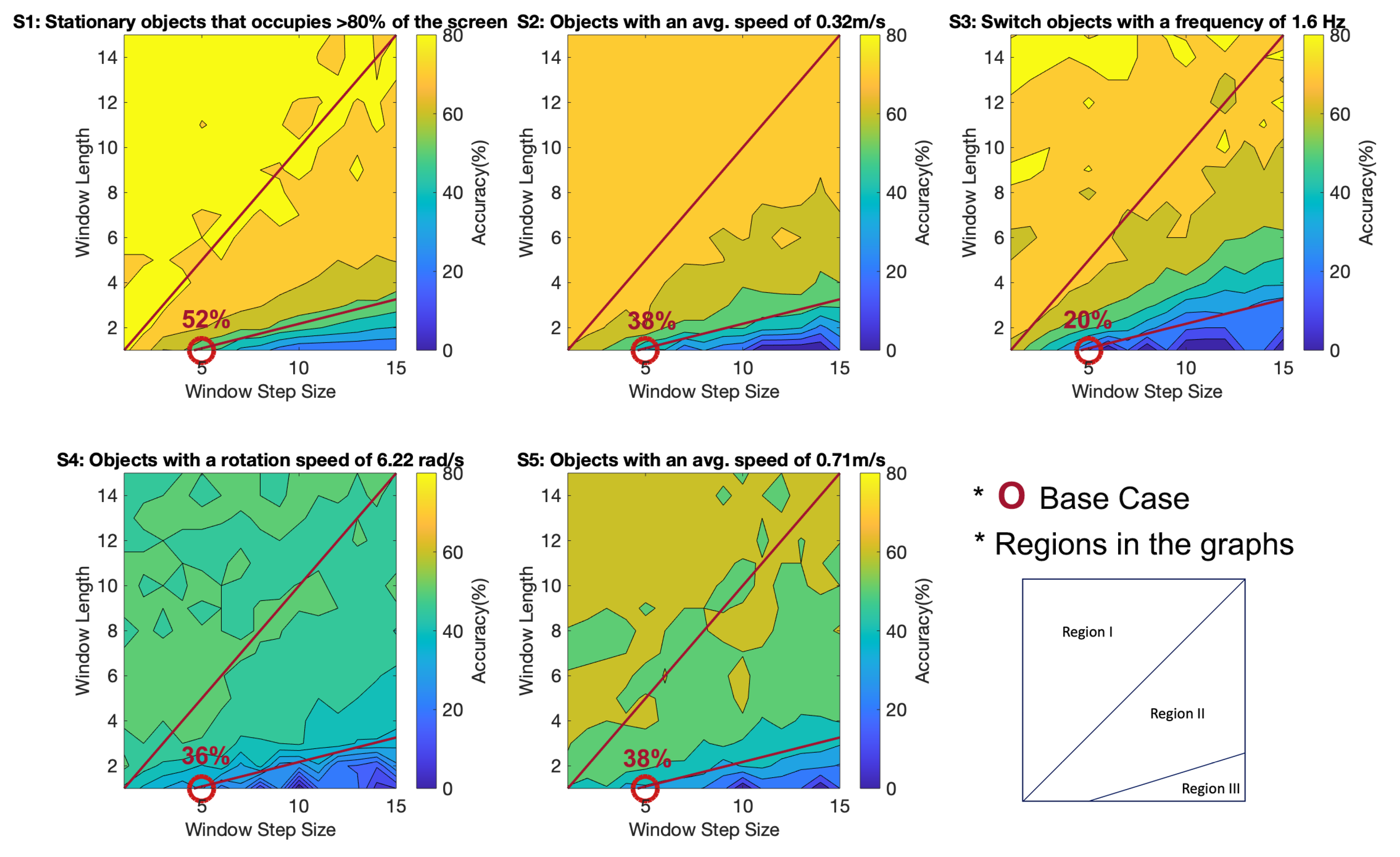
To evaluate the performance of the system with real data and in a consistent setting, a constant lighting box was built and five video datasets (S1–S5) have been generated with the control setup, as shown in Figure 2 to evaluate the impacts of object size, speed and orientation on classification accuracy. S1–S5 are: stationary objects that occupy $>80$ of the screen, objects with an average speed of 0.32 m/s, switch objects with a frequency of 1.6 Hz instead of 0.8 Hz, objects with a rotation speed of 6.22 rad/s and objects with an average speed of 0.71 m/s. Furthermore, U1–U4 have been set up to evaluate the uncertainty estimation schemes in face of changes. They combine frames from dataset 1 with datasets 2–5 respectively, and the point of change was digitally controlled at frame number 100. This allowed us to analyze the performances of various uncertainty estimation schemes at the point of change. More details of the datasets can be found in

Table 2. Details of self-generated datasets.

	No. of Frames				Occasionally
Datasets	per Object	Obj. Size	Obj. Speed	Rotating	out of Frame	Properties
S1	200 (0.8 Hz)	80%	0 m/s	0 rad/s	No	Stationary and Large object size
S2	200 (0.8 Hz)	50%	0.32 m/s	0 rad/s	No	Slow Motion
S3	100 (1.6 Hz)	50%	0.32 m/s	0 rad/s	No	High Switching Frequency
S4	200 (0.8 Hz)	50%	0.32 m/s	6.22 rad/s	No	Rotating
S5	200 (0.8 Hz)	50%	0.71 m/s	0 rad/s	Yes	Fast Motion
U1	Object motion changes from stationary to 0.32 m/s (S1 to S2)
U2	Object switching frequency changes from 0.8 Hz to 1.6 Hz (S1 to S3)
U3	Object rotational speed changes from 0 rad/s to 6.22 rad/s (S1 to S4)
U4	Object motion changes from stationary to 0.71 m/s (S1 to S5)

U1–4 datasets combine frames from dataset 1 and datasets 2–5 respectively, where the point of change is at frame number 100.

.

4. Proposed Window Filter

A window filter is commonly used in stream data processing to compute aggregates over bounded subsets of a stream, called a window. Outputting the aggregated classification results over the instantaneous ones allows us to combat random noise introduced by the image sensor and take into account previous classification results.

In terms of the window filter’s parameters, window length $l_{WL}$ specifies how many past instantaneous classification results are considered, while window step size $l_{SS}$ specifies how frequently the aggregated classification result is computed. Current and past BNN outputs (class scores arrays) are multiplied with the the filter weights and summed together to generate the final aggregated result. To suit our use case, an exponential decay aggregation function has been adopted, with the most recent results having the heaviest weights.

Weights of filter with window length $l_w$:

$$\begin{array}{cc}\hfill {\overrightarrow{W}}^T& =\left[\begin{array}{ccccc}{e}^0& e^{-\lambda }& e^{-2\lambda }& \cdots & e^{-\lambda (l_w-1)}\end{array}\right]\hfill \end{array}$$

A ($l_w$× 10) matrix $\mathbf{D}$ has been used to store recent class scores array, with ${\mathbf{D}}_{\mathbf{0}\mathbf{j}}$ being the class scores of the current frame.

The product of the weights and the data gives the aggregated result $\overrightarrow{AD}$:

$$\begin{array}{cc}\hfill \overrightarrow{AD}& ={\overrightarrow{W}}^T\times \mathbf{D}\hfill \end{array}$$

Finally, the adjusted output would be the class with the highest score in $\overrightarrow{AD}$.

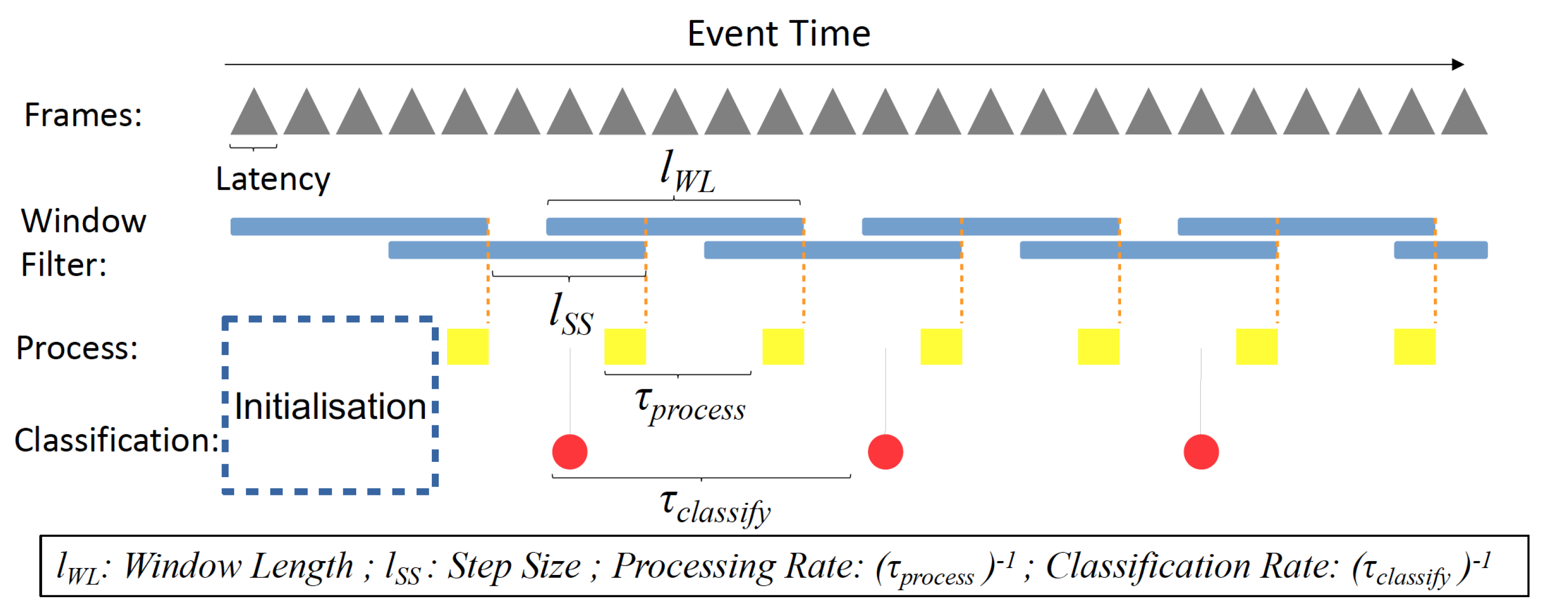
In this paper, we add an additional layer of abstraction on top of the usual window filter. Thanks to the extremely fast inference speed provided by FINN, we have margins to differentiate between a required user classification rate (set arbitrarily at 30 fps), the internal processing rate (> 30 fps and < 160 fps) and the camera frame rate (160 fps). The window filter is part of the internal processing and aggregated results are extracted for display purposes at a slower rate (referred to as classification rate).

As illustrated in Figure 3, in each yellow square, the aggregate will be recomputed, and the internal classification will be updated. At every red circle, on-screen classification labels will be updated with the current internal classification labels.

The different rates are being defined as follows:

$$\begin{array}{cc}\hfill \mathit{Latency}& =\mathit{Avg}. \mathit{Time} \mathit{Taken} \mathit{to} \mathit{Capture} \mathit{and} \mathit{Classify} \mathit{an} \mathit{Image}\hfill \end{array}$$

(1)

$$\begin{array}{cc}\hfill \mathit{Processing} \mathit{Rate}& =\frac{\mathit{No}. \mathit{of} \mathit{Frames} \mathit{Processed} \mathit{by} \mathit{Hardware} \mathit{Functions}}{\mathit{Total} \mathit{Latency}}={\left({\tau }_{process}\right)}^{-1}\hfill \end{array}$$

(2)

$$\begin{array}{cc}\hfill \mathit{Classification} \mathit{Rate}& =\frac{\mathit{No}. \mathit{of} \mathit{times} \mathit{classification} \mathit{labels} \mathit{being} \mathit{updated}}{\mathit{Total} \mathit{Latency}}={\left({\tau }_{classify}\right)}^{-1}\hfill \end{array}$$

(3)

5. Baseline and Regions Definition

To update the classification labels at an approximately 30 fps base rate to the user and with a camera frame rate of 160 fps camera frame rate, we set a baseline model with a window filter step size of 5 (160/30 ≈ 5). Furthermore, as a baseline, no aggregation functions are applied on it; therefore, it has a window filter length of 1. (Therefore, in experiments, window filter with 5–1 setting (step size = 5, length = 1) has been used for baseline). Hence, the base model is equivalent to a 30 fps basic classification system without any aggregation functions. Furthermore, as the number of frames being processed equals to the number of times classification labels being updated, according to Equations (2) and (3), the classification rate is identical to the processing rate in the base model. We will use this baseline system as the reference we want to improve accuracy on.

Additionally, to analyze the performances of different window filter step sizes and length combinations, we divide the step size and window length grid into three regions. Region I is where no frames are decimated, i.e., points where window length is larger than step size.

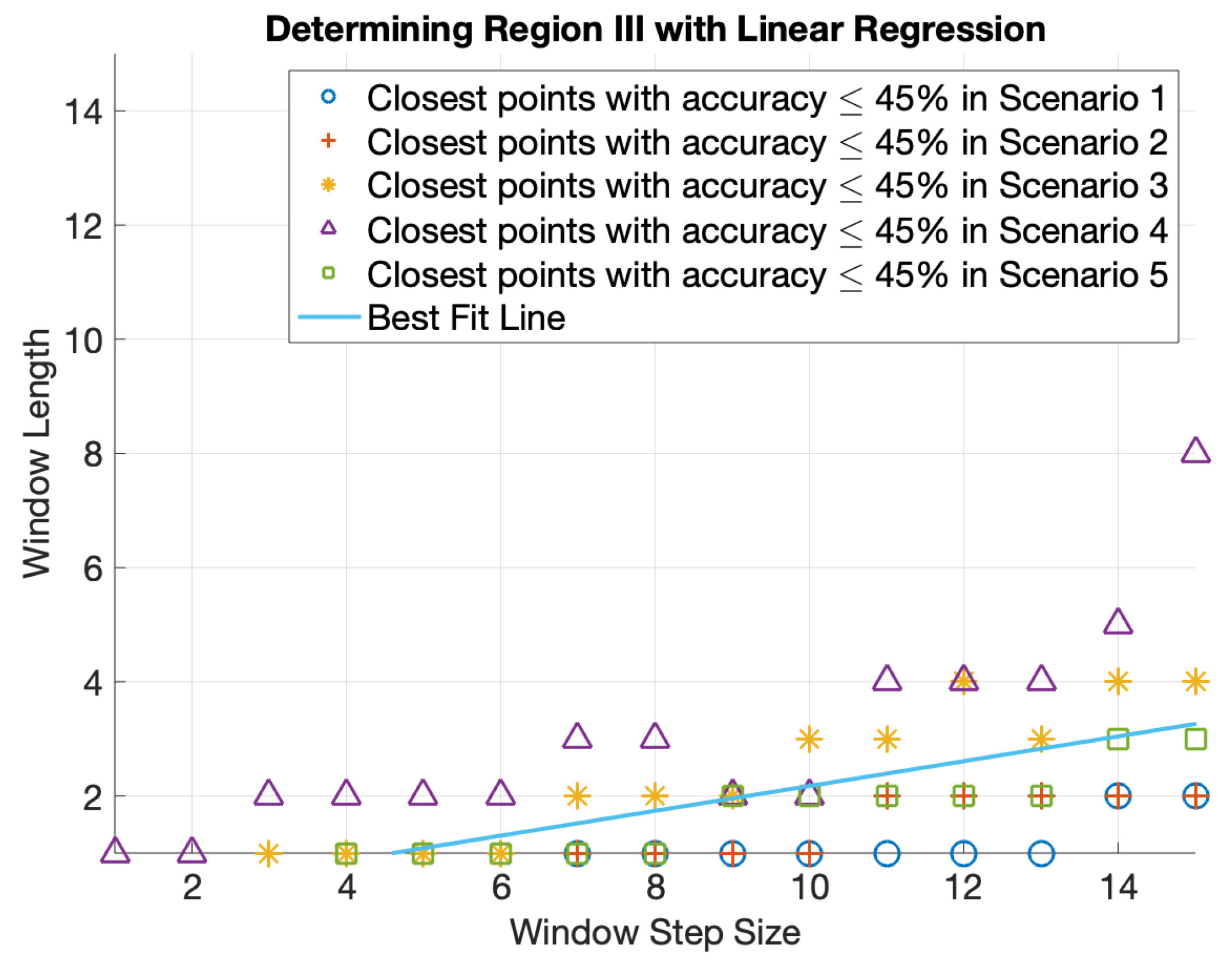
In areas where frames are being decimated (i.e., window step size > window length), it is noticeable that there is a particularly low accuracy region (dark blue) at the bottom right corner in all five scenarios. Therefore, we define an additional region III, to avoid using configurations from those areas. Considering the accuracy ranges of various scenarios, 45% accuracy has been chosen as an accuracy threshold to identify region III. To define the boundary of region III, we extract the closest points with accuracy less than or equal to 45% in all scenarios as shown in Figure 4. Then, the best fit line has been determined by applying a linear regression model on the data points. Region III would be the points on the bottom right of the best fit line.

6. Window Filter Evaluation

Accuracy results for the different video streams and window filter configurations have been shown in Figure 5. This experiment aimed to prove that window filters with appropriate configurations can improve the system’s accuracy. Furthermore, it was hoped that general trends in classification accuracy vs. window filter configurations could be identified, and optimum filter configurations could be found.

The first observation is: in Figure 5, the yellow regions show higher accuracy than blue. The figure shows that a large window length and a small step size (region I) result in relatively higher accuracy in all scenarios, while a large step size and a short window length (region II) tend to result in poor accuracy performance in all scenarios. The decline in accuracy could be explained that when the step size is larger than the window length (regions II and III), the system decimates frames, as calculated in Equation (4). Additionally, this often results in poor accuracy due to information loses. Although decimating frames often results in lower accuracy, that decreases the total number of processed frames equivalent to a lower processing rate, as indicated in Equation (2). This helps save computational resources. Therefore, if efficiency is also one of the goals, region II could be used to achieve high accuracy while reducing processing, and this is especially true for the case of stationary objects that occupy $>80\%$ of the screen, objects with an average speed of 0.32 m/s and switch objects with a frequency of 1.6 Hz.

$$\mathit{No}. \mathit{of} \mathit{frames} \mathit{decimated} \mathit{per} \mathit{cycle}=\mathit{Window} \mathit{Step} \mathit{Size}-\mathit{Window} \mathit{Length}$$

(4)

The second observation is that there is also a particularly low accuracy region in all scenarios—region III—which comprise points with extremely short window lengths. Our baseline lies in that region as well, with an average accuracy of 36.8%. This helps to prove our hypothesis that by considering more frames (using window filter with longer window length) the system accuracy can be improved.

Thirdly, the rotating object (S4) and fast motion (S5) cases tend to have overall lower accuracy performances compared to the other video types. This could be explained as the result of a change in the object’s orientation and speed that could block or blur the object prominent features that the network relies on for accurate classifications.

Overall, we observed that window filters with appropriate configurations can improve the system’s accuracy. It is also clear that different window filter settings are preferred under different scenarios to optimize system accuracy. Based on the above findings, we have identified five window filter settings with the highest accuracy in each region–scenario pairs as listed in

Table 3. Window filter configurations with highest accuracy for each region–scenario pair according to Figure 5 (notation: ${\ell }_{SS}$ = step size, ${\ell }_{WL}$ = window length).

	Region 1			Region 2			Region 3
Scenario	Step Size	Win. Length	Acc.(%)	Step Size	Win. Length	Acc.(%)	Step Size	Win. Length	Acc.(%)
S1: Stationary objects	2	11	85.0	10	9	83.5	14	3	58.0
that occupies > 80%	10	13	85.0	10	10	83.5	15	3	54.5
of the screen	10	14	85.0	11	11	83.0	10	2	54.0
S2: Objects with an	10	15	80.0	15	15	78.5	14	3	51.5
average speed	1	15	79.0	10	10	78.0	15	3	51.5
of 0.32 m/s	5	15	79.0	10	8	77.5	10	2	51.0
S3: Switch objects with	12	15	89.0	15	12	85.0	14	3	27.0
a frequency of 1.6Hz	1	14	86.0	12	10	84.0	15	3	24.0
instead of 0.8 Hz	2	14	86.0	15	14	82.0	10	2	22.0
S4: Objects with a	1	10	53.0	15	10	52.5	14	3	39.5
rotation speed	5	10	53.0	5	4	51.5	15	3	36.5
of 6.22 rad/s	2	5	52.5	7	7	51.5	5	1	36.0
S5: Objects with an	10	13	66.0	10	8	67.0	14	3	44.5
average speed	11	15	64.5	13	13	63.5	11	2	42.0
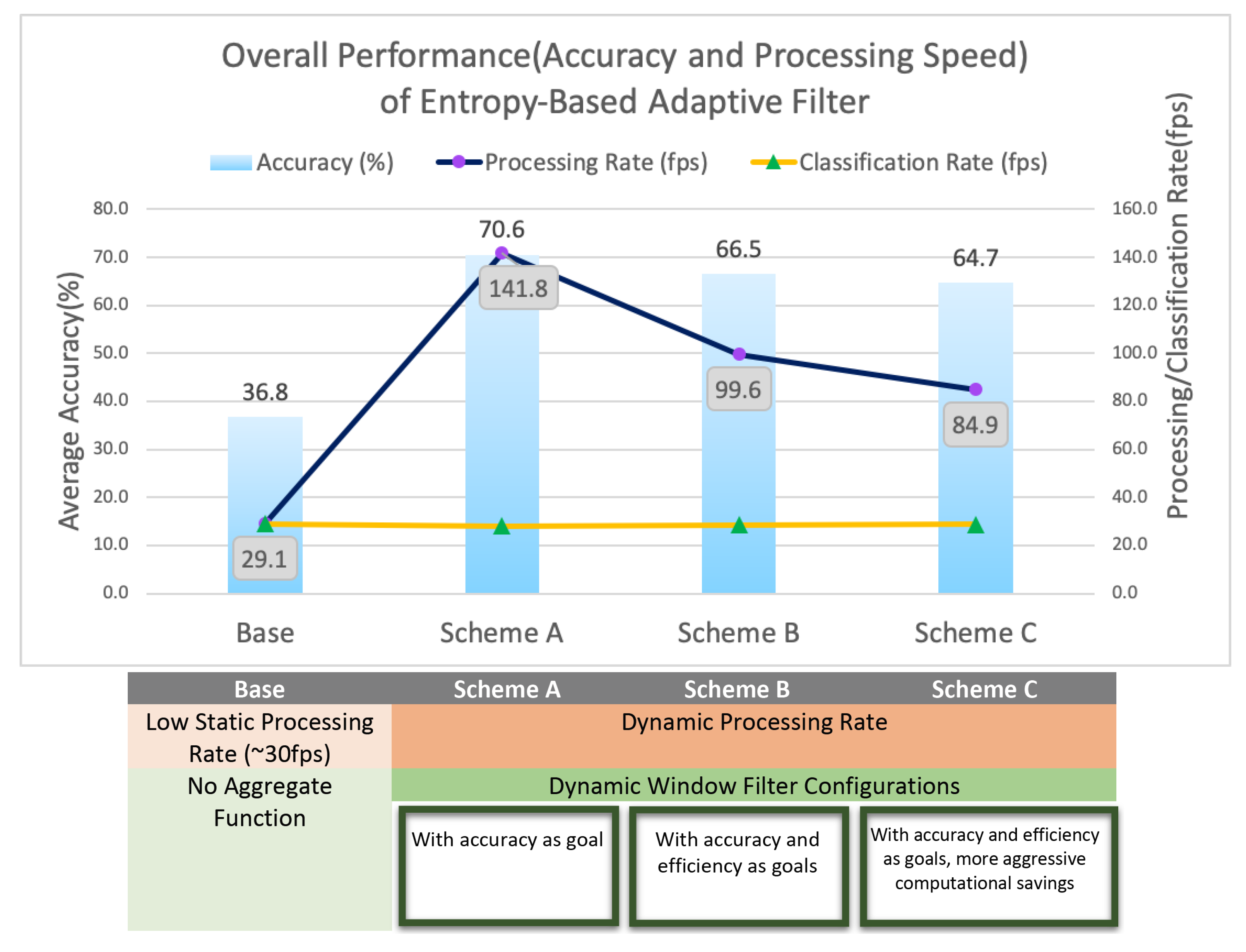
of 0.71 m/s	1	11	64.0	15	13	63.5	10	2	41.0

. The reason to separate them into regions was to allow us to analyze further the relations between system accuracy and efficiency. Then, for performance evaluation purposes, we chose three lists of optimal window filter configurations: scheme A for optimizing accuracy only; and schemes B and C for optimizing accuracy and efficiency. The difference between schemes B and C lies in that C decimates more frames, providing a set of more aggressive processing saving configurations. Each scheme comprises five window filter configurations, which correspond to the four scenarios (S2–S5) and the initialization stage. For the initialization stage, 1-one window filter configuration was used to ensure the system was properly set up.

Window filter configurations were chosen based on the rules defined below:

• Scheme A with accuracy as the goal: adopted window filter settings with highest accuracy from Table 3 region I.
• Scheme B with accuracy and efficiency as goals: adopted window filter settings with highest accuracy from Table 3 region II.
• Scheme C with accuracy and efficiency as goals (with more aggressive computational savings): adopted window filter settings with most frames decimated from Table 3 region II.

This helps us formulated

Table 4. Recommended window filter configurations based on the rules defined (window step size–window length).

Scenarios	Scheme A	Scheme B	Scheme C
Initialization	1–1	1–1	1–1
S2	10–15	15-15	10–8
S3	12–15	15–12	15–12
S4	1–10	15–10	15–10
S5	10–13	10–8	10–6

Scheme A: Optimized for accuracy only; scheme B: Optimized for accuracy and efficiency; scheme C: Optimized for accuracy and efficiency; more aggressive computational savings.

. And in the next section, we explore how to use the level of uncertainty in the neural network output as an indicator of which scenario the external environment is most likely to be at. Then, we will change the window filter settings dynamically based on the identified scenarios.

7. Proposed Uncertainty Estimation Measures

The uncertainty present in the BNN output could be a useful indicator of the external environment, as the class scores array obtained at the end of the pipeline and predictive probabilities (SoftMax output) could be interpreted as model confidence. Using this estimation of the external environment, frames could be decimated when the situation allows it—creating an adaptive system with a dynamic processing rate. This approach should result in overall better accuracy and energy efficiency since additional processing is only done when it is required.

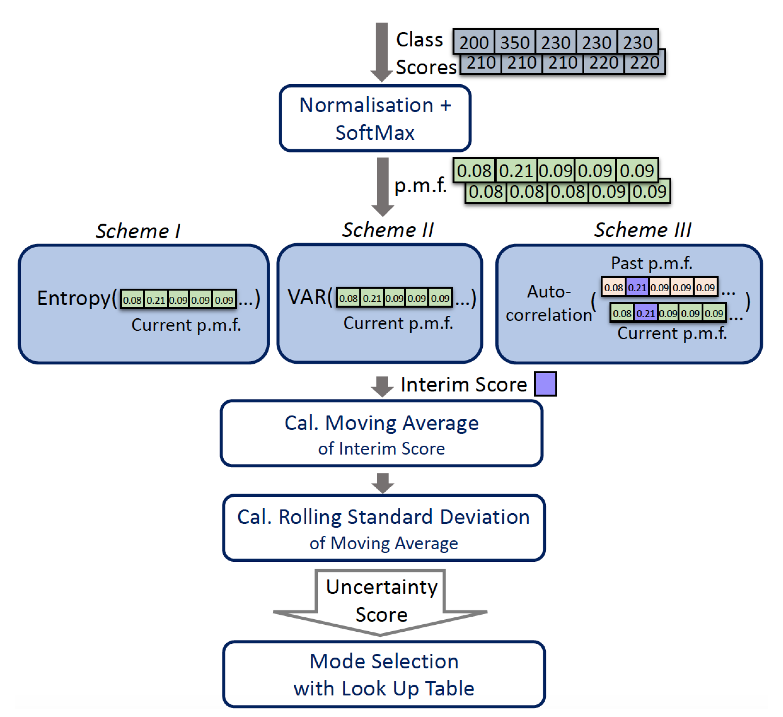
We evaluated three possible schemes to estimate uncertainty: entropy, variance and autocorrelation were used to calculate uncertainty scores. The overall uncertainty estimation pipeline is shown in Figure 6. At the end of the neural network pipeline, a class score $\overrightarrow{A^{t0}}$ array will be obtained, which represents how likely the input is from each class. By normalizing and applying the softmax function on the array, we can obtain the probability mass function (p.m.f.) $\overrightarrow{B^{t0}}$.

$$\mathbf{A}=\left(\begin{array}{c}{\overrightarrow{A}}^{t0}\\ {\overrightarrow{A}}^{t1}\\ {\overrightarrow{A}}^{t2}\\ ⋮\end{array}\right)=\left(\begin{array}{cccc}{a}_0^{t0}& a_1^{t0}& \cdots & a_9^{t0}\\ a_0^{t1}& \cdots \\ ⋮& \ddots \\ a_0^{tk}& & & a_9^{tk}\end{array}\right) \mathbf{B}=\left(\begin{array}{cccc}{P}_A\left(a_0^{t0}\right)& P_A\left(a_1^{t0}\right)& \cdots & P_A\left(a_9^{t0}\right)\\ P_A\left(a_0^{t1}\right)& \cdots \\ ⋮& \ddots \\ P_A\left(a_0^{tk}\right)& & & P_A\left(a_9^{tk}\right)\end{array}\right)=\left(\begin{array}{c}{\overrightarrow{B}}^{t0}\\ {\overrightarrow{B}}^{t1}\\ {\overrightarrow{B}}^{t2}\\ ⋮\end{array}\right)$$

These predictive probabilities can be passed to one of three uncertainty estimation schemes to obtain a floating-point number as an interim score. Both entropy and VAR treat input data at different timestamps as independent events, and hence only require the current p.m.f. $\overrightarrow{B^{t0}}$, while autocorrelation considers the temporal dependency between data points and estimates how correlated the current input is to the previous data; hence, it also requires past p.m.f. ($\overrightarrow{B^{t1}}$, $\overrightarrow{B^{t2}}$, $\overrightarrow{B^{t3}}\cdots$). Additionally, the autocorrelation operation will generate a 1-D array of size 10, representing the correlation of each class score with its predecessors. Only the correlation index relevant to the output classes is selected as the interim score.

The moving average of the interim score is then updated with the rolling mean equation (Equation (5)). ${\overline{x}}_0$ and ${\overline{x}}_1$ denote the sample means of $x_0\dots x_{k-1}$ and $x_1\dots x_k$ respectively, with $x_k$ being the oldest sample.

$${\overline{x}}_0={\overline{x}}_1+\frac{x_0-x_k}{k}$$

(5)

This reduces the update time complexity from O(k) to O(1), compared to standard mean calculation. The averaging function can be viewed as a low pass filter to smooth out short-term fluctuations and highlight long-term trends. Changes in the long-term trends are then quantified with variance statistics.

The rolling standard deviation of the most recent k moving average of interim scores can be updated with Welford’s algorithm [12], a single-pass method that alleviates the prohibitive computation overhead of a two pass method. [13] $M_0$ and $M_1$ denotes the current and previous aggregated sums (in standard deviation equations).

$$\begin{array}{cc}\hfill M_0=M_1& +(x_0-{\overline{x}}_0)\times (x_0-{\overline{x}}_1)\hfill \\ \hfill & -(x_k-{\overline{x}}_0)\times (x_k-{\overline{x}}_1)\hfill \end{array}$$

(6)

Finally, the sample standard deviation ${\sigma }_0$ was obtained via Equation (7), where k equals the number of data points we are considering.

$${\sigma }_0=\sqrt{\frac{M_0}{k-1}}$$

(7)

The standard deviation is our final uncertainty score. It will be compared to a lookup table to determine the level of uncertainty and which scenario we are in.

7.1. Scheme I: Entropy

From the perspective of information theory, we can view the system as a general communication channel. The Shannon entropy allows us to quantify the average level of "surprise" (uncertainty) inherent in the probability distribution of the outcome. Given the output of the BNN with 10 possible outcomes, and the probability that the input belongs to a certain class represented by SoftMax output ${\overrightarrow{B}}^{t0}={\overrightarrow{P}}_{A^{t0}}$, Shannon entropy H can be calculated as follows with i representing different classes:

$$\mathit{interim} \mathit{score}=H\left({\overrightarrow{A}}^{t0}\right)=-\sum _{i=0}^9{P}_A\left(a_i^{t0}\right){log}_2{P}_A\left(a_i^{t0}\right)$$

(8)

Entropy is maximized at the uniform distribution, as the channel’s outcome does not indicate which event is more likely to happen, and hence, it is the most uncertain case. It is minimized when there is a 100% probability of a certain event happening, which is the most certain case.

7.2. Scheme II: VAR

VAR (variance) is used to measure how "spiky" the probability distribution is. If the p.m.f. from SoftMax calculation has a high variance (flat distribution), it implies that the classifier interprets that the input contains a lot features from multiple classes, which indicates a higher uncertainty scenario. On the other hand, if the resultant p.m.f. has a low variance (spiky distribution), it implies that the classifier predicts that the input belongs to a single class, and is more confident of its prediction. This concept is very similar to entropy, and their performance and complexity will be evaluated in the next section. Let $b_i^{t0}$ be the predictive probabilities in ${\overrightarrow{B}}^{t0}$ that correspond to each classes and $\overline{b}$ be the mean of ${\overrightarrow{B}}^{t0}$. (Note that $b_i^{t0}$ equivalent to $P_A\left(a_i^{t0}\right)$). The variance ${\sigma }_{t0}^2$ is:

$$\mathit{interim} \mathit{score}={\sigma }_{t0}^2=\frac{\sum \left(b_i^{t0}\right)\overline{b}{)}^2}{10-1}$$

(9)

The variance of the p.m.f. is then output as the interim score.

7.3. Scheme III: Autocorrelation

Finally, the time series can also be interpreted as a weakly-stationary stochastic process, where stochastic process refers to a random processes and stationary refers to processes whose unconditional joint probability distribution is invariant of shifts in time. We can view the data as repeated measurements from the image sensor. We assume that the p.m.f. of the outcome remains constant within a short period, and hence, weakly stationary. Observations collected at different times are dependent on each other. This temporal dependence feature implies that the common assumption of independence no longer holds. Therefore, we can also specify the statistical uncertainty through the autocorrelation, taking reference from the paper, "Using the autocorrelation function to characterize time series of voltage measurements" [14]. This allows us to take into account dependency among data.

The previous methods only considered the current p.m.f. ${\overrightarrow{B}}^{t0}$; however, given that measurements taken with the image sensor are also a weakly-stationary stochastic process, we can consider more historical data (${\overrightarrow{B}}^{t1}$, ${\overrightarrow{B}}^{t2}$, ${\overrightarrow{B}}^{t3}\cdots$) to utilize the temporal correlation among measurements. Autocorrelation is the correlation of a signal with a delayed copy of itself as a function of delay, and similarity between observations can then be inferred from it. If the current sensor signal is very similar to the previous one, that shows the external environment is stable. Hence, the level of certainty is high. Otherwise, if the measurements’ discrepancy is high, this shows the environment is changing, and hence less certain.

Let autocorrelation with lag k be $\overrightarrow{R}(t0,tk)=[r_1(t0,tk),r_2(t0,tk)\cdots r_{10}(t0,tk)]$ and i representing different classes.

$$\begin{array}{c}\begin{array}{c}\hfill r_i(t0,tk)=E_i\{{\overrightarrow{B}}_i^{t0},\overrightarrow{B}{*}_i^{tk}\}=\frac{b_i^{t0}\times b_i^{t1}+b_i^{t1}\times b_i^{t2}\cdots +b_i^{tk-1}\times b_i^{tk}}{k}\end{array}\end{array}$$

(10)

To reduce time complexity, we have also derived an update rule from definitions for rolling autocorrelation as shown below.

$$r_i(t0,tk)=R_i(t1,tk+1)+\frac{(b_i^{t0}\times b_i^{t1})-(b_i^{tk}\times b_i^{tk+1})}{k}$$

The object in frame is predicted to be the classes with the maximum scores $A^{t0}$. Hence, we define the interim score as:

$$\begin{array}{cc}\hfill \mathit{output}& =\mathit{position} \mathit{of} max\left(\overrightarrow{A^{t0}}\right)\hfill \\ \hfill \mathit{interim} \mathit{score}& =r_{output}^{t0}\hfill \end{array}$$

(11)

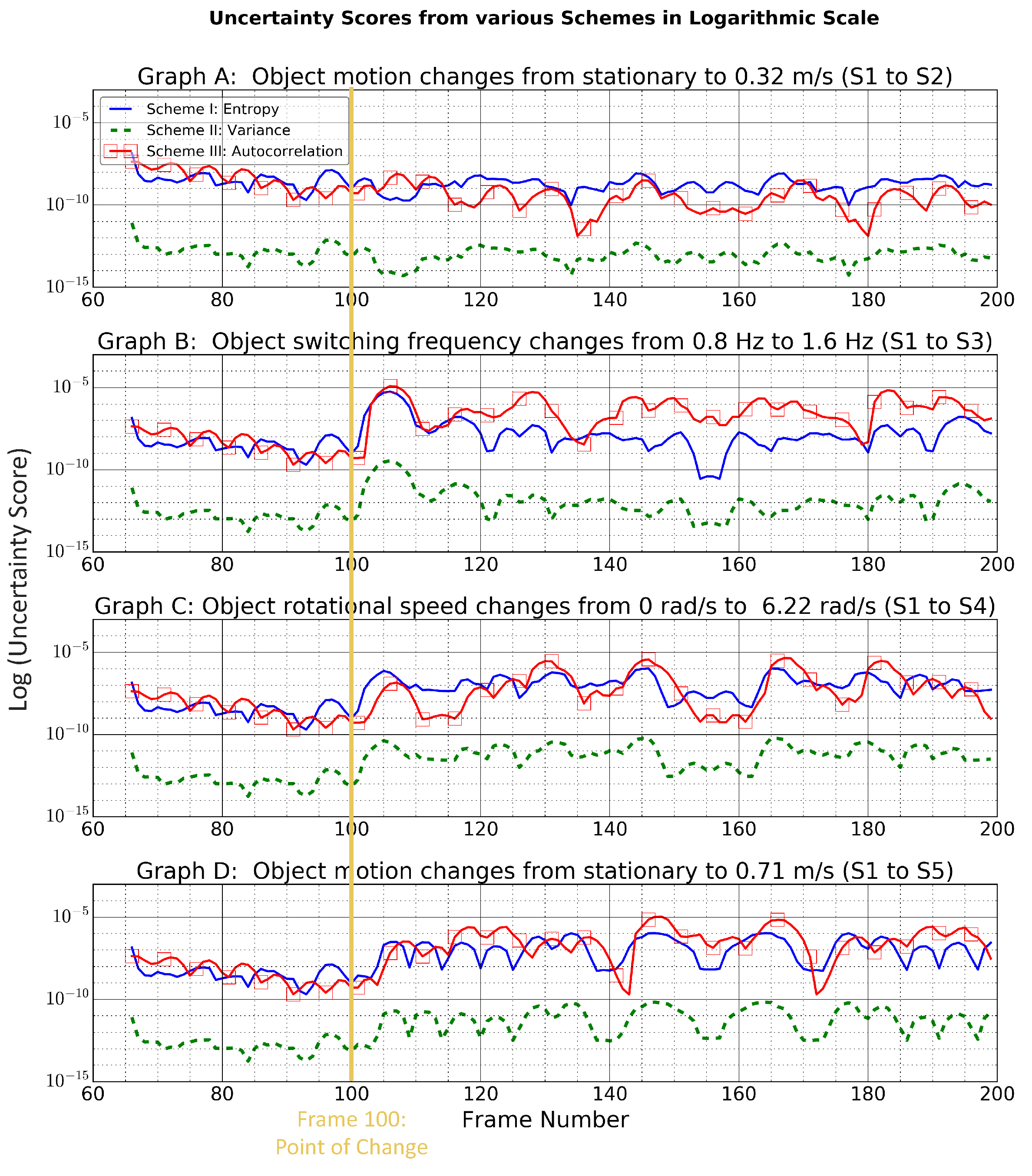
With the interim scores from different schemes, we can then generate the uncertainty scores based on the flow listed in Figure 6 and present the results shown in Figure 7. In the next section, we will evaluate the performances of the three schemes and choose one that best suits our requirements.

8. Uncertainty Estimation Schemes Evaluation

As previously discussed in Section 6, under different scenarios, different window filter settings are preferred. By analyzing the neural network output with the uncertainty estimation schemes, the resultant scores provide an estimate of which scenarios the system is operating under. Then, the window filter settings could be adjusted accordingly. The main objective of the uncertainty estimation schemes experiments was to compare and identify which scheme(s) allow us to distinguish between different scenarios of the operating environment and adjust the window filter settings promptly.

We have experimented with four different events (datasets U1–U4) by combining dataset S1 with S2–4 respectively: object motion changes from stationary to 0.32 m/s (S1 to S2), object switching frequency changes from 0.8 Hz to 1.6 Hz, object rotational speed changes from 0 rad/s to 6.22 rad/s (S1 to S4) and object motion changes from stationary to 0.71 m/s (S1 to S5). To reduce variability in the experiments, the point of change was digitally controlled. Hence, the event mentioned above always took place at frame 100 and was assumed to be an instantaneous change. Figure 7 shows how the uncertainty score from different schemes varies when undergoing changes. Performances of the schemes were evaluated based on processing complexity (i.e., latency), response time and their ability to distinguish among different scenarios.

In terms of processing complexity, entropy is preferred over VAR and autocorrelation. For entropy versus VAR, VAR graphs are simply an offset of the entropy, yet VAR has a slightly higher latency than entropy, as shown in

Table 5. Latency of various uncertainty estimation schemes.

	Entropy	VAR	Autocorrelation
Avg. Processing Time ($\mathsf{\mu }\mathrm{s}$)	93	96	119

; hence, it is less desirable. For entropy versus autocorrelation, they displayed entirely different responses under different settings. The two schemes will be compared in more detail before concluding whether the increase in processing complexity for the autoccorrelation results in a more desirable performance.

In terms of response time, in most cases, entropy shows steeper and faster response compared with autocorrelation, as shown in graphs C,D for point of change (frame number = 100). This shows that entropy is more sensitive to sudden changes, which can be explained because the entropy calculation is based on the current p.m.f. only, while autocorrelation takes into account the temporal dependency among serial data with a lag k; it displays a certain level of memory effect. Hence its changes are more gradual. Steeper changes allow us to be more sensitive to variation in the environment and change to the appropriate window filter configuration more quickly to improve the classification.

In terms of the ability to distinguish among different scenarios, the two schemes are quite similar. For each individual scheme, under different scenarios, the uncertainty scores lies in approximately different ranges.

Therefore, based on our performance metrics, entropy was selected over other methods due to its low latency and quick response.

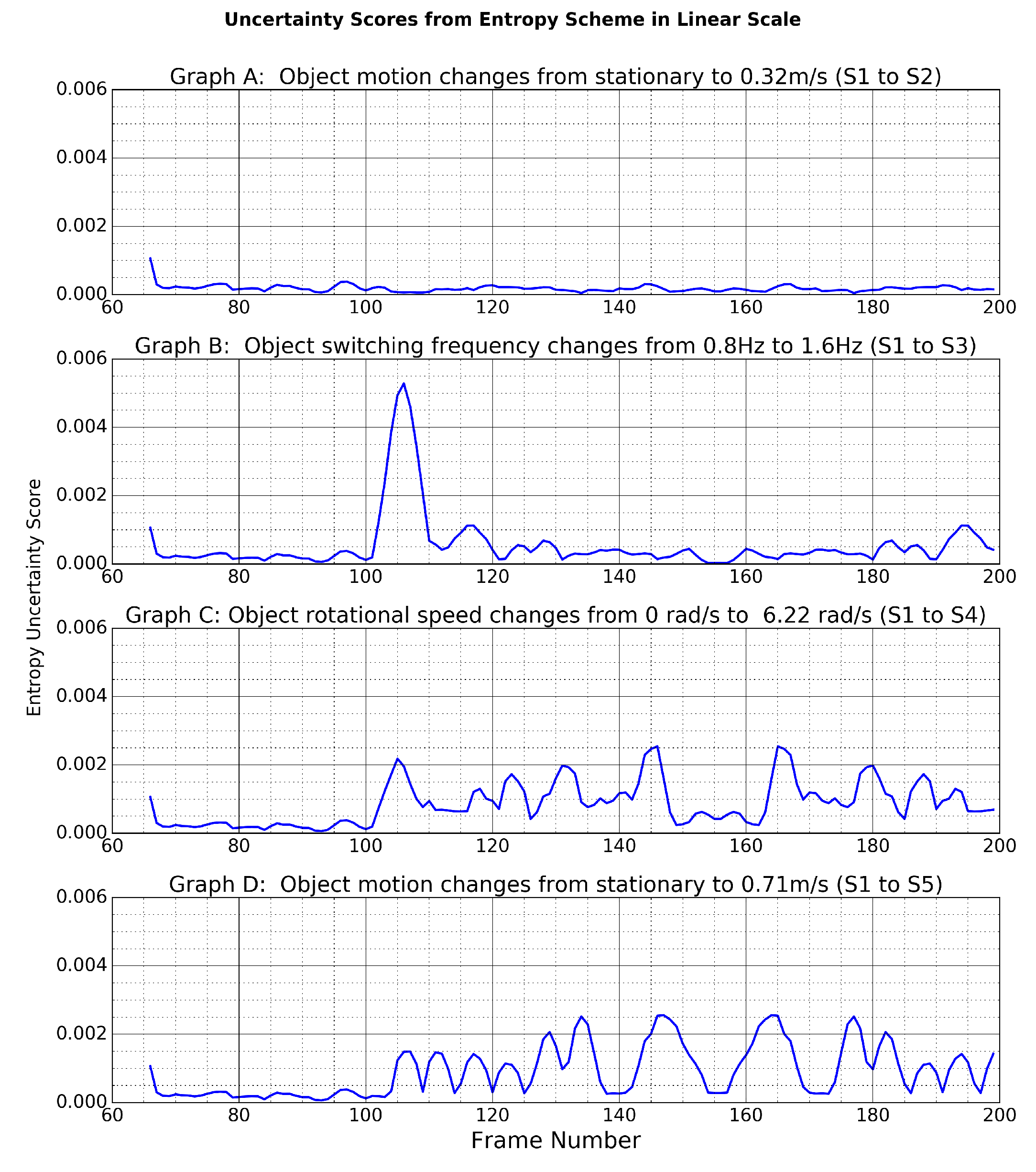
Furthermore, according to Figure 8, we can roughly define the range of entropy uncertainty scores in each scenario:

• In S2 (graph A): scores are below $1\times {10}^{-3}$.
• In S3 (graph B): scores are larger than $4\times {10}^{-3}$ at the point of change.
• In S4 (graph C): scores lay roughly in $1\times {10}^{-3}$ – $2\times {10}^{-3}$ after event happened.
• In S5 (graph D): scores lay roughly in $2\times {10}^{-3}$ – $4\times {10}^{-3}$ after event happened.

These classifications were used to derive a look-up table and the overall adaptive filtering scheme in the next section.

9. Adaptive Filtering

As the last step in formulating our adaptive filter, we would like to derive the lookup table that relates the entropy uncertainty scores with various scenarios, and then map them to the optimal window filter configuration(s) for these scenarios according to Table 4.

Uncertainty scores can help identify the current scenario based on the classified ranges of uncertainty score in Section 8. Meanwhile, optimal window filter configurations can then be chosen for these scenarios based on guidelines in Section 6. As previously mentioned in Section 6, three lists of optimal window filter configurations have been chosen to evaluate the relations between system accuracy and efficiency, as shown in Table 4. Each scheme comprises five window filter configurations; they correspond to the four levels of uncertainty scores and the initialization stage. Combining the information, we can form

Table 6. Entropy uncertainty score look-up table.

Mode	Entropy	Scenarios	Win. Filter Config. (Step Size—Length)
	Uncertainty		Scheme A	Scheme B	Scheme C
0	/	Initialization	1–1	1–1	1–1
1	0–1	Transit to Normal Motion (S2)	10–15	15–15	10–8
2	1–2	Transit to Rotational Motion (S4)	1–10	15–10	15–10
3	2–4	Transit to Fast Motion (S5)	10–13	10–8	10–6
4	> 4	Change to another object quickly (S3)	12–15	15–12	15–12

Scheme A: optimized for accuracy only; scheme B: optimized for accuracy and efficiency; scheme C: optimized for accuracy and efficiency; more aggressive computational savings.

.

Taking Mode 1 as an example: According to Figure 8 graph A (S1 to S2), the entropy uncertainty score is in the range of 0 – 1 $\times {10}^{-3}$. According to Table 3, 10–15 are the window filter settings with the highest accuracy (80%) in scenario 2—region I. Therefore, it was chosen for scheme A. For scheme B, since efficiency was also one of the goals, we wanted to choose settings which decimate frames while having acceptable accuracy, i.e., settings in region II. Therefore, 15–15 with the highest accuracy (78.5%) in scenario 2—region II has been chosen for scheme B. Lastly, for more aggressive computational savings, 10-8, which decimates two frames every cycle and is one of the five settings with the highest accuracy in scenario 2—region II, was chosen for scheme C. Window filter configurations for modes 2, 3 and 4 can be derived similarly. The accuracies and average processing rates of schemes A, B and C were evaluated and compared against the base case in the next section.

10. Overall Accuracy and Performance Analysis

Upon developing various adaptive schemes for the system, we would like to compare their performances against the baseline, a 30 fps basic classification system without any aggregation functions. Figure 9 shows that the baseline system achieved an accuracy of 36.8% while scheme A of our entropy-based adaptive filter achieved 70.6% accuracy with our low precision neural network under diverse environment (self-generated dataset S1–S5). This is a 1.9 times improvement in accuracy. Furthermore, scheme C, the more energy-efficient model, provided an option to reduce average energy by 41.2% compared to scheme A, at a cost of slightly lower accuracy. Our entropy-based adaptive filter features a 29 fps classification rate and a dynamic processing rate up to 142 fps; depending on specific application use case, users can choose to adopt different schemes.

10.1. Energy Consumption of Various Setups

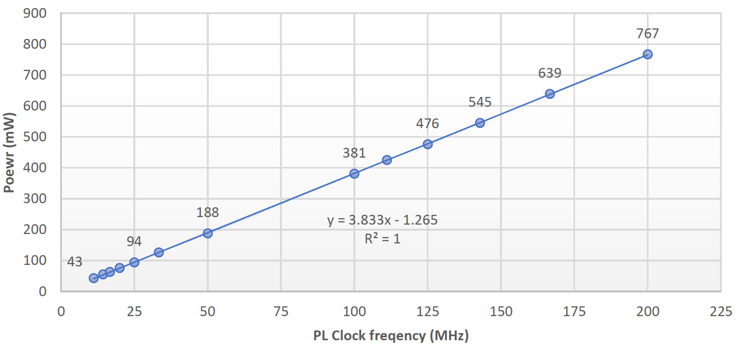
To compare the energy efficiencies of different schemes, we would like to analyze the average energy per second of individual schemes. The inference power consumption at the operating frequency (100 MHz) can be obtained from Figure 10. Then, since the numbers of frames provided to each setup were identical, average energy is positively correlated with processing rate. It can be estimated with the following equation, where latency and processing rate are defined in Equations (1) and (2) respectively:

$$\begin{array}{cc}\hfill \mathrm{Estimated}& \mathrm{Energy}\mathrm{Consumption}\mathrm{of}\mathrm{each}\mathrm{scheme}=\hfill \\ \hfill & \mathrm{Inference}\mathrm{Power}\mathrm{Consumption}\mathrm{at}100\mathrm{MHz}\times \mathrm{Latency}\mathrm{of}1\mathrm{frame}\times \mathrm{Average}\mathrm{Processing}\mathrm{Rate}\hfill \end{array}$$

(12)

The general trend of energy usage can then be inferred from

Table 7. Average energy per second of each scheme (mJ).

	Base	Scheme A	Scheme B	Scheme C
Average Energy per second (mJ)	76	381	264	224

: more complex processing involves higher power usage. Baseline, with a low processing rate and no aggregation functions, has the lowest power consumption. Scheme A, with high processing rate and various filter settings, has the highest power consumption.

For schemes (schemes B and C) that decimate frames and hence, have lower average processing rates, the power consumption is significantly lower than in scheme A while attaining comparable accuracy performance. A dynamic processing rate allows them to use high processing rates (up to 142 fps) when necessary, and decimate frames (lower processing rate) when the operating environment allows it. This resulted in 29.8% and 40.1% lower processing rates compared to the maximum processing rate systems, and hence 30.7% and 41.2% reductions in power. Hence, they are the more energy efficient alternatives to maximum processing rate systems, yet much more accurate than baseline.

10.2. Accuracy Gain under Diverse Setups

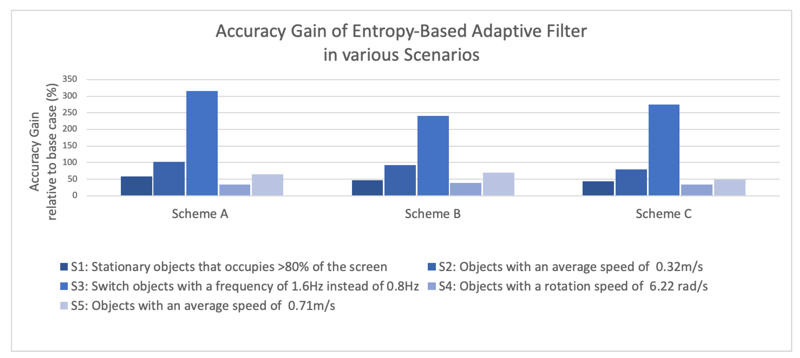
As shown in Figure 11, the entropy-based adaptive filter can provide positive accuracy gain in all scenarios. This can mainly be attributed to the use of high processing rate in combination with the window filter. The information gain helps us to correct classification errors introduced by noise from the image sensor. This proves our hypothesis that by considering more frames, accuracy of low precision neural network can be improved.

It is also worthwhile to note that the accuracy gain was most significant in scenario 3 (switch object in higher frequency) for all schemes; for instance, scheme A tripled the accuracy of the baseline. This can be explained because when we switch the object from one class to another in high frequency, compared to other scenarios, there are more points of change. Hence, there are more opportunities for the system to enter different modes and utilize a more suitable window filter configuration, leading to higher accuracy. This showcases the main advantage of having an adaptive system—it performs much better than the static system in face of high variation in the external environment.

Lastly, it can also be observed that as we progress from scheme A to scheme C, the accuracy gain declines gradually. The progression to a more efficient system comes with a cost in the accuracy. This highlights the trade-off between accuracy and efficiency.

10.3. Overall Performance Gain

With the window filter techniques, we can provide a consistent 29 fps classification rate for users, while varying the internal processing rate. With a much higher internal processing rate, our scheme brings up to 1.9 times improvements to system accuracy. Figure 9 illustrates the correlation between processing rate and accuracy. The base case, with processing and classification rates identical to 29.1 fps, has the lowest accuracy. Meanwhile, the three schemes, which adopted a high processing rate in combination with the window filter, improved the system accuracy from 36.8% to 64.7–70.6%. As aforementioned, this proves our hypothesis that the accuracy of a low precision neural network working with video captured data can be improved by taking into account more frames. In addition, this adaptive system provides us options to save energy while achieving comparable accuracy performance—for instance, schemes B and C reduced energy consumption from 381 to 224 mJ, while still achieving 66.5% and 64.7% accuracies.

Moreover, the trade-offs between accuracy and efficiency can be further explained with schemes A–C. With the uncertainty estimation, we can switch between different window filter configurations dynamically, enabling us to adjust the processing rate based on the current entropy levels of the neural network output. Hence, we have derived schemes A, B and C with different levels of aggressiveness in reducing computation, with A having the most accuracy window filter configurations, yet it does not decimate frames; C has window filter configurations with adequate performance but it decimates more frames. The downward trend in accuracy shows that when more frames are discarded without being processed, the lost information will result in accuracy drops. Thus, there is a trade-off between accuracy and processing effort.

Lastly, our entropy-based adaptive filter allows the underlying processing to occur at a higher rate (142 fps), while the on-screen classification labels are updated at an arbitrarily slower rate, e.g., 29 fps, as explained with Equations (2) and (3). The output will flicker less compared to the high processing rate-high classification rate system, yet with much more accuracy than low processing rate-low classification rate system. This provides a much more pleasant user experience.

11. Conclusions

This paper has demonstrated how by considering more frames, the accuracy of a binary precision neural network can be improved in a real application scenario with data captured via a camera. We have created a novel pipeline that dynamically adjusts processing rate based on the entropy present in the neural network output. Our entropy-based adaptive filter successfully enhances the system accuracy from 36.8% to 70.6% relative to the baseline. The 1.9 times accuracy improvements can be attributed mainly to the 4.9 times higher processing rate. The adaptiveness introduced to the system enables the automatic variation of the processing rate based on the complexity of data, which could be very useful to improve overall energy efficiency. Furthermore, this approach does not require changes to the hardware-accelerated neural network so it could be applied to other hardware accelerators. It can be considered orthogonal to research in hardware acceleration instead of a direct comparison, since it proposes a general mechanism to adjust the operating point of a neural network system to better track the input data complexity and to obtain better accuracy with a constant classification rate using a variable processing rate. For instance, a high processing rate is used for more complicated inputs and vice versa. Furthermore, our design is not dedicated to improving the workings with standard datasets that contain single frames and consequently cannot be combined in image groups with different features; rather, it focuses on working with real video streams affected by image sensors’ artifacts, etc. Therefore, our approach aims to enhance the state-of-the-art classification methods rather than compete with them.

Future work involves:

• Energy Savings: Our adaptive processing strategy coupled with the energy proportional binarized network presented in [6] to measure the obtained energy savings while processing real video streams.
• Scale up for larger scale networks: Our FINN accelerator is limited to a low resolution (32 × 32) input due to constraints on the memory capability of the Zynq Z7020 device used in this research. Future work will consider larger scale networks for more complex datasets like Imagenet.
• Adopt more powerful hardware: Our current approach utilized both PS and PL, because in Zynq Z7020, the PL BRAMs are already fully occupied by the neural network hardware. In the future, it would be useful to explore implementing the system on more powerful FPGAs, such as Ultrascale MPSOC. This will enable our design to run on PL exclusively, which generates better performance and increases the maximum processing rate.
• Performance on a fixed processing resources system: With scheme B, we explored the idea of dynamically decimating frames, while achieving a high accuracy. It would be interesting to compare it against a fixed processing resources system with the same goal. Hence in the future, we can explore more on the performance of fixed processing resources systems, which would then allow us to draw a more comprehensive comparison between the static and dynamic systems.

To encourage further work in the field, the system is available open-source at https://github.com/elimkwan/Entropy-Driven-Adaptive-Filter-for-FPGA-Object-Recognition-System.