1. Introduction
With the growing scarcity of fossil energy, the use of sustainable energy for power generation has increasingly attracted the attention of global power industry. The fact that solar energy is the largest sustainable energy source has put photo-voltaic (PV) power generation in the spotlight. However, because the output power depends on variable meteorological factors, the PV generation system reveals a high level of uncertainty and periodicity. The integration of large scales PV energy into the power grid will challenge the power balance of the grid, leading to a series of disturbance. Therefore, the development of large-scale grid-connected PV power plants is limited [
1]. The accurate prediction of PV power generation is an effective way to provide guidance for grid operation scheduling and regulation of the PV system itself, and to reduce the instability of PV grid-connected operation. These are strong motivations for ultra-short-term forecasting of the output of PV power plants.
In terms of the specific forecasting horizon, the forecasting can be divided into: ultra-short-term forecasting (a few minutes to 1 h ahead), short-term forecasting (1 h to several hours ahead), medium-term forecasting (several hours to one week ahead), and long-term forecasting (one week to one year or more) [
2]. According to different forecasting logics, PV power generation forecasting methods are often classified into two basic types: direct forecasting methods and indirect forecasting methods.
The direct forecasting methods are linear modeling methods, which are also known as classical physical modeling methods. These methods combine the geographical location and numerical weather forecast of the PV generator in order to obtain solar vertical illuminance data, and then the principle of physical power generation of the PV system is used to develop linear mathematical models of PV power generation; finally, the output power of PV systems is directly predicted, without historical power generation data [
3,
4,
5,
6].
The indirect forecasting methods are non-linear forecasting methods, which mainly contain statistical methods [
7] and machine learning methods, such as nonlinear multivariable regression [
8], support vector machine [
9],
k-means clustering [
10], artificial neural network [
11,
12], etc. The physical principle of PV power generation is not considered in these methods, while historical output power data and meteorological environmental factors are analyzed generally. Subsequently, these methods can obtain the output power of the system based on the PV power generation forecasting model.
From the articles published in recent years, the machine learning methods were increasingly applied to build PV power forecasting models by relevant scholars [
13,
14]. For example, a prediction model inspired of similar-day detection engine was proposed for day-ahead small-scale solar power output forecasting in [
15]. In [
16], a high-precision deep neural network model was proposed, in which the PV output in the next 24 hours was predicted. The results verified that the PVPNet algorithm for short-term forecasting achieved good forecasting performance combined with strong generalization ability; however, the quantity of input features was relatively too large. In [
17], a grey-box model that is based on the hourly forecast of the global irradiance and quantile random forest model consisting of multiple classification models were discussed. The results showed that the improvement of more complicated approach was consistent over months in a year. In [
18], a PV model was constructed upon the quantile regression forests, which was trained with forecasts of several meteorological variables that were produced by a numerical weather prediction model, and spatial and temporal indexes was estimated from the forecasted variables. A median and confidence interval were calculated in order to predict the hourly power of the PV plant. In [
19], a statistical spatio-temporal method was proposed to forecast PV plant power output in six hours. A procedure inspired from the clear sky index for solar radiation was employed to address the non-stationarity issue of the production series. In [
20], the aerosol index, which was able to detect the presence of UV-absorbing aerosols such as dust and soot, was added to the input data of a one-day-ahead PV output forecasting model based on BP neural network. When compared with a model that only choses traditional input features, the precision of the model using the aerosol index was indicated to be highly improved in both sunny and cloudy weather conditions.
In addition, the combination of artificial neural networks and various other methods were applied to the study of PV output forecasting [
21,
22,
23,
24,
25,
26]. For example, the statistical features of historical PV power time series were extracted by the stationary wavelet transform (SWT) that was proposed in [
27], and a final deep neural network (DNN) was designed to make use of the reconstructed values estimated by four LSTM networks to predict the final forecasted value of the next 30-min. PV power. The grey theory was used in data processing in order to improve the forecasting accuracy and address the over-fitting problem presented in [
28]. A deep belief network (DBN) model was combined with a feed-forward network (FFN) for day-ahead PV power output forecasting, which was superior than DBN alone in forecasting accuracy. Bayesian optimization in [
29] was applied to select the optimal combined features, and a deep learning model was constructed based on a LSTM block and an embedding block with the connection of a merge layer in order to predict the day-ahead PV power output. A support vector regression (SVR) method was proposed in one-hour-ahead PV power prediction [
30]. Big data and minimum redundancy maximum relevance (mRMR) technology were applied to input features dimension reduction, while GA was used to optimize the learning parameters inside SVR machine; thus, the computational speed and the forecasting precision were both increased. The wavelet packet decomposition (WPD) in [
31] was utilized to decompose the original PV power series into four sub-series, each of which was fed into a LSTM networks. Subsequently, the final one-hour-ahead PV power forecasting results were obtained via a linear weighting method, reaching an average RMSE in four seasons of 0.2357 kW. In [
32], a Weight-Varying Combination Forecast Mode (WVCFM) model was developed in order to generate deterministic point predictions for following 5 min, achieving an mean absolute percentage error (MAPE) under
. In [
33], the radiation classification coordinate (RCC) method was applied to process data set, and the RCC-LSTM model reached MAPE of 2.74∼7.25% in predicting the PV power generation of a next day. A novel hybrid improved Kmeans-GRA-Elman (HKGE) model was proposed in [
34] for one-day-ahead PV power prediction with one-hour interval. The average daily root mean square error (RMSE) and R
of the HKGE model are 4.3210 kW and 0.9953, which outweighed other eight compared models.
However, these existing indirect forecasting methods are generally employed in a large forecasting time span, ranging from several hours to one day, and the model structure or the data processing method was complex, while the forecasting accuracy is limited. Meanwhile, the problem of how to accurately predict the PV power in ultra-short-term, reduce the complexity of the network structure, and improve the calculation speed and forecasting accuracy, has not been well solved.
In this paper, the ultra-short-term forecasting method that is based on radial basis function (RBF) neural network for solar PV power generation is investigated. RBF neural network is characterized by simple structure, good generalization ability and fast learning convergence rate. To promote these advantages, the superior limit number of hidden layer neurons is set. Moreover, the input of neural network is reduced according to their Spearman correlation with the power value to be predicted. To reduce the calculation errors, the data are normalized. To improve the forecasting accuracy in generating next 15 min, forecasts, the expansion parameter of RBF neurons is adjusted continuously, which affects the sensitivity of neurons to the input data. From the comparison with other three existed forecasting model, it is verified that the proposed model achieves excellent performance in both forecasting accuracy and robustness.
The paper is organized, as follows. In
Section 2, the mathematical principle and hyperparameters of RBF neural network are presented. In
Section 3, the obtained sample data are prepossessed. In
Section 4, the forecasting model is proposed, appropriate parameters are determined via repeatedly tests, and the experimental results and comparisons with three existed forecasting methods are analyzed. Finally,
Section 5 gives the conclusions.
2. Mathematical Model of RBF Neural Network
2.1. Structure of RBF Neural Network
The RBF neural network is a forward neural network. It is a three-layer feed-forward neural network that is based on high-dimensional spatial interpolation technology. RBF is designed as the activation function of the neuron, making the RBF neural network able to approximate any continuous function with arbitrary precision. Thanks to the strong nonlinear approximation combined with the simple network structure, it is often used for function approximation and analysis.
When compared with the more well-known standard back-feed propagation neural network (BPNN) that requires multiple hidden layers, the RBF neural network only employs one hidden layer. To achieve the same training accuracy, as a local approximation network, the later often spends less training time than the BPNN. Moreover, when the number of training samples increase, the performance of RBF network learning is better [
35]. Therefore, in this paper, the RBF neural network is used to approximate the ultra-short-term output of the PV power generation system.
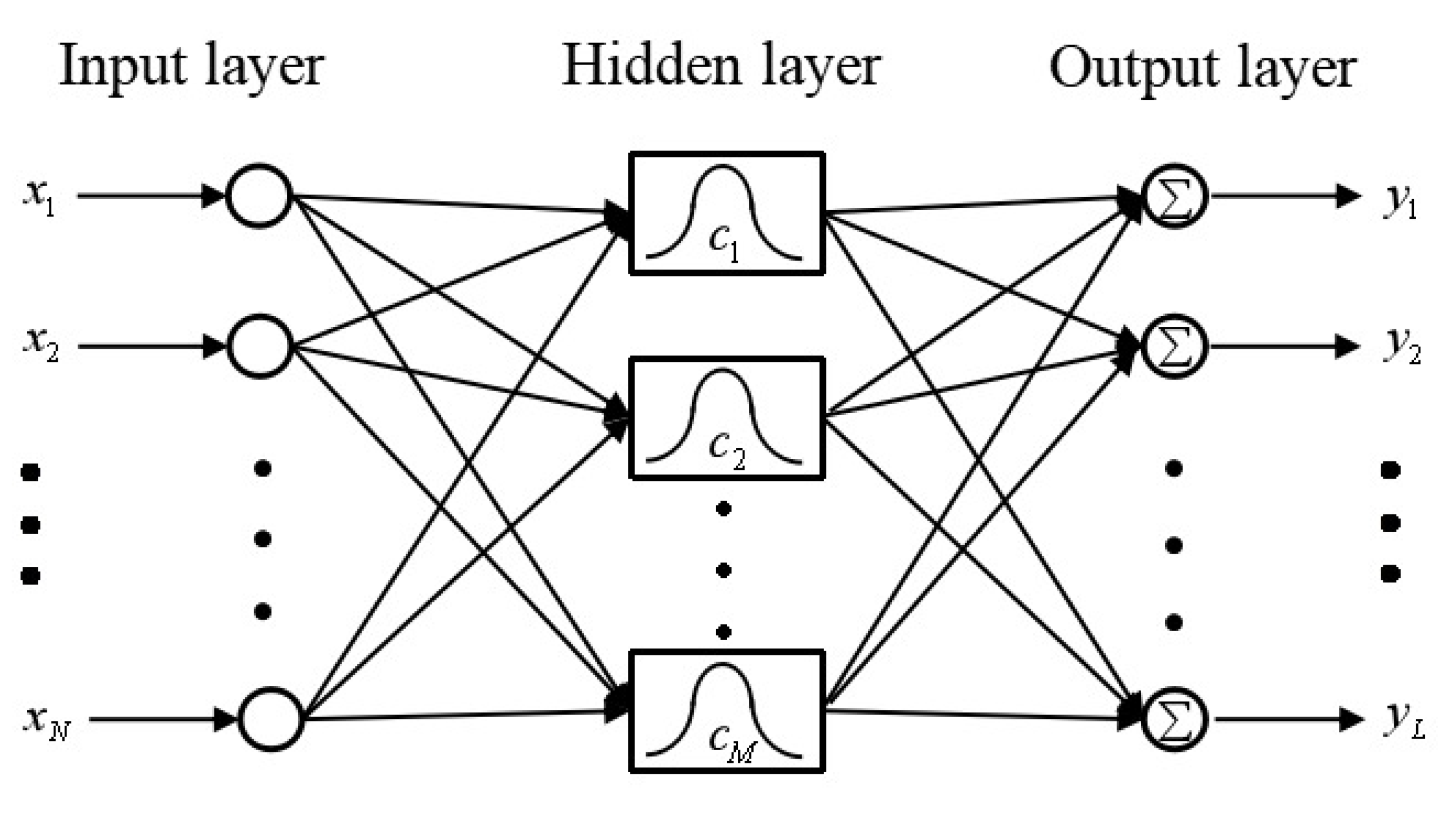
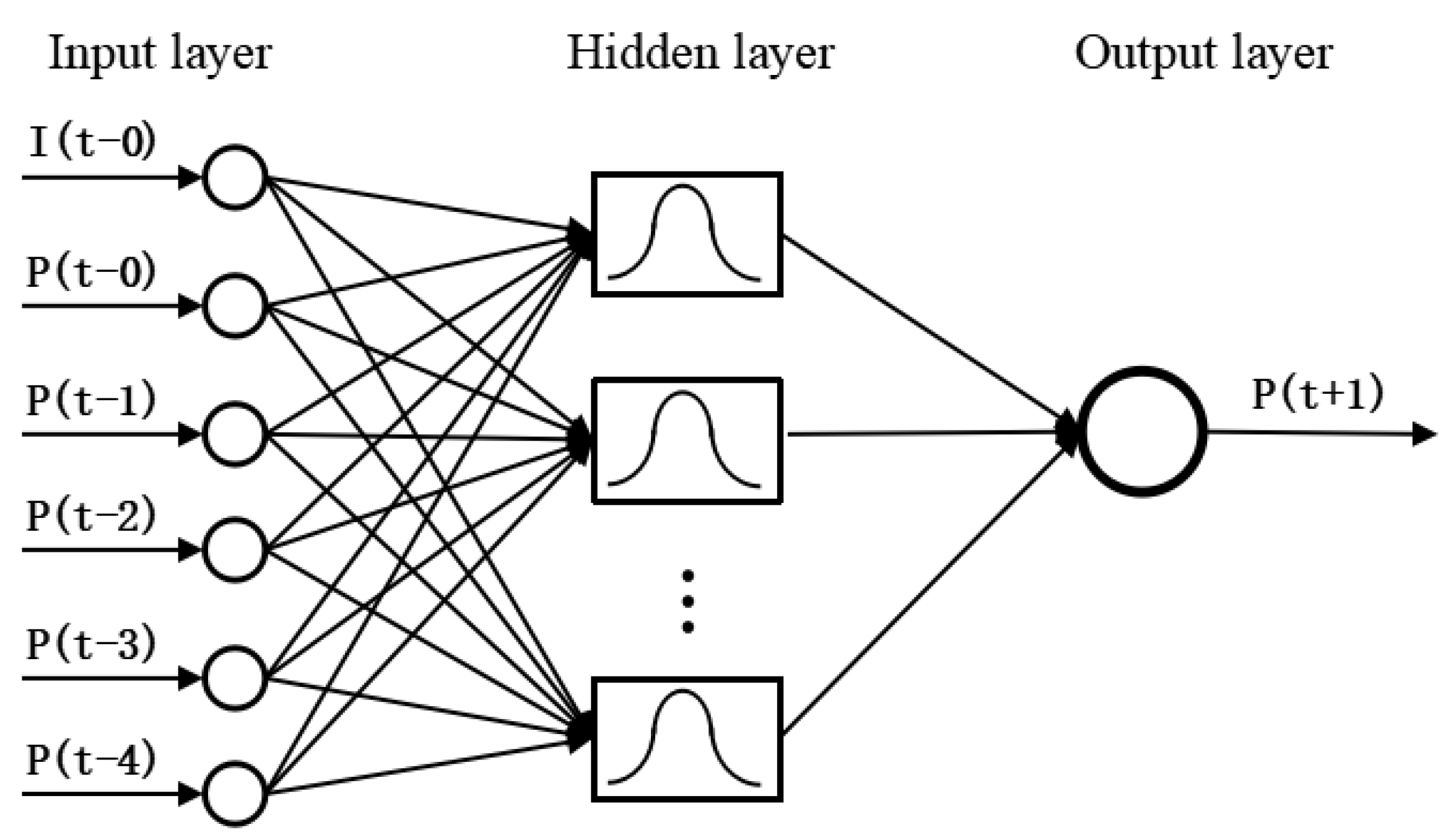
The standard form of the RBF neural network is a fixed three-layer structure of “input layer-hidden layer-output layer”. The structure of the RBF neural network in the form of “
N-
M-
L” is shown in
Figure 1 [
36].
Here, denotes the data fed into i-th input node, N denotes the number of input nodes. denotes the center vector of the j-th radial basis neuron and M denotes the number of radial basis neurons in the hidden layer. denotes the k-th output and L denotes the number of output nodes.
The first layer of RBF neural network is the input layer. The number of nodes in this layer is the same as the dimension of input vectors. The input layer only plays the role of transmitting signals, so that the input vectors can be directly fed into the hidden space.
The second layer is the hidden layer, which is the most critical layer of the RBF neural network. The activation function that is used in hidden neurons is the RBF, as the previous section introduced. The number of RBF neurons in this layer depends on the complexity of the problem to be solved and the amount of data provided. In fact, RBF neurons only respond to a relatively small area of the input space, resulting that the larger number of input vectors and its ranging, the more RBF neurons required in order to achieve the same training accuracy. The goal of this layer is to perform a non-linear transformation of the input vector from the input space to the high-dimensional feature space (usually
). Subsequently, in this high-dimensional feature space, a linear model is employed in order to train samples. Thus, through spatial transformation, a non-linear problem is transformed into a linear problem, thereby simplifying calculations. The process of training the hidden layer can be described as adjusting the parameters of the activation function, including the center vectors and the thresholds. A nonlinear optimization strategy is applied in this process, so the learning speed is comparatively slower than other layers. The output
of
j-th neuron in hidden layer can be calculated as
where the input vector
denotes the position or coordinate of the input and
denotes
N-dimensional real number space.
denotes the center vector or the position of
j-th neuron in hidden layer, also called the weight vector of the neuron.
denotes the dot product of the input vector
x and the center vector
, which is also known as the Euclidean distance, and it is calculated, as follows:
denotes the threshold or sensitivity of j-th node in hidden layer with the superscript presenting the hidden layer, and this parameter regulates the response range of neurons to the input intuitively.
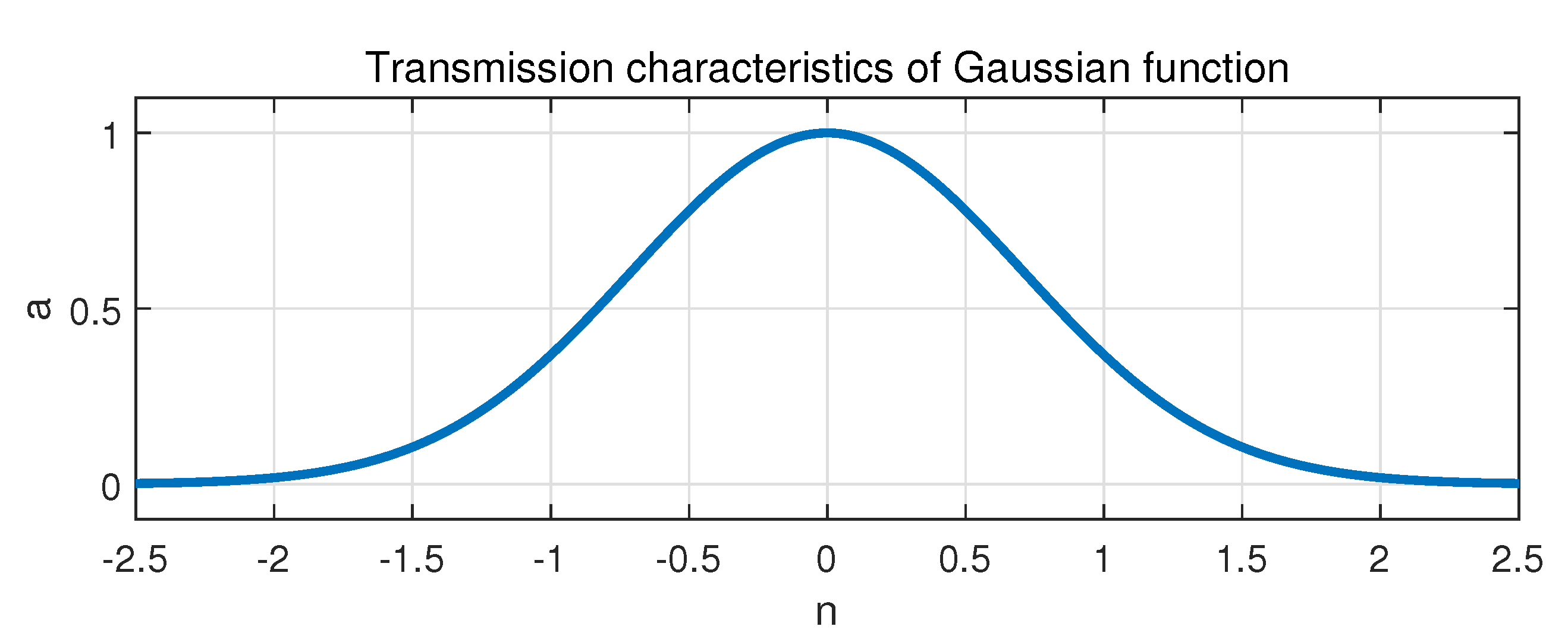
denotes the radial basis activation function of the RBF neuron, which is a radially symmetric and non-negative function. The Gaussian function is often chosen as the radial basis transfer function in RBF neural networks because of the excellent properties of smoothness, radial symmetry, and simple form. The Gaussian function is demonstrated in
Figure 2, with
n denoting the input of the function and
a denoting the output, and the relation between them is expressed as
The third layer is the output layer, and the number of nodes in this layer depends on the dimension of the output vectors. The output of each hidden layer neurons is linearly weighted, and then the final output of RBF network is generated in this layer. The linear optimization strategy of the LS method is applied in training the linear weights in output layer, leading the learning speed relatively fast. The output
of
k-th node in the output layer can be expressed as
where
denotes the weight of
j-th RBF neuron to
k-th output node, and
denotes the threshold of
k-th node in output layer with the superscript presenting the output layer [
37].
2.2. Learning Algorithm of RBF Neural Network
The precise and approximate RBF neural network design functions are provided in the MATLAB platform. The precise type makes the number of hidden layer neurons directly equal to the number of training input samples, and its calculation speed is consequently fast, while the approximate type sets the upper limit of the number of hidden layer neurons, which is more effective when the number of training samples is large [
38]. Obviously, the approximate type is more suitable for the case of more than 10,000 sets of data in the training set of this paper.
The function in MATLAB to design an approximate radial basis network is , where the parameters P, T, , , M, and denote the input matrix, output matrix of the training set, the mean squared error goal, the maximum number of hidden neurons, and the number of neurons to add between displays, respectively.
With the target error and maximum number of hidden layer nodes set as an M separately, the training process of the approximate RBF neural network with training set data is as following.
Step 1: calculate the loss function of the simulating network with all the training samples. According to the LS method, the loss function can be expressed as
where
N denotes the number of training samples in training set,
denotes the forecasting output of the model, and
denotes the true output.
Step 2: find the sample x that contributes the most to the network error.
Step 3: add a radial basis neuron to the hidden layer, and set its center vector
c to the transpose of the input vector of the training sample, which is
and set its threshold as
b, which is determined by another parameter
in MATLAB as following.
which means that the neuron responds an output higher than
to any input vector with an Euclidean distance to its center vector within the value of
.
Step 4: readjust the weights of each neuron in the hidden layer to each neuron in the linear output layer according to LS method, in order to minimize the network error after adding RBF neurons.
Step 5: re-update the MES of the network. Repeat the previous steps 2 to 4 until the specified error performance index is met, or the upper limit of the number of hidden layer neurons M is breached.
As the steps finished, the function returns a new radial basis network .
3. Data Analysis and Process
The data
https://www.dcjingsai.com/v2/cmptDetail.html?id=309 used in this article are the meteorological data and power generation data of one PV power station in China from 1 January 2017 to 15 November 2018
https://github.com/AceBBang/PV-forecasting-data. Meteorological data and power generation data are measured at 15-min. intervals. In order to simplify the experiment, the data at night and invalid data are excluded. The invalid data mainly include some days with no change in solar irradiance, PV power output, or other types of data. Finally, more than 20,000 sets of data are obtained, including wind speed, wind direction, ambient temperature, pressure, humidity, solar irradiance, and power generation at 48 quarters during the day time.
3.1. Data Analysis
Solar panels for PV power generation rely on radiant energy in sunlight and the “PV effect” of the panels to generate electricity. Their working conditions are subject to two major factors. One is the internal electrical properties of the PV power plant, including the efficiency of photoelectric conversion devices, aging degree of PV modules, ash accumulation of PV array panels, differences in installation of panels, performance differences of transmission lines and inverters, losses in power conversion and transmission, etc. The other type is relatively external environmental factors, not only meteorological environmental factors, such as solar irradiance, weather type, season, temperature, wind speed, and cloud cover, but also geographical environment factors, including latitude and longitude of the PV system, topographical conditions, and nearby buildings.
For a given PV power plant, all output power data are provided by the same set of PV power generation components. Therefore, the time series of historical power generation has taken the impact of system information and internal factors of the PV array into account. Moreover, during the service life of the system, most of the qualified PV inverter modules operate in a relatively stable state for a long time. Although the power conversion efficiency and photoelectric conversion efficiency can change with time, the amount of change over a long period is so slight that it can be considered to be constant in short-term forecasts. Therefore, it is not necessary to consider the factors that are implicit in the historical output power data, including the power conversion efficiency of the inverter, the PV conversion efficiency of the PV array, the total area of the PV array, and the geographical environment of the power station.
Distinct from the geographic environmental factors and internal electrical factors of PV power plants, meteorological environmental factors, such as solar irradiance, ambient temperature, and humidity, can experience active changes. Even within a few minutes, non-negligible fluctuations can occur, and it is verified that they introduce a large influence into the performance of power generation [
39,
40]. Accordingly, meteorological factors should be taken as input features of the forecasting model.
Because of the hysteresis of photoelectric effect, there is inertia behind changes in its influencing factors, such as solar irradiance and ambient temperature. The time series of PV power station power generation shows a high autocorrelation, which is known as the sequence correlation. This means that the output power value at the next time step is closely connected with the outputs of the several historical time steps. Therefore, in addition to the meteorological environment factors, another important input feature is the historical power generation data of the PV system.
However, the amount of meteorological data and historical data are too large and, if a large amount of input features are fed into the network, the speed and accuracy of network calculation would be greatly reduced, and the computational burden of the network would be increased. Therefore, it is necessary to select some features with high correlation with the output power of the time to be predicted. Moreover, the correlation coefficients between these feathers and the data to be predicted are required.
In statistics, the Pearson correlation coefficient is commonly used to measure the degree of correlation between two sets of data, but it requires that the data of the two variables are normally distributed as a whole, and only the linear correlation and direction of the two variables are given. When compared with this, the analysis of Spearman correlation coefficient pays more attention to whether the changing trends of the two variables are the same, and it is less sensitive to anomalous data and more applicable. Thus, the Spearman correlation coefficient is more suitable for the non-linearity of PV power generation forecasting studied in this paper. The Spearman correlation coefficient between set
and set
can be expressed as following,
where
and
is the rank of elements
in
and
in
, respectively.
and
is the average of the rank of all elements in
and
, respectively.
N is the number of elements contained in
and
. The ranking method can be described as: every element is arranged in descending order, with the corresponding rank of the largest value being 1 and the smallest
N. If there are equal values of some elements, then the rank of these elements takes the average of the positions of these equal elements.
The function in MATLAB calculates the Spearman correlation coefficient between and , returning the number .
To choose the highly correlated features,
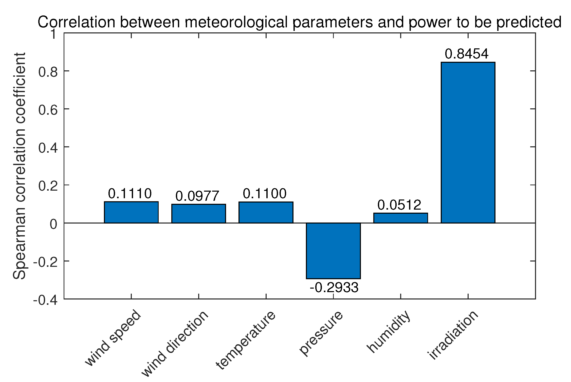
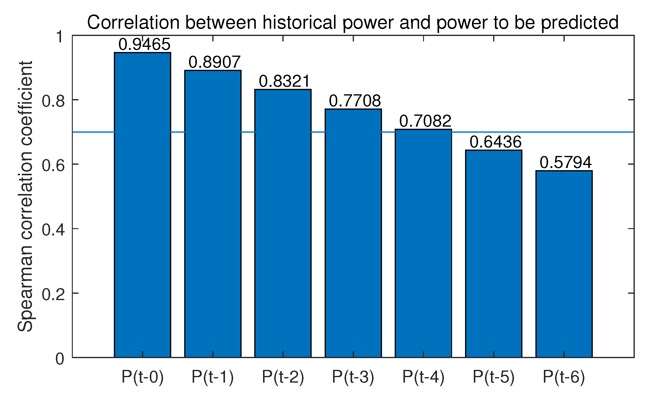
Figure 3 and
Figure 4 shows the correlation coefficient between the power value 15 min later, the moment to be predicted, and meteorological data and historical output power data, respectively, with the specific results of the correlation analysis on these variables labeled. The label
presents the output power before
i quarter or quarters.
It can be seen from
Figure 3 that only the correlation of irradiance reaches above
, while the correlation coefficients of other meteorological parameters are all below 0.5. Meanwhile,
Figure 4 illustrates that the correlation generally decreases with the increase of time interval. Therefore, in order to ensure the input features quality and streamline the features, irradiation
, generated power
,
,
,
, and
with
are selected as the input features for the forecasting model.
3.2. Data Processing
When considering that RBF neural network learning belongs to supervised learning, this paper divides the sample data into three data sets according to a certain ratio: a collection of data constitutes the training set, which is used to train the forecasting model under different hyperparameters, including the number of hidden layer neurons, sensitivity coefficient, target error, etc. is divided into the validation set, which is used in orderto verify the forecasting accuracy of the trained neural network, so as to select the most suitable hyperparameters. Finally, the rest is the testing set, which is used to finally check the generalization performance of the forecasting model.
The solar irradiance and PV power generation been chosen as features with different orders of magnitude and dimensions, using data directly may lead to low network convergence speed, oversaturation of hidden layer neurons, numerical problems (i.e., due to the calculation accuracy of MATLAB, in the case of a large difference in the order of magnitude, the two quantities that are actually obviously equal will be misjudged as unequal), and other problems. Therefore, before the network training, the data should be normalized. When considering that the average relative error percentage is needed later, in order to avoid the result that the relative error is calculated as infinite when the original output is 0, all the data in the training set are normalized to the interval .
The formula for normalizing set
to set
is as following
where
x is the element to be normalized in the original sequence and
y is the corresponding element after normalization,
and
are normalized interval boundary values, which are
and
here,
and
are the minimum and maximum values in the to-be-processed set
, respectively.
The function provided in MATLAB returns the normalized set and the process settings, which are and .
Subsequently, with the function
, testing set data combined with validation set data can be normalized according to (
9) applying the same
and
as in training set.
All of the forecasted value will be reverse normalized before the final forecasted results are obtained through the function .
3.3. Performance Metrics
The PV power forecasting model is used in order to predict the amount of power generation, and the pursuit of constant research, modeling, and improvement is to continuously reduce errors. Therefore, scientific evaluation of errors is particularly important. There are five common types of performance evaluation index tables for the power forecasting model used in [
41].
The mean bias error (MBE)
where the
N is the number of testing instances,
is the forecasting output of the model, and
is the true output.
The mean absolute error (MAE)
The mean absolute percentage error (MAPE)
The mean square error (MSE)
The root mean square error (RMSE)
4. Experiments and Results Analysis
This section reports the process of model establishment and the experiment and comparison results for performance evaluation in order to validate the effectiveness of the proposed model.
4.1. Model Establishment
The six-dimensional data with high correlation with power
are selected as the network input features to predict the PV output. The input features consist of the solar irradiance at current moment
and the PV output at current as well as historical moment, including the PV output from
to
, while the network output is
, the output of the PV power generation system at the next moment.
Figure 5 shows the "6-input-1-output" RBF neural network structure to be used in this paper.
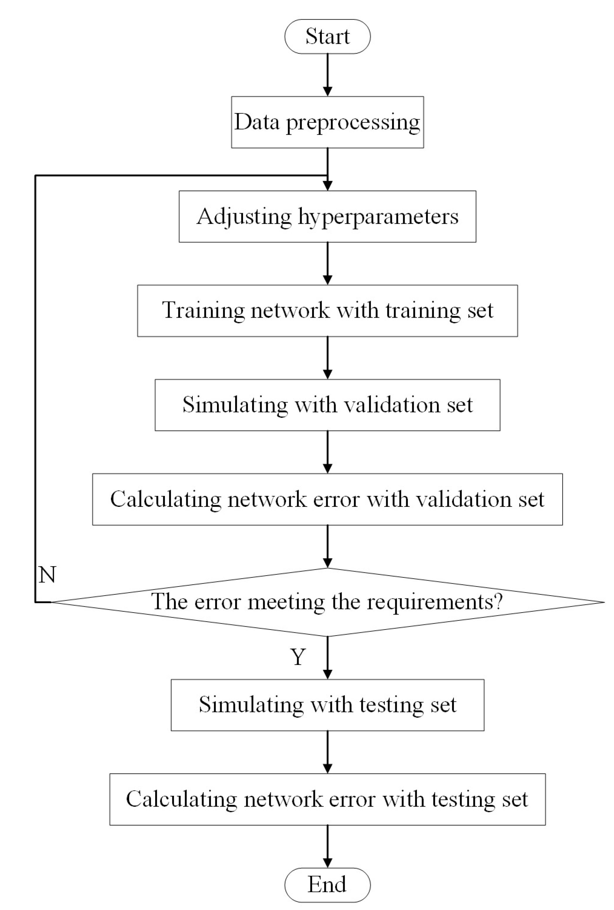
After the training data, validation data and the test data divided in the previous section, the proposed PV power forecasting model is established according to the process that is shown in
Figure 6.
The PV power forecasting model is generated with the training function of approximate RBF neural networks on MATLAB, which means fewer hidden layer neurons than the number of input data sets are required for training.
Subsequently, the training set and the verification set are simulated respectively through the simulating function to optimize the model parameters. In this process, the iterative trial method [
42] is applied in order to optimize the maximum of hidden layer neurons and the expansion parameter
. With the optimized model, the samples of testing set, which are not applied in the adjusting process, are used to test the performance of the forecasting model.
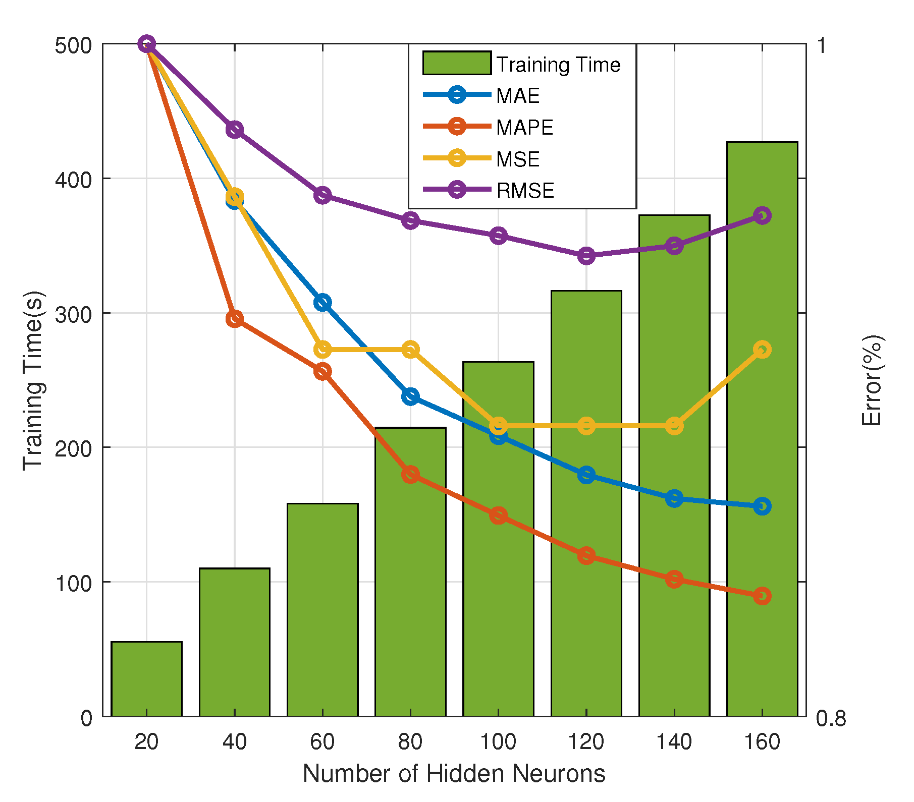
After several experiments, it is found that the greater the number of hidden layer neurons, the higher the learning accuracy, but the slower the training speed,, as illustrated in
Figure 7. For clear demonstration, the error denotes the ratio of each error type with different hidden neurons to the corresponding error of the model with 20 hidden neurons with a fixed
on validation set in
Figure 7. When there are 120 neurons in the hidden layer, a better learning performance can be achieved, and the calculation speed of the training is not too slow with the training time slightly higher than 300 s. In addition, as the hidden neurons increased, the MSE and RMSE begin to increase again.
The expansion parameter in MATLAB functionally replaces b, and it adjusts the sensitivity of the hidden layer neurons to the input vector. The value should be large enough for the RBF neurons to respond to overlapping areas of the input space, but a too large may lead to all neurons responding to various input in the same degree. Hence, it is necessary to call the RBF network design function multiple times with different values and try to find the best value. Based on this, the RBF network design function is called in a loop structure with Continuously changing s. When comparing the errors in different cases, the expansion parameter with effective performance is selected. The learning effect can be demonstrated by small error in the training set, and the generalization ability can be proved by small error in the testing set.
The predetermined requirements that are mentioned in the flowchart mainly include that the RMSE of both the training set and the validation set drop below 10%, and the gap is not too large. Finally, under the premise of ensuring that the learning effect and generalization ability meet the requirements, the expansion parameter is set to be . Additionally, the structure of RBF neural network is “6-120-1” structure, which means 6 nodes in the input layer, 120 neurons in the hidden layer, and 1 output node.
4.2. Results Analysis
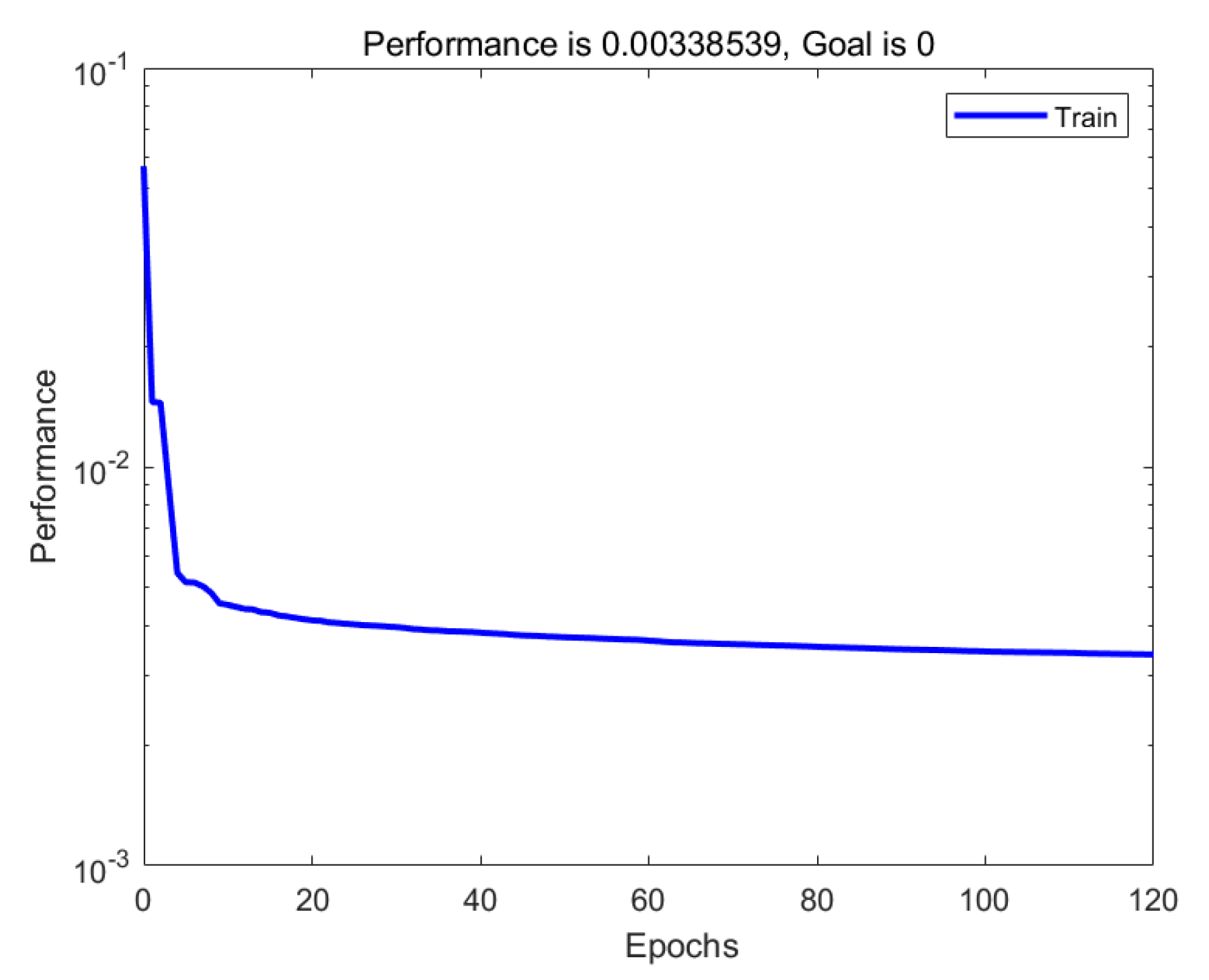
Figure 8 shows the mean square error (MSE) curve of the training set in the process of gradually adding hidden layer neurons to the forecasting model.
In
Figure 8, the horizontal axis denotes the number of epochs, and in each epoch the entire training set data is passed forward the neural network once. One hidden layer neuron is addicted after each epoch during the RBF neural network training process. The vertical axis is a logarithmic axis, denoting the MSE value of the network, which highlights the magnitude of the error. The curve shows that, with the continuous increase of radial basis neurons, the magnitude of the network error decreases rapidly at first and then gently, which illustrates the convergence of the algorithm clearly.
Next, the training set, validation set, and testing set are separately simulated, and various errors of the three data sets are calculated.
Table 1 shows the specific values of the five types of error evaluation indicators for these three data sets.
MBE is the average of the bias errors of the output by the network, which is also known as the average error, and it reflects the overall average deviation of the predicted value from the true value. The MBE of the verification set is greater than 0, and the test set is less than 0, which indicates that the predicted value of the PV power ultra-short-term forecasting model is generally higher for the validation set and lower for the testing set, respectively.
MAE is the average value of the absolute error of the predicted output. Analyzing it can avoid the situation where the positive and negative errors cancel out; thereby, the total absolute error reduced to a certain extent. Therefore, MAE can better reflect the magnitude of the absolute error between the predicted value and the actual value than MBE. The MAE of all three data sets is greater than the absolute value of MBE, which means that the error values of the forecasting results of the model are offset partly.
MAPE refers to the average value of the absolute value of the relative error between the predicted value and the true value, and then multiplied by . This indicator can well reflect the degree of confidence in the forecasting. The MAPEs of the training set, validation set, and testing set all drop less than , meeting the main requirements for the forecasting model in the previous section.
MSE is the default evaluation index for measuring network errors when MATLAB creates a neural network primarily owing to its simple calculation, presenting the sum of the absolute errors. The MSE of each data set is between and , which means that the learning effect of the forecasting model is better.
The RMSE is calculated from the square root of the mean square error. Its value is particularly sensitive to the maximum and minimum errors in a set of predicted values, so the dispersion of the forecasting can be well indicated. The RMSEs are all around , indicating that the deviation between the predicted value and the true value is very slight, and the forecasting model reaches a high degree of confidence.
The generalization performance of the model refers to robustness, which is, for untrained data, the forecasting model can also give forecasting values close to the true value. Therefore, a large testing set error is equivalent to the poor robustness of the model. From the simulation results, the low error of the testing set (the MAPE is below and the RMSE is slightly above ) fully reflects the high generalization ability of the model, and it is indicated that the forecasting task for the unlearned samples is finished accurately.
From the training set, the number of neurons in the hidden layer of the model is 120, which is much lower than the number of training samples of , indicating that the model efficiently utilizes the RBF neurons. When compared to the number of training samples, the average utilization rate of each neuron is increased by 119 times. In addition, the large number of training set samples will inevitably impact on the error. However, even so, the training set error also meets the requirements, that is, the MAPE is below , which also shows that the model has excellent robustness and strong generalization ability.
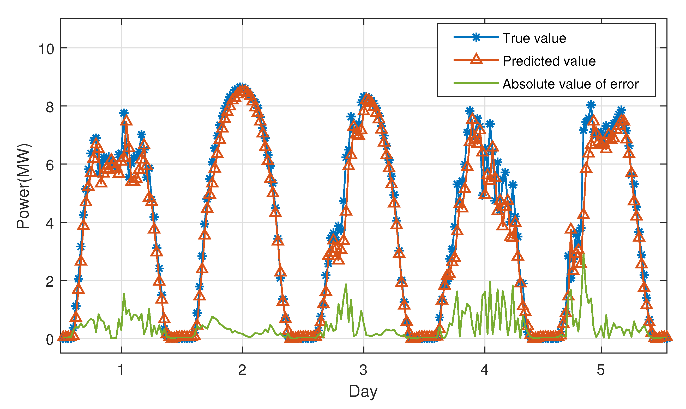
To show the forecasting performance more intuitively and concisely,
Figure 9 illustrates a five-day forecasting curve randomly selected from the testing set. The forecasting value is rather close to the actual value in general. The moment with a large absolute value of error is often the moment when the output power of the PV system is fluctuating. In addition, the more severe the fluctuation, the more unpredictable the forecast; the smoother the output power, the smaller the error.
Fve error types of proposed model are compared with other three contemporary prediction models, including BPNN, general regression neural network (GRNN), and linear regression (LR), in order to fully validate the performance of the proposed PV forecasting model based on RBF neural network.
Figure 10 presents the comparison of the five type of errors on testing set among the proposed approach and the other three methods. With the same input data and training set, the errors of four methods differ. For comparison, the scales of MBEs and MSEs are adjusted in
Figure 10.
Although the MBE of the proposed model is greater than other models, which merely indicates the total bias on testing set is larger than other models, the MAE, MAPE, MSE, and RMSE of proposed forecasting model are superior to those of the other models. Because the comparison is conducted on a testing set, the satisfied performance of proposed model on both forecasting accuracy and robustness is revealed similarly.
4.3. Applicability Analysis of the Model in Four Generalized Weather Types
The forecasting models from four general weather types are discussed in [
29,
43,
44], while the PV power ultra-short-term forecasting model that is proposed in this paper does not distinguish different weather types. To quantify how well the forecasting performance of the forecasting model under different weather conditions is, this section analyzes the applicability of the forecasting performance of the model for different weather types.
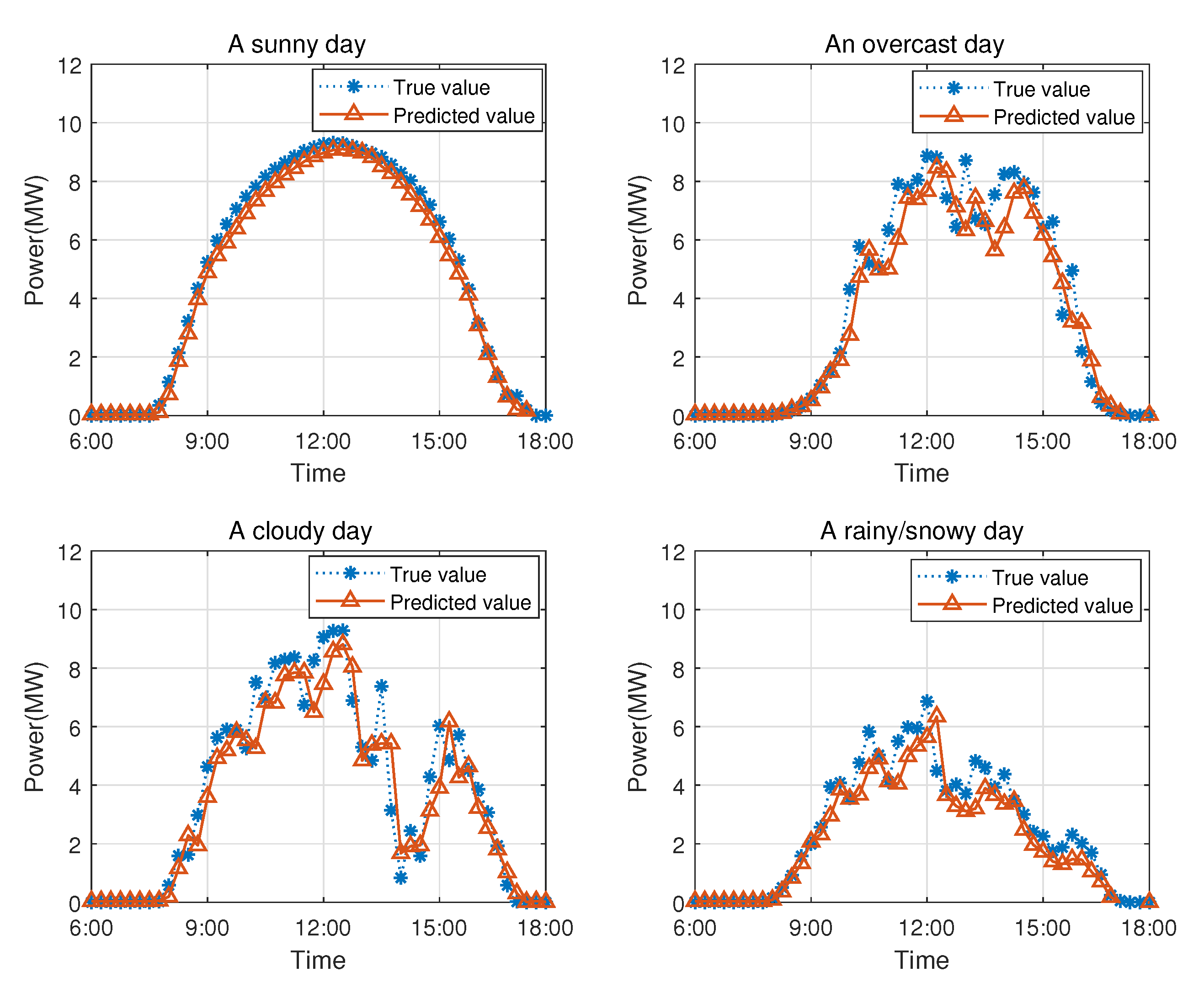
From the test set that is not involved in model training and verification, samples in four generalized weather types are collected.
Figure 11 shows the comparison of the forecasting curves.
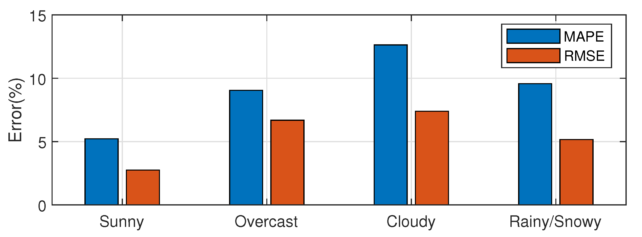
The comparison of the two error types under the four generalized weather types is shown in
Figure 12, and the specific error values are shown in
Table 2.
From
Figure 12 and
Table 2, it can be seen that the forecasting error in the sunny type is the smallest, while, in the remaining three, weather conditions are larger.
On the sunny day, the weather conditions are relatively stable, and the change in solar irradiance over time is relatively smooth and less fluctuating. The autocorrelation of the PV power time series is the strongest. For the RBF network, the output and input data in this case are highly correlated; therefore, the proposed forecasting model can reflect the tendency of the PV power generation accurately.
In cloudy, overcast, and rainy/snowy weather, the cloud covering the PV power plant often changes sharply, thus the fluctuation of solar irradiance in a short period of time is relatively considerable. The autocorrelation of the PV power time series is weak, so the forecasting effect is poor.
Figure 11 shows the fluctuations of power generation during these four days. Obviously, the amount of power generation changes most gently on a sunny day and most dramatically on a cloudy day, which corresponds to the difference in error values over four days, as mentioned above. As the degree of fluctuations of weather types increases, the forecasting accuracy of the ultra-short-term forecasting model gradually decreases. Although the error of the forecasting model is relatively large for some days with fluctuating power generation, the forecasting performance of the model is, in general, still excellent.
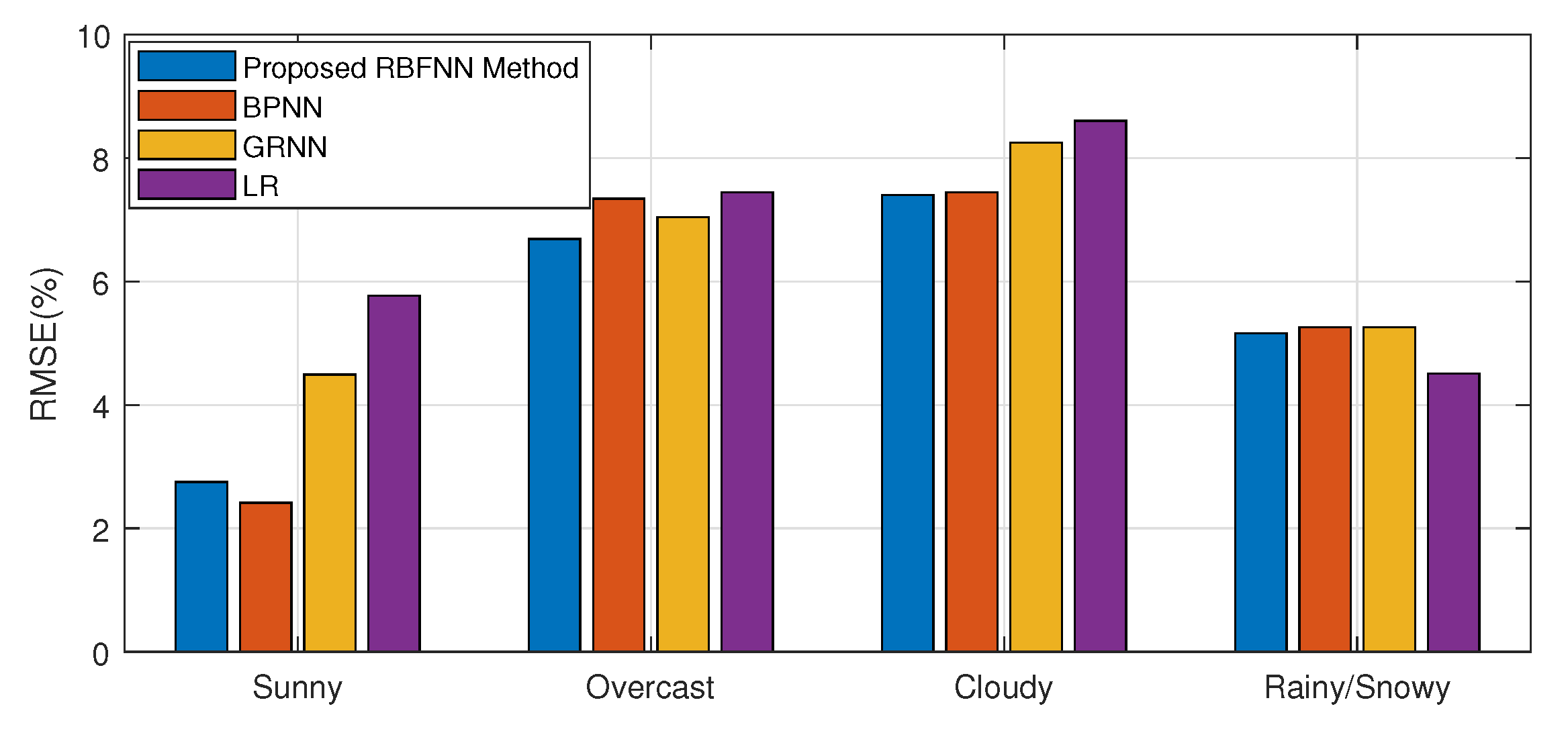
To further evaluate the performance of the proposed model, the comparisons of MAPEs and RMSEs of each model in each weather types are provided in
Figure 13 and
Figure 14, separately. The figures show that the proposed model remarkably outperforms other three ultra-short-term PV power prediction models in most of four seasons, although, in sunny day, the RMSE of BPNN is slightly lower, and in rainy or snowy day, the LR method performs marginally better with respect to MAPE and RMSE.


