Attention Collaborative Autoencoder for Explicit Recommender Systems

Abstract

Recently, various deep learning-based models have been applied in the study of recommender systems. Some researches have combined the classic collaborative filtering method with deep learning frameworks in order to obtain more accurate recommendations. However, these models either add additional features, but still recommend in the original linear manner, or only extract the global latent factors of the rating matrices in a non-linear way without considering some local special relationships. In this paper, we propose a deep learning framework for explicit recommender systems, named Attention Collaborative Autoencoder (ACAE). Based on the denoising autoencoder, our model can extract the global latent factors in a non-linear fashion from the sparse rating matrices. In ACAE, attention units are introduced during back propagation, enabling discovering potential relationships between users and items in the neighborhood, which makes the model obtain better results in the rating prediction tasks. In addition, we propose how to optimize the training process of the model by proposing a new loss function. Experiments on two public datasets demonstrate the effectiveness of ACAE and its outperformance of competitive baselines.

1. Introduction

As an effective tool of information filtering, recommender systems play a significant role in many web applications, such as online shopping, e-commercial services, and social networking applications. Based on predictions of user preferences, recommender systems enables users to find products and contents that are of most interest to them. As a technique commonly used in recommender systems, collaborative filtering (CF) is a predictive process that is based on the similarity of users measured from the historical interaction data, assuming that similar users display similar patterns of rating behavior and that similar items receive similar ratings.

Generally, there are three types of CFs: neighborhood-based models, latent factor models, and hybrid models [1]. For generating recommendations, neighborhood-based models exploit the previous interaction history in order to identify groups or neighborhoods of similar users or items. Latent factor models, such as Matrix Factorization (MF) [2], have been extensively and effectively used to map each user and item of the rating matrices into a common low-rank space to capture latent relations. Neighborhood-based models capture local structures of interaction data by selecting the top-K most relevant users or items, while usually ignoring most of the remaining ratings. By contrast, latent factor models are proficient in capturing overall relationships among users or items, but omits some local strong relationships. The weaknesses of these two models inspire the development of hybrid models, such as Factorization Machines [3] and SVD++ [1], which integrate some neighborhood features, such as users’ historical behaviors and items’ average purchase prices to obtain better prediction results. However, these traditional CF methods are usually in a linear manner and they cannot fully explore the potential information that is contained in the interaction matrices.

Thanks to the excellent performance of deep learning in computer vision [4], machine translation [5], and many other fields, scholars become interested in applying deep learning methods to recommendation tasks. One way is to use a deep learning network to extract hidden features from auxiliary information such as user profiles, item descriptions and knowledge graphs, and integrate them into the CF framework to obtain hybrid recommendations [6,7]. However, this type of model may not be able to find non-linear relationships in the interaction data, because they are essentially modeled linearly in an inner product way as in the MF model. Another way is to model the interaction data directly [8,9] so as to extract nonlinear global latent factors of user preferences, and may help discover more behaviors, which are, however, sometimes incomprehensible behaviors. For instance, Collaborative Filtering Network (CFN) [8] applies the structure of a denoising autoencoder (DAE) [10] in order to construct a non-linear MF from sparse inputs and side information. The Neural Collaborative Autoencoder (NCAE) [9] utilizes the greedy layer-wise pre-training strategy to deal with the difficulty of training a deeper neural network under sparse data. The above models extract the hidden features in a nonlinear fashion and achieve good performance for explicit feedback; however, they do not take the local user-item relationships into account. In other words, they treat all of the rating prediction errors of different users or items indiscriminately and do not put more weights on some local active users whose ratings are more credible. Therefore, by only capturing the global latent factors of the interaction data and ignoring local potential relationships of some active users or popular items, the direct modeling method may not be able to yield very accurate predictions. To focus on the prediction errors of some special users or items, we consider the attention mechanism that widely used in other domains. The attention mechanism essentially focuses on limited attention to key information. It is similar to a method of reweighting to make the model focus on some important parts, such as active users or popular products. Accordingly, we introduce attention mechanism in the direct modeling method in order to discover local structure of user-item matrices for better rating predictions.

In this paper, we propose a novel neural network model called Attention Collaborative Autoencoder (ACAE) for explicit feedback by introducing attention units into a DAE. Our model can be roughly divided into two processes: sparse forward propagation and attention backward propagation. During forward propagation, we carry on a preprocessing on the sparse input vectors, which, on the one hand, greatly reduces the complexity of training the model and, on the other hand, makes the model more robust to learn features. During back propagation, we use the attention units to calculate the credibility of different users or items to obtain some local relationships, so that the model can more accurately calculate the error in order to improve rating predictions. Our main contributions can be summarized, as follows:

• Based on the DAE, a new neural network model is proposed for explicit feedback, called ACAE, which is in a non-linear fashion to explore the interaction matrices. With attention units, it can both capture the global potential relationships and local latent factors between users and items.
• A new loss function for ACAE is designed and a calculation technique is proposed in order to optimize the training process.
• Experiments on two public datasets demonstrate the effectiveness of ACAE in the rating prediction tasks.

The remainder of this paper is organized, as follows. In Section 2, we review some related work on autoencoders applied in recommendation systems and the attention mechanism. We formalize our problem and introduce the basic notations in Section 3. A new framework ACAE and its implementation are presented in the details in Section 4. In Section 5, experimental results on two datasets show the effectiveness and outperforming of our proposed framework. In the end, we conclude our work in Section 6.

2. Related Work

Autoencoders [4], as a kind of feed-forward neural networks, are often applied to extract low-dimensional feature representations from the original data. Recently, more scholars have chosen autoencoders as deep learning frameworks for recommender systems. As an alternative to the traditional linear inner product techniques, autoencoders are suitable to decompose the rating matrices in a non-linear way. For example, Sedhain et al. [11] use an autoencoder to get reconstruction data directly as rating predictions by decomposing a rating matrix, and obtains competitive results on numerous benchmark datasets. Based on a stacked DAE, Wang et al. [6] propose a hierarchical Bayesian model to perform deep representation learning for the content information. To tackle the cold-start problem, Strub et al. [8] utilize a special DAE to deal with sparse data and auxiliary information. Zhang et al. [12] generalize the original SVD₊₊ [1] with a contrastive autoencoder, utilizing auxiliary content information to enrich the hidden features of items.

As a recent trend in deep learning, attention mechanisms are first applied in image recognition. Mnih et al. [13] present a novel RNN model with an attention mechanism that reduces the costs of computing large images. In the field of natural language processing (NLP), Bahdanau et al. [14] propose an approach while using attention mechanisms on machine translation tasks to simultaneously translate and align words. Vaswani et al. [15] replace the recurrent layers most commonly used in encoder-decoder architectures with multi-headed self-attention on machine translation to greatly reduce the training time. Furthermore, the attention mechanism also has played a role in various tasks of recommender systems. For click-through rate prediction, Zhou et al. [16] design a novel model with an attention mechanism for activating related user behaviors and obtaining an adaptive representation vector for user interests, which varies over different ads. For multimedia content, Chen et al. [17] first exploit an attention mechanism combined CF models to discover item-level and component-level implicit feedback to obtain a better multimedia recommendation. For knowledge-aware recommendation, Wang et al. [18] propose a novel graph neural network with an attention mechanism to explore high-order connectivity with semantic relations in a collaborative knowledge graph. Ma et al. [19] have used attention modules to process additional contextual information in their autoencoders and achieve good results in a content-aware recommendation for implicit feedback. Although our model is only appropriate for explicit feedback, ACAE can better handle a rating prediction problem with special attention units and do not need to use additional information.

3. Symbolic Notations

In this section, let us introduce some basic notations.

In collaborative filtering (CF), we have M items, N users, and a partially observed interaction matrix $\mathbf{R}={\left[r_{ij}\right]}_{M\times N}$, where each entry $r_{ij}$ means the rating given by user j for item i. For different datasets, $r_{ij}$ may have different ranges and a commonly used range is from 0.5 to 5. The row and column of the rating matrix $\mathbf{R}$ are written as ${\mathbf{v}}_i$ and ${\mathbf{u}}_j$. And we denote by ${\tilde{\mathbf{v}}}_i$ and ${\tilde{\mathbf{u}}}_j$ the corrupted versions of ${\mathbf{v}}_i$ and ${\mathbf{u}}_j$, respectively, where some observed values in ${\tilde{\mathbf{v}}}_i$ and ${\tilde{\mathbf{u}}}_j$ are dropped out randomly. In addition, the dense estimates of ${\mathbf{v}}_i$ and ${\mathbf{u}}_j$ by the model are written as ${\widehat{\mathbf{v}}}_i$ and ${\widehat{\mathbf{u}}}_j$.

For the neural network that is discussed in our work, we use l to represent the l-th layer. The bias vector and the weight matrix of the l-th layer are denoted as ${\mathbf{b}}^l\in {\mathbb{R}}^{D_l}$ and ${\mathbf{W}}^l\in {\mathbb{R}}^{D_l\times D_{l-1}}$, where $D_l$ represents the hidden dimension. We also use ${\mathbf{W}}^{+}$ to denote a collection of all weight matrices and bias vectors. The activation function for each layer l is denoted by ${\sigma }^l$. For our model, we choose tanh(·) as an activation function for each layer l.

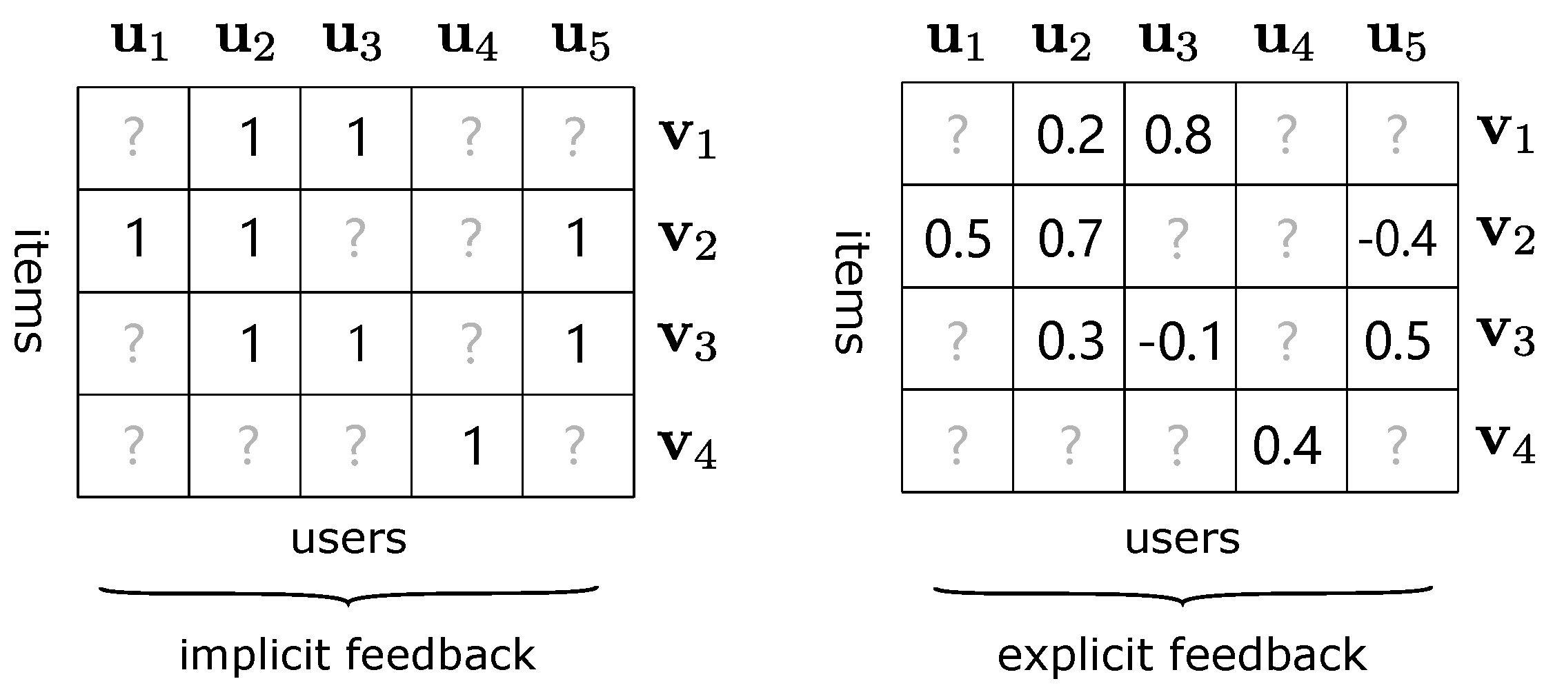
Figure 1 displays two types of feedback. For implicit feedback, it is concerned with whether the user operates on the item, such as rating, browsing, or clicking. In the corresponding interaction matrices, 1 means that the user has performed a certain operation on the item and 0 means not. For explicit feedback, each value in interaction matrices represents the user’s specific rating for the item. We preprocess the original ratings of explicit feedback, as shown in Figure 1, which will be discussed in the details in Section 5. When compared with implicit feedback, the explicit one can better reflect user preferences for some specific items, and it is more suitable for rating prediction tasks, so this paper mainly discusses explicit feedback.

4. Attention Collaborative Autoencoder

In this section, we first introduce the overall framework of our model Attention Collaborative Autoencoder (ACAE). After that, two important processes are introduced in detail: sparse forward propagation and attention backward propagation. In addition, we present a new loss function and adopt a programming technique in order to optimize the training process of our model.

4.1. The Overall Structure of ACAE

An autoencoder [4] is a type of feed-forward neural network, which is trained to encode the input into some representation, such that the input can be reconstructed from such a representation. It can be simple divided into two parts:

$$encoder:f\left(\mathbf{x}\right)=\sigma ({\mathbf{W}}_{\mathbf{1}}\mathbf{x}+{\mathbf{b}}_{\mathbf{1}}),decoder:g\left(\mathbf{y}\right)=\sigma ({\mathbf{W}}_{\mathbf{2}}\mathbf{y}+{\mathbf{b}}_{\mathbf{2}}).$$

(1)

A denoising autoencoder (DAE) is a variant of an autoencoder that is trained to reconstruct the original input from the corrupted form, which makes the network more stable and robust. An important task in collaborative filtering is rating prediction. In the rating prediction task, given an item i and a user j, we need to predict a specific rating $r_{ij}$ in an interaction matrix $\mathbf{R}$. For a DAE, the rating prediction problem in CF can be formalized as: a process of transforming the sparse corrupted vector ${\tilde{\mathbf{v}}}_i$ and ${\tilde{\mathbf{u}}}_j$ into dense vector ${\widehat{\mathbf{v}}}_i$ and ${\widehat{\mathbf{u}}}_j$, respectively.

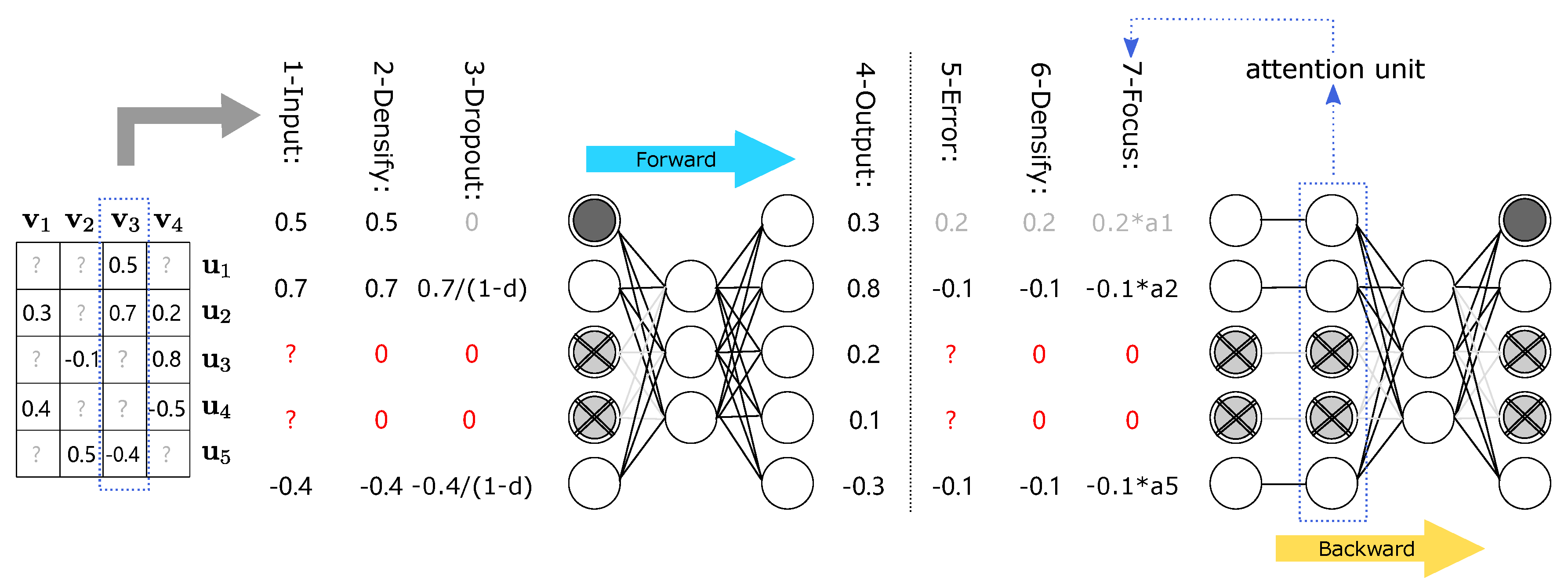
Selecting the DAE as basic network architecture, our model ACAE, as illustrated Figure 2, contains one hidden layer and one output layer, and can be formulated, as follows:

$${\widehat{\mathbf{v}}}_i=nn\left({\tilde{\mathbf{v}}}_i\right)=\stackrel{dec}{\overbrace{{\sigma }^2({\mathbf{W}}^2\underset{enc}{\underbrace{\left({\sigma }^1({\mathbf{W}}^1{\tilde{\mathbf{v}}}_i+{\mathbf{b}}^1)\right)}}+{\mathbf{b}}^2)}},$$

(2)

where the first layer ${\sigma }^1(·)$ of ACAE is an encoding part and the second one ${\sigma }^2(·)$ is a decoding part. The encoder ${\sigma }^1(·)$ builds a low-rank dense form of input $\tilde{\mathbf{v}}$ and the decoder ${\sigma }^2(·)$ predicts a dense rating vector $\widehat{\mathbf{v}}$ from the encoder.

There are generally two types of autoencoders, depending on different ways to handle the interaction matrices: user-based and item-based [11,20], while the latter one yields a better performance on recommender systems with explicit feedback as described in [8]. Accordingly, in the current work, we only consider the item-based autoencoder, but our method also applies to the user-based one.

In the sequel, we will describe two important processes of ACAE in the details.

4.2. Sparse Inputs during Forward Process

For CF-based recommender systems, a big challenge is the sparsity problem and it is common that more than $90\%$ of values are missing in some datasets. When training in CF, these unknown missing values make the task even more difficult. One solution is to use the Word Embedding that converts sparse vectors into dense vectors, in order to obtain potentially low-dimensional information. Another method is to integrate extra side information into the original inputs. We try to let the autoencoder solve the prediction problem by itself.

During the forward propagation of ACAE, we have to take some measures to deal with the sparse input vector ${\mathbf{v}}_i$. One important step is to assign unobserved ratings in input vectors to zero, which greatly reduces the complexity of model training. Subsequently, unlike in the DAE, we only randomly discard observed input units, which means that the ACAE needs not only to reconstruct new ratings for discarded data, but also to predict new ratings for those data that are not discarded. Through the previous step, our model can own a more robust feature learning capability. We take the network in Figure 2 as an example in order to understand this process more vividly. For the input vector ${\mathbf{v}}_3$, in the third stage, among the non-missing elements $u_1,u_2,u_5$, only $u_1$ is selected to be discarded.

In fact, the vector ${\tilde{\mathbf{v}}}_i$ obtained after discarding is the real input of ACAE, which is used to learn potential relationships between different items. In order to obtain the real input ${\tilde{\mathbf{v}}}_i$, we choose dropout as the discarding strategy. Unlike using dropout as a regularization method, we only use it for the observed vectors on the input layer. For each epoch, the observed vector ${\mathbf{v}}_i$ is randomly discarded independently with a probability d. In order to make the corrupted vector ${\tilde{\mathbf{v}}}_i$ unbiased, values of ${\tilde{\mathbf{v}}}_i$ need to be scaled by $1/(1-d)$, which are not dropped out. An element $\tilde{x}$ in the real input ${\tilde{\mathbf{v}}}_i$ can be written, as follows:

$$\tilde{x}=\left\{\begin{array}{cc}0\hfill & \mathrm{if}x\mathrm{is}\mathrm{dropped},\hfill \\ \frac{x}{(1-d)}\hfill & \mathrm{if}x\mathrm{is}\mathrm{not}\mathrm{dropped},\hfill \end{array}\right.$$

(3)

where x represents a original value in the observed vector ${\mathbf{v}}_i$.

After the above steps, the real input vector ${\tilde{\mathbf{v}}}_i$ needs to go through the encoding part and the decoding part of the model ACAE. For the encoding part, we only need to forward the non-zero values in the input vector ${\tilde{\mathbf{v}}}_i$ with the corresponding columns of ${\mathbf{W}}^1$:

$$encoder:{\mathbf{z}}_i^1={\sigma }^1({\mathbf{W}}^1{\tilde{\mathbf{v}}}_i+{\mathbf{b}}^1),$$

(4)

where ${\mathbf{z}}_i^1$ represents the output of the encoding part. For our model, ${\mathbf{z}}_i^1$ is actually a low-dimensional representation of input vector ${\tilde{\mathbf{v}}}_i$. As displayed in the left of Figure 2, only ${\tilde{\mathbf{v}}}_{32}$ and ${\tilde{\mathbf{v}}}_{35}$ are forwarded with their linking weights. In order to obtain the final dense vector ${\widehat{\mathbf{v}}}_i$, we use ${\mathbf{z}}_i^1$ as the input of the decoding part:

$$decoder:{\widehat{\mathbf{v}}}_i={\sigma }^2({\mathbf{W}}^2{\mathbf{z}}_i^1+{\mathbf{b}}^2).$$

(5)

In the decoding part, the latent low-rank representation ${\mathbf{z}}_i^1$ is then decoded back to predict the dense ${\widehat{\mathbf{v}}}_i$ during inference.

4.3. Attention Units during Backward Process

Most direct modeling methods learn the global latent factors through the rating matrices, and usually do not consider the local features of users or items. Because they treat each user or item of prediction errors equally during back propagation, which ignores the influence of some active users or popular items in the neighborhood. Without extra operations, this direct modeling manner cannot fully explore latent relationships in the interaction data. Accordingly, we add attention units to focus on some local features of the interaction data.

During back propagation, we also assign prediction errors of missing values to zero, which corresponds to a similar operation of us in the forward process. In fact, these prediction errors of missing values cannot bring useful information. If we do not discard these errors of missing values, they will make our model tend to predict all ratings as zero. Because these miss values have been converted to zero in the forward process and the interaction matrix $\mathbf{R}$ is quite sparse. Subsequently, we introduce attention units to reallocate other prediction errors of non-missing values, which enables ACAE to capture local relationships between active users and popular items in the neighborhood. We give a simple example in order to explain the importance of these active users or popular items. The user ${\mathbf{u}}_3$ rates five items and the user ${\mathbf{u}}_1$ only rates one in the neighborhood, as displayed in the Figure 3. It is unfair to treat prediction errors of user ${\mathbf{u}}_3$ and user ${\mathbf{u}}_1$ in the same way, because ratings of user ${\mathbf{u}}_3$ are more credible. So, user ${\mathbf{u}}_3$ needs more attention than the user ${\mathbf{u}}_1$. In fact, these are the active users we need to pay more attention to. Their ratings are more valuable, but some direct modeling methods often ignore these users. For items, they still have the same situations. Formally, we define the item/user’s contributions or attentions, as follows:

$$c\left({\mathbf{v}}_i\right)=\frac{\left|K\right({\mathbf{v}}_i\left)\right|}{\left|F\right({\mathbf{v}}_i\left)\right|},c\left({\mathbf{u}}_j\right)=\frac{\left|K\right({\mathbf{u}}_j\left)\right|}{\left|F\right({\mathbf{u}}_j\left)\right|},$$

(6)

where $K\left({\mathbf{v}}_i\right)$ is a index set for observed elements of ${\mathbf{v}}_i$, and $F\left({\mathbf{u}}_j\right)$ is a index set for all elements of ${\mathbf{u}}_j$. We take the user ${\mathbf{u}}_1$ in the Figure 3 as an example, $K\left({\mathbf{u}}_1\right)=\left\{2\right\}$ and $F\left({\mathbf{u}}_1\right)=\{1,2,3,4,5\}$. Because the rating matrices are too sparse, we ignore the impacts of concrete rating values in vectors. For attention units, it is more important whether users rate an item rather than knowing what the specific score is.

This neural attention strategy learns an adaptive weighting function to focus on influential items/users within the neighborhood to produce more reasonable rating predictions. Because the observed input data of ACAE are randomly dropped at each iteration, the attentions of items/users are different each time. It is still unreasonable to use these attention values directly. We also have to consider the possible impact between all items/users in the neighborhood. Formally, we compute the attention weights for an item or a user to infer the importance of each item’s or user’s unique contribution to the neighborhood:

$$a_i=\frac{exp\left(c\left({\mathbf{v}}_i\right)\right)}{{\sum }_{k\in I\left(i\right)}exp\left(c\left({\mathbf{v}}_k\right)\right)},a_j=\frac{exp\left(c\left({\mathbf{u}}_j\right)\right)}{{\sum }_{k\in U\left(j\right)}exp\left(c\left({\mathbf{u}}_k\right)\right)},$$

(7)

where $I\left(i\right)$ represents the index set of items in the same neighborhood as item i and $U\left(j\right)$ represents the index set of users in the same neighborhood as user j. This attention strategy produces a distribution over the neighborhood and makes the model focus on or place higher weights on some distinctive users or items in the neighborhood.

Finally, we want to combine two types of attention in order to produce a final neighborhood attention value:

$$a_{ij}=\gamma ·(a_i·a_j),$$

(8)

where $\gamma$ is an initial attention value that can control the importance of errors to our model. Additionally, $a_{ij}$ can be simply explained that how much impact the model has by the rating operation of user j to item i during back propagation.

4.4. New Loss Function

The right half of the Figure 2 displays a simple example of ACAE’s back propagation. For the item ${\mathbf{v}}_3$, the missing $u_3$ and $u_4$ are ignored, and the prediction errors of ${\mathbf{v}}_3$ is calculated as: $\{{\mathbf{v}}_{3j}-nn{\left({\tilde{\mathbf{v}}}_3\right)}_j\}$, the same process for ${\mathbf{v}}_1$, ${\mathbf{v}}_2$ and ${\mathbf{v}}_4$. When non-missing errors pass through attention units, they are dynamically reweighted according to their attentions. This process makes ACAE pay more attention to those special items and users in the neighborhood, instead of treating them in the same way. Like the DAE loss function, we also introduce two hyperparameters, $\alpha$ and $\beta$, into our new loss function to balance prediction errors and reconstruction errors. In addition, we utilize attention values in loss function in order to emphasize different effects of the users/items in the current neighborhood:

$$L_{2,\alpha ,\beta }({\mathbf{v}}_i,{\tilde{\mathbf{v}}}_i)=\alpha (\sum _{j\in G({\mathbf{v}}_i,{\tilde{\mathbf{v}}}_i)}{a}_{ij}\times {[nn{\left({\tilde{\mathbf{v}}}_i\right)}_j-{\mathbf{v}}_{ij}]}^2)+\beta (\sum _{j\notin G({\mathbf{v}}_i,{\tilde{\mathbf{v}}}_i)}{a}_{ij}\times {[nn{\left({\tilde{\mathbf{v}}}_i\right)}_j-{\mathbf{v}}_{ij}]}^2),$$

(9)

where $G({\mathbf{v}}_i,{\tilde{\mathbf{v}}}_i)=K\left({\mathbf{v}}_i\right)\cap C\left({\tilde{\mathbf{v}}}_i\right)$, $K\left({\mathbf{v}}_i\right)$ is a set of the indexes for the observed input ${\mathbf{v}}_i$, and $C\left({\tilde{\mathbf{v}}}_i\right)$ are the indexes for dropped elements of ${\tilde{\mathbf{v}}}_i$. Take Figure 2 as a concrete example to illustrate, $K\left({\mathbf{v}}_3\right)=\{1,2,5\}$ and $C\left({\tilde{\mathbf{v}}}_3\right)=\left\{1\right\}$. Finally, we minimize the following average loss over all of the items to learn the parameters:

$$\mathcal{L}=\frac{1}{M}\sum _{i=1}^M{L}_{2,\alpha ,\beta }({\mathbf{v}}_i,{\tilde{\mathbf{v}}}_i)+\frac{\lambda }{2}\left|\right|{\mathbf{W}}^{+}\left|\right|,$$

(10)

where we use the squared $L2$ norm as the regularization term to prevent our model overfitting.

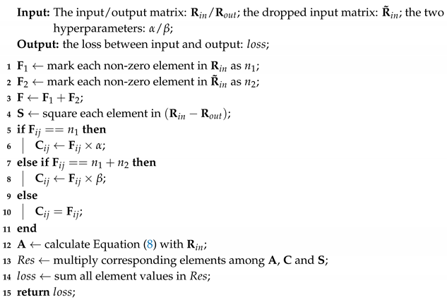
Calculating a loss value is always a time-consuming part of training models. For each item ${\mathbf{v}}_i$, it is necessary to separately calculate every element in its observed set $K(·)$ and corrupted set $C(·)$ during computing the loss function. Additionally, this process often introduces some loop operations that increase the computation time. For the input matrix, we adapt a marking-like method that does not require to compute the loss value of each item one-by-one. The detailed operation process is described in Algorithm 1.

Algorithm 1 explains the main process of calculating the Equation (9), where the $n_1$ and $n_2$ are two integers that are specified by users, the ${\mathbf{F}}_{ij}$ represents an element value in the matrix $\mathbf{F}$. We use two different tags $n_1$ and $n_2$ to locate each element that needs to multiply by $\alpha$ or $\beta$. Through the $tf.where(·)$ function in the TensorFlow (https://www.tensorflow.org), we do not require to use a loop to compute each element one by one in the corresponding set, which optimizes the training process of ACAE.

Algorithm 1: The calculation process of the new loss function.

5. Experiments

In this section, we first introduce two datasets, and then list some baselines and implementation details, and finally compare and analyze some relevant experimental results.

5.1. Datasets

To demonstrate the effectiveness of ACAE, we use two publicly available datasets, the MovieLens 1M (https://grouplens.org/datasets/movielens/1m) and 10M (https://grouplens.org/datasets/movielens/10m). MovieLens are a series of datasets on movie ratings and ratings there in scale from 0.5 to 5.

Table 1. Statistics of Datasets.

Dataset	#Users	#Items	#Ratings	Density
ML-1M	6040	3706	1000209	4.47%
ML-10M	69878	10677	10000054	1.34%

summarizes the detailed descriptions of these two datasets.

As in [8], we make a preprocessing on these datasets and randomly divide each dataset into 80%–10%–10% training-validation-test sets. Moreover, all of the ratings in the datasets are normalized into values between $-1$ and 1. Next, we make the inputs unbiased by setting $r_{ij}^{unbiased}=r_{ij}-b_{v_i}$, where $r_{ij}$ is a original rating and $b_{v_i}$ is the mean of the i-th item. Later, we will add back the bias calculated on the training set when evaluating the learning matrix.

5.2. Implementation Details and Baseline

Training Settings. Our model ACAE is implemented through Python and TensorFlow. For the network, we choose the Xavier-initializer in order to initialize the weights and use the tanh(·) as an activation function; the training is carried by Stochastic Gradient Descent with mini-batch of size 256; for optimization, we choose the Adam optimizer and set the learning rate to be 0.001, which can adapt the step size automatically during the training process; other hyperparameters of ACAE are tuned through the grid search method. For each experiment, we all randomly divide each dataset into $80\%$-$10\%$-$10\%$ training-validation-test datasets. Our model is retrained on the training/validation sets and finally evaluated on the test set. We repeat the above process five times and record the average performance.

Evaluation Metrics. The Root Mean Square Error (RMSE) is used to evaluate the prediction performance:

$$RMSE=\sqrt[]{\frac{{\sum }_{(i,j)\in \mathbf{R}}{({\mathbf{R}}_{i,j}-{\tilde{\mathbf{R}}}_{i,j})}^2}{\left|\mathbf{R}\right|}},$$

(11)

where $\left|\mathbf{R}\right|$ is the number of ratings in the test set, ${\mathbf{R}}_{i,j}$ denotes the rating on item i given by user j, and ${\tilde{\mathbf{R}}}_{i,j}$ is the predicted value of ${\mathbf{R}}_{i,j}$. A smaller value of RMSE means better performance.

Baseline Methods. For explicit feedback, we benchmark ACAE with the following algorithms:

• ALS-WR [21] solves a low-rank matrix factorization problem by optimizing only one parameter with others fixed in each iteration.
• SVDFeature [22] is a machine learning toolkit for the feature-based matrix factorization, which wins KDD Cup for two consecutive years.
• LLORMA [23] uses a weighted sum of low-rank matrices to represent an observed matrix, which usually performs best among the conventional methods.
• I-AutoRec [23] trains one autoencoder for each item, sharing the weights between the different autoencoders.
• V-CFN [8] computes non-linear matrix factorization from sparse rating inputs and side information, and it achieves good experimental results.
• NCAE [24] is an outstanding model for explicit feedback and implicit feedback, which is based on a DAE with multi-hidden layers.

In our experiments on MovieLens 1M and 10M, we train an ACAE with only two layers. We set the number k of neural units in the hidden layer to 700, unless otherwise specified. For regularization, we set the weight decay $\lambda$ to $0.1$ and the input dropout ratio d to $0.5$. Additionally, some parameter settings of baselines are the same in the original papers. We compare the experimental results of ACAE with these baselines on the same data splitting procedure (90%–10% training-test).

5.3. Experimental Results

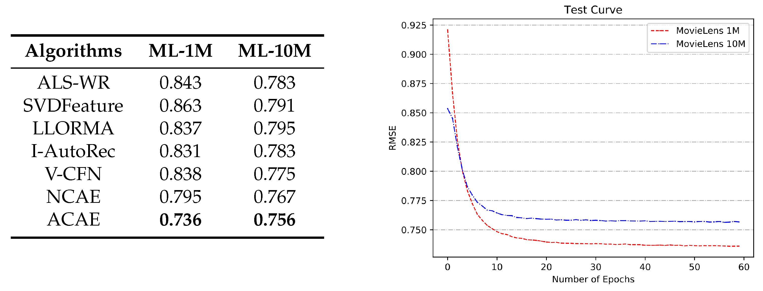
Comparison with Baselines. The left of the Figure 4 shows the performance of ACAE and other baselines on two datasets. First, we can clearly see that ACAE achieves the best results with the RMSE values of $0.736$ and $0.756$ on the MovieLens 1M and 10M, respectively. Second, as compared to classical linear methods, neural network models obtain smaller prediction errors by virtue of their own non-linear ways, such as I-AutoRec, V-CFN, NCAE, and ACAE. Third, even if there is no deeper network structure, our model still achieves better prediction results than NCAE, which verifies the influence of some local neighborhood relationships that were obtained by attention units. Fourth, we can find that LLORMA has better results on the MovieLens 1M than ALS-WR and SVDFeature, but not on the 10M. Observed from that presented in Table 1, the rating density of the MovieLens 1M is $4.47\%$, which is about three times the 10M. This means the neighborhood-based model is easier to discover the potential relationships between users and items on dense datasets. Because of the attention units, our model also appears to be a similar phenomenon to LLORMA and it gets more obvious improvements with the help of the neural network structure. Because the small dataset MovieLens 1M has more dense data, missing ratings have smaller impacts on calculating the attention values of users or items. Accordingly, ACAE can perform better experimental results on the MovieLens 1M.

Then, we analyze the changes in the model during training. The right of the Figure 4 displays two curves of RMSE values on two test sets. Our model ACAE starts to converge on both datasets when the epoch is around 20, and then quickly converges to lower RMSE values. In the first few iterations, the curve of RSME values on the MovieLens 10M has a lower value than that on the 1M. For instance, when the epoch is about 2, ACAE obtains an RMSE value of $0.850$ on the MovieLens 10M and gets a higher value of $0.920$ on the 1M. However, as the number of iteration increases, the RMSE value of ACAE on the MovieLens 10M is gradually higher than that on the 1M. The main reasons for this phenomenon are the following: (1) at the start, ACAE cannot learn parameters well and the attention units have not yet worked. Accordingly, more data at the beginning of training can bring better rating predictions. (2) With the number of epochs increases, for the more dense dataset, attention units can more accurately calculate the attention values of users or items to reweight prediction errors. For these reasons, our model eventually gets a better learning ability and lower RMSE value on the MovieLens 1M. Therefore, we can speculate that ACAE is more suitable for processing a more dense dataset.

Analysis of Model Configurations. For the structure of ACAE, a parameter of great significance is the size of hidden layer units.

Table 2. Test RMSE with varying configurations about size of hidden units on the MovieLens 1/10M.

Hidden Units	ML-1M	ML-10M
300	0.747	0.769
400	0.741	0.764
500	0.739	0.761
600	0.737	0.758
700	0.736	0.756

shows the changes in RMSE values as the size k of hidden layer units increases from 300 to 700 on both of the datasets. We find that increasing the size of hidden layer units can improve the prediction ability of the model. Although as the size of the hidden layer unit increases, the RMSE value of the model’s rating prediction errors begins to decrease. A smaller value of RMSE means better performance. However, the difference between the RMSE obtained with each change is getting smaller and smaller. For example, for the MovieLens 10M, when k is from 300 to 400, the RMSE value is increased by $0.005$. However, when k is from 600 to 700, the RMSE value is only increased by $0.002$. Hence, we finally choose k = 700 as the default size of hidden layer units in the model.

Training Cost. By exploring the training process, the training complexity for one item i is: $O\left(D_1\right|R\left(i\right)|+|R\left(i\right)\left|D_2\right)$, where $D_1$ and $D_2$ are the dimensions of the corresponding layers and $\left|R\right(i\left)\right|$ is the number of observed values for item i. All of our experiments are conducted on a GTX 2080 GPU (Nvidia, Santa Clara, CA, USA). For MovieLens 1M and 10M, we both run 50 epochs and, on average, each epoch costs $0.63$ s and $6.2$ s respectively.

6. Conclusions and Future Work

In this paper, we propose a novel deep learning framework, named ACAE, for explicit recommender systems. With the structure of a DAE, our model can extract the global latent factors in a non-linear fashion from the sparse rating matrices. To obtain better results in the rating prediction tasks, we introduce attention units during back propagation that can discover potential relationships between users and items in the neighborhood. Moreover, we describe a method of computing a new loss function in order to optimize the training process. Experiments on two public datasets demonstrate the effectiveness and outperformance of ACAE as compared to other approaches.

In future work, we will consider how to combine auxiliary information, such as user documentation, product descriptions, and different social relationships, in order to solve the cold-start problem. The other promising direction is to modify the structure of the model to take the historical data into account, so as to further improve the accuracy of rating predictions.