Article

Research and Implementation of Intelligent Decision Based on a Priori Knowledge and DQN Algorithms in Wargame Environment

1
School of Management and Engineering, Nanjing University, Nanjing 210023, China
2
School of Electronics, Computing and Mathematics, University of Derby, Kedleston Rd, Derby DE22 1GB, UK
*
Authors to whom correspondence should be addressed.
Electronics 2020, 9(10), 1668; https://doi.org/10.3390/electronics9101668
Submission received: 28 August 2020 / Revised: 3 October 2020 / Accepted: 6 October 2020 / Published: 13 October 2020
(This article belongs to the Special Issue Deep Reinforcement Learning: Methods and Applications)

Abstract

:
The reinforcement learning problem of complex action control in a multi-player wargame has been a hot research topic in recent years. In this paper, a game system based on turn-based confrontation is designed and implemented with state-of-the-art deep reinforcement learning models. Specifically, we first design a Q-learning algorithm to achieve intelligent decision-making, which is based on the DQN (Deep Q Network) to model complex game behaviors. Then, an a priori knowledge-based algorithm PK-DQN (Prior Knowledge-Deep Q Network) is introduced to improve the DQN algorithm, which accelerates the convergence speed and stability of the algorithm. The experiments demonstrate the correctness of the PK-DQN algorithm, it is validated, and its performance surpasses the conventional DQN algorithm. Furthermore, the PK-DQN algorithm shows effectiveness in defeating the high level of rule-based opponents, which provides promising results for the exploration of the field of smart chess and intelligent game deduction.

1. Introduction

AlphaGo defeated the world Go Chess champion Lee in 2016, which caused a new upsurge of interest in artificial intelligence (AI), especially in the field of game AI. The goal of game AI is not only to let machines play games, but also to simulate real-world operation through game simulation environment [1]. AI researchers can experiments in games and transfer successful AI capabilities to the real-world applications. Although AlphaGo is a milestone in the goal of general artificial intelligence, in general, the problems it represents are still relatively simple compared with the real world [2]. Therefore, in recent years, researchers have focused on real-time strategy (RTS) games [3,4,5,6], such as Dota2 [7] and StarCraft [8,9], which represent dynamic games of asymmetric information beyond the Go game.
To master RTS games, players need strong skills in both macro-strategy operation and micro-execution. In recent studies, micro-level implementation has been the subject of extensive attention and many attempts [10,11,12]. So far, OpenAI has made the latest progress in using Dota2 AI (OpenAI Five) developed by reinforcement learning (RL). OpenAI Five is trained directly in micro-motion space using proximity strategy optimization algorithms and team rewards [13]. OpenAI Five demonstrated stronger team fighting skills and coordination ability than the top professional Dota2 team in the 2018 international competition [7]. The OpenAI approach does not explicitly model macro strategies, but attempts to use a micro-level game to learn the whole game. However, due to the weakness of AI’s macro strategic decision-making ability, OpenAI Five failed to beat the professional teams [14,15]. Although some achievements have been made in RTS games, there are still many difficulties in both OpenAI’s game AI on Dota and Deepmind’s game AI on StarCraft [16,17,18].
On the other hand, a few scholars have studied wargame deduction. Round-robin confrontation is closer to the AI achieved by AlphaGo, and it is easier to solve the problems of micro-strategy modeling and macro-strategy modeling, so it is easier to achieve the AI expected by AlphaGo than RTS games [19,20,21,22].
On this basis, we developed an intelligent game simulation environment, and verified its feasibility through simulated experiments, where a series of basic functional interfaces can be configured to realize the confrontation of different types of operators on different maps. Secondly, this paper uses this platform to verify the feasibility of the DQN (Deep Q Network) algorithm in the field of wargames. The DQN algorithm model combined with prior knowledge (PK-DQN) is established, and the DQN algorithm is optimized to realize the PK-DQN algorithm. Compared with the DQN algorithm, the PK-DQN algorithm has a better convergence effect, is more stable, and has a higher winning rate in the intelligent war game simulation environment. Finally, via simulations, the PK-DQN algorithm is proved to be able to defeat high-level rule-based opponents, which provide an important foundation work for further exploration of deep reinforcement learning in turn-based games.
The value of this article is to use the reinforcement learning algorithm to implement the intelligent AI in turn-based games, in order to explore the feasibility of the reinforcement learning algorithm in wargaming, and we have further improved the DQN algorithm and proposed the PK-DQN algorithm. In addition, we have built a deductive antagonism environment independently, which provides a good basis for future research on reinforcement learning algorithms in wargames. Of course, in this field, the current research still faces many difficulties to overcome in practical application, such as rules and evaluation of closed-domain problems, robustness problems, algorithm migration problems, and the problem of countering scene complexity, which are all the difficulties that existing research needs to solve when applied in practice.

2. Intelligent Decision-Making Model of Tactical Wargame Based on Q-Learning

Through in-depth analysis of the Q-learning method, the intelligent decision-making model of tactical wargame based on Q-Learning was initially implemented to provide basis for the construction of intelligent wargames.

2.1. The Principles of Q-Learning

We create a table where you can calculate the expectation of the maximum future reward for each action in each state. Based on this table, we can calculate the best action for each state. This is supposed to have six directions of movement, and another static state. So we designed a total of seven states of 6 + 1, including East, West, Northeast, Northwest, Southeast, Southwest, and Stationary. Therefore, each piece of land is surrounded by six pieces of land, and one is still, which adds up to seven states, as shown in Figure 1. The 1811 grid marked with the red in Figure 2 represents the reward value of each action of tank 1 moving southwest. The 1712 grid marked with the blue represents the reward value for each move tank 1 makes to the East. Tank 1 is blocked by tank 2 when it moves Southeast, so it cannot be moved. Furthermore, there is no return value for different actions of 1812 coordinates in the southeast, so it is indicated by “-”.
During the calculation, we can convert the grid into a table.
This form is called q-table (Q stands for the “quality” of the action). Each column will represent seven operations (East, West, Northeast, Northwest, Southeast, Southwest, and Stationary), with rows representing states. The value in each cell represents the maximum future reward expectation for a given state and a corresponding action. The score of each q-table will represent the maximum expectation of future reward obtained by taking corresponding actions under the given optimal strategy. Each value in the q-table is obtained using the Q-learning algorithm.
The action value function (or Q function) has two inputs: state and action. It will return for future reward expectations for performing the action in that state.
Q π ( s , a ) = E π [ r t + 1 + γ r t + 2 + γ 2 r t + 3 + | A t = a , S t = s ]
where the sum of rewards r t discount by γ at each time step t ,   γ is a decay factor that represents how much future returns affect the current situation, γ is the decay value used to control the effect of future return on Q. The closer γ is to 1, the more forward-looking it will be as it focuses on the value of subsequent states. When γ approaches 0, it will become more focused on the impact of current interests. So for γ from 0 to 1, the algorithm will increasingly consider the impact of subsequent returns. Achievable by a behavior policy π = P ( a | s ) , after making an observation(s) and taking an action(a). In other words, it can give every action a score as a evaluation, but the future is full of randomness, anything can be happen. Therefore the Q function cannot give you a definite answer, it can only tell you the expectation, so the cumulative reward of the state-action can be expected by subsequent states. Expectation is like an average; it is the return you expect to see. The reason we use expectation is that when you reach a state, there will be some random events. You may have a random strategy, which means we need to combine the results of all the different actions we take. In addition, the transition function can be random, that is, we may not end any state with 100% probability. When an action is selected, the environment returns to the next state. Even if an action is given, there may be multiple status returns. All these random factors are expected to be taken into account. In the simulation experiment, a reward value is calculated for each step, and the next action is selected according to the size of the reward value. Generally speaking, we choose the action that corresponds to the maximum reward value, which is Q*.
The general idea of intelligent decision-making modeling of tactical wargame based on Q-Learning is described above, but there are still significant problems in using the algorithm of Q-learning to build intelligent wargames. Although the Q-learning method can provide basic ideas for the construction of intelligent wargame, the traditional table form stores the state and corresponding Q-value to find the best executive action. But in the case of a too complex state, the computer memory is limited, it is difficult to achieve all storage, and it is also time-consuming work to search all tables. Therefore, this paper further considers whether the improved DQN algorithm can be used to realize the behavior decision-making modeling of intelligent wargames.

2.2. Deep Q Network (DQN)-Based Behavior Decision-Making Model of Intelligent Wargames

This paper first tries to use Q-learning to discover big problems in the process, and then tries to use the DQN algorithm to model the behavior decision-making of intelligent wargames. Based on the analysis of the DQN algorithm, an intelligent wargame model of the DQN algorithm is established, and the intelligent wargame based on the DQN algorithm is successfully implemented.
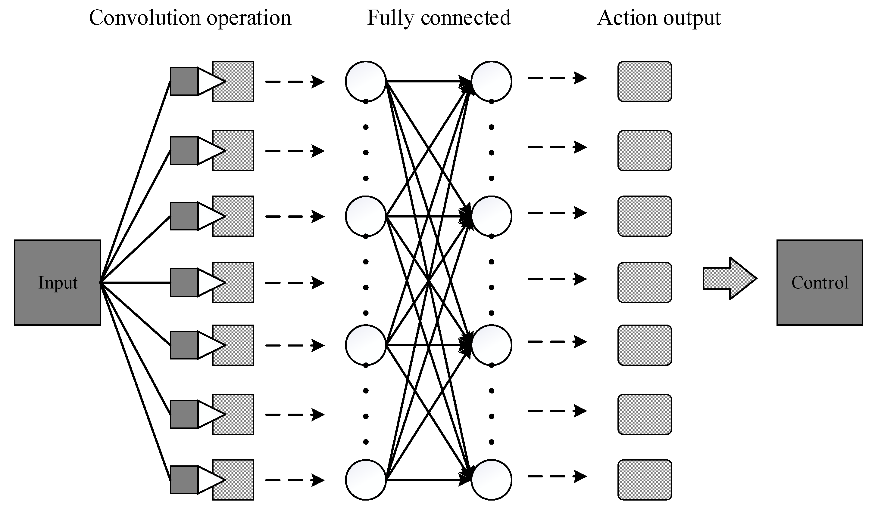
DQN is an intelligent algorithm that combines deep learning with reinforcement learning. It mainly uses deep learning to take state and action as input values of the neural network. After the analysis of the neural network, it gets the Q-value, so it is unnecessary to record the Q-value in the table, and directly uses a neural network to generate the Q-value. Then, it uses the correct Q value provided by reinforcement learning and the Q-value to calculate the loss function, so as to improve the network weight of deep-learning models. According to the output action value of the neural networks and the principle of Q-learning, the method directly selects the action with the maximum value as the next action to be done. It integrates the neural network and Q-learning method, namely the DQN algorithm, the framework is shown in Figure 3.
DQN initializes the memory library first, and assigns random weights to each target Q value, initializes the queue according to each episode. It randomly selects an action with epsilon (epsilon is a parameter that controls the probability of random exploration). Otherwise, it selects the action with the largest Q value with epsilon 1-epsilon to perform this action, observes the return value and the next state, updates the state, action and next round, and updates the state, action, return, and next state. It saves the transition, then extracts samples from the transition using sample to learn, and then updates the calculated Q value until the end of the round. It uses Q value to reverse update the parameters of neural network, and are continuously tuned until the end. It adds the section in 7. It employs just trial and error to store the data. Next, the data is stored to a certain extent, and each time the data are randomly used, the gradient decreases. See the Appendix B for a detailed explanation of the algorithm.
The Algorithm 1 is as follows:
Algorithm 1: Deep Q-learning with experience in reply.
Initialize reply memory D to capacity N
Initialize action-value function Q with random weights θ
Initialize target action-value function Q with weights θ = θ
For episode = 1, M do
  Initialize sequence s 1 = { x 1 } and preprocessed sequence ϕ 1 = ϕ ( s 1 )
  For t = 1 , T do
    With probability ε select a random action a t
    Otherwise select a t = a r g m a x a Q ( ϕ ( s t ) , a ; θ )
    Execute action a t in emulator and observe reward r t and image x t + 1
    Set s t + 1 = s t ,   a t ,   x t + 1 and preprocess ϕ t + 1 = ϕ ( s t + 1 )
    Store transition ( ϕ t ,   a t , r t , ϕ t + 1 ) in D
    Sample random minibatch of transitions ( ϕ j ,   a j , r j , ϕ j + 1 ) from D
    Set y j = { r j ,   i f   e p i s o d e   t e r m i n a t e s   a t   s t e p   j + 1 r j + γ m a x a Q ^ ( ϕ j + 1 , a ; θ ) ,   o t h e r w i s e
    Perform a gradient descent step on ( y j Q ( ϕ j , a j ; θ ) ) 2 with respect to the network parameter θ
    Every c steps reset Q ^ = Q
  End For
End For
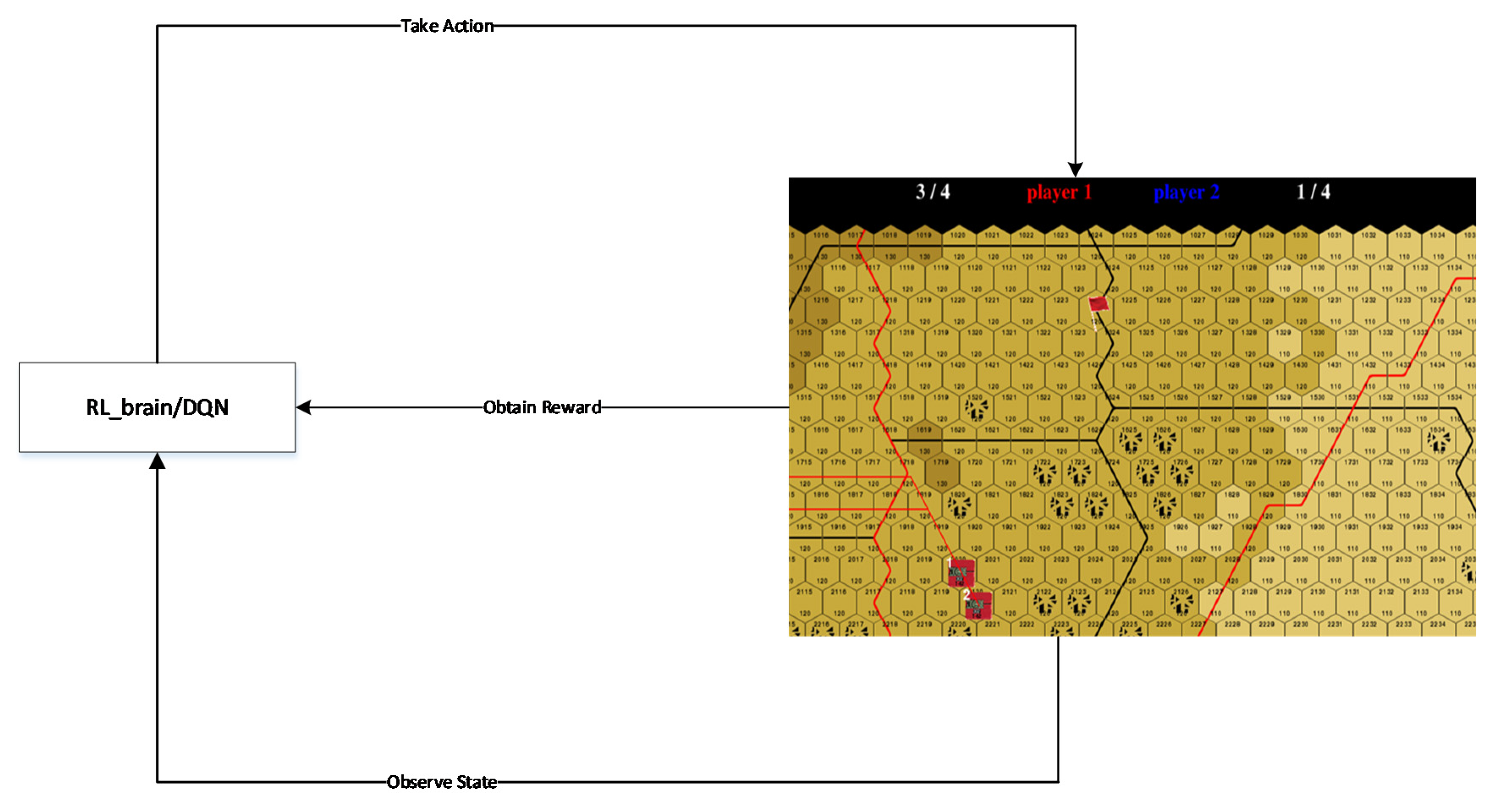
In this paper, we utilize the DQN algorithm to implement the operator’s action selection, which is to set an RL_Brain to select actions. RL_Brain is a brain that deduces relative to the entire smart warfare game. It is set up as a two-layer network, with 10 neurons in one layer and the ability to output actions. The action selection of the red side obtains the XY coordinates of the rank of the red side, which is then passed into the observation as an observation input array. XY coordinates are the coordinates of each hexagonal grid in the wargame environment. Each hexagon has an XY coordinate. This coordinate can determine the position of the other party when shooting, and also determine the destination of our party. The RL_Brain-trained neural network selects the maximum Q-value action, decides the output state action space value, calls the corresponding movement function or shooting function after determining the value, and then determines the next action, as shown in Figure 4.

3. Construction of Intelligent Wargame Model Based on Prior Knowledge-Deep Q Network (PK-DQN) Algorithm

How to effectively make, evaluate and choose the action plan is a challenging problem that restricts the intelligent decision system to enter the practical application. To solve this problem by traditional methods, it is necessary to model the environment and rules reasonably. However, in many aspects of modeling, human subjective factors are inevitably introduced, which greatly reduces the accuracy and rationality of the final decision-making scheme. Therefore, we break through the traditional method of action plan reasoning based on model knowledge, and explore the technical solution combining the experience judgment and intuitive reasoning that fit the decision-making thinking of commanders.
As one of the methods to solve sequential decision making, reinforcement learning (RL) has been predominantly combined with deep learning in the field of artificial intelligence in recent years, which has achieved remarkable results and become a representative machine-learning method to break through cognitive intelligence. These mechanisms and methods of reinforcement learning can be used as the key technology of simulation, deduction and evaluation of the scheme, because they accord with the decision-making thinking mode of commanders for complex combat problems.
This paper introduces the DQN algorithm in reinforcement learning for intelligent Red and Blue Armies in military chess deduction. Red AI is built with the DQN algorithm, Blue AI is built with rules. A Red operator based on DQN algorithm is trained with rules-based blue algorithm through a red-blue game, which provides more realistic simulation scenarios and solves battle tactics. The practical problem of a low AI level in military wargame deduction assists command and decision makers in accurately understanding, rational thinking and quick decision-making of battlefield situations. Based on the analysis of state space and the action space of wargame deduction, the feasibility study is carried out by using the DQN algorithm of reinforcement learning. The state space of wargame deduction can be defined as position coordinates X and Y, and the real-time state (maneuver, concealment, design) of operators can form the state space of chess deduction. The action space of chess deduction can also be defined as specific and limited operation. Therefore, this section first describes the design of a smart chess system, then presents the expert knowledge model in the field of dispatching chess, and builds the action strategy model based on the DQN algorithm, and finally establishes the process model of integrating prior knowledge with the DQN algorithm i.e., the PK-DQN algorithm.

3.1. Design of Intelligent Wargame System

The red square operator of the whole intelligent wargame system inputs the state of a certain moment (maneuver, concealment, shoot) as well as the XY coordinate, while the terrain reads the excel table within the scope of battle, and the terrain hexagon lattice mainly includes the high level and label. The whole deduction environment is based on this system setting.
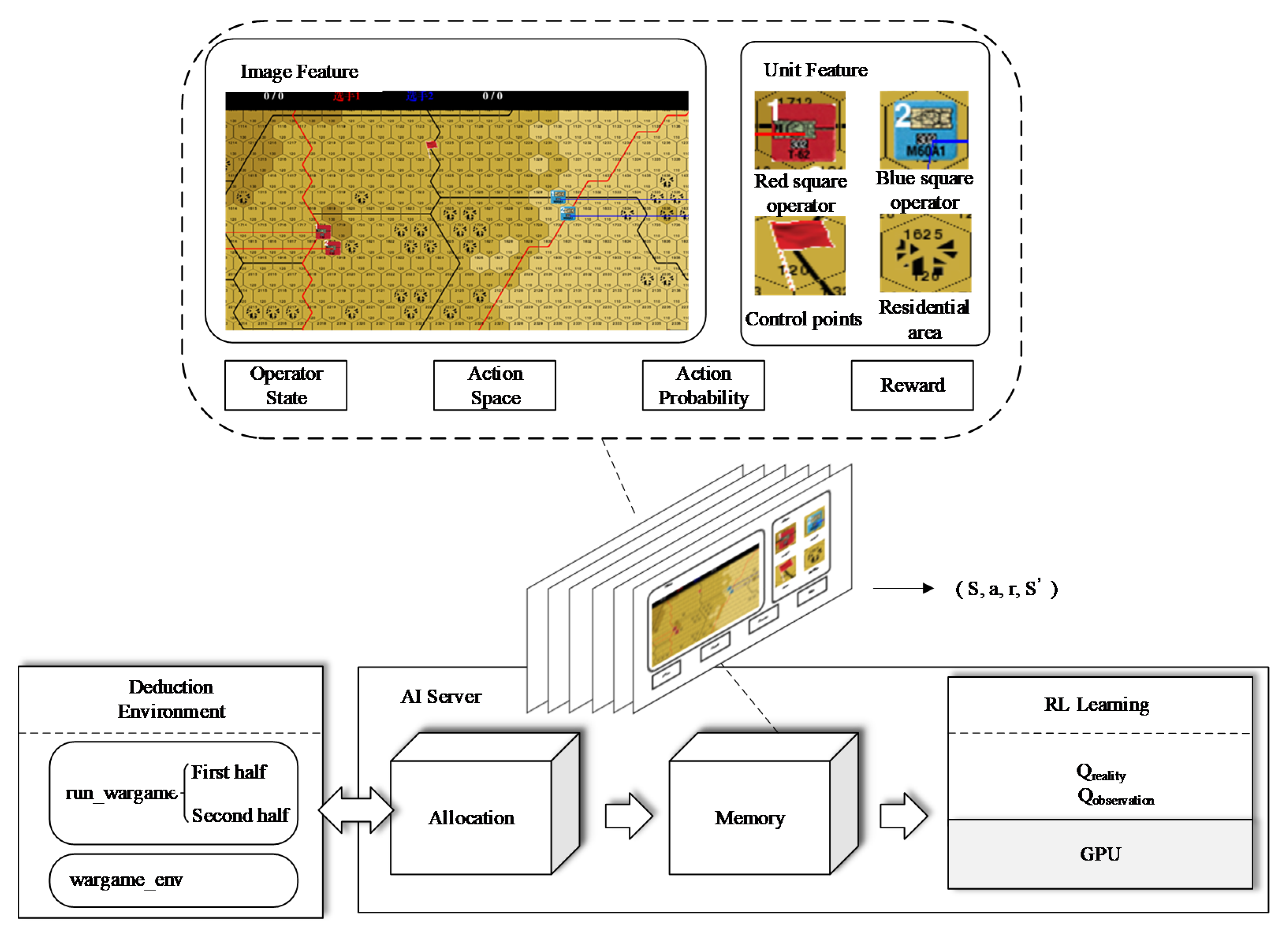
The whole game environment is mainly composed of four modules, including learning module, deduction environment module, distribution module and storage memory module. The relationships among the modules are shown in the following Figure 5:
RL Learning module: the learning module is the core part of intelligent algorithm. By calling status, action, return value and next step status in batch size, neural network parameters are constantly updated. In order to reduce the cost function value efficiently, the learning module and memory module use a storage structure together. The trained model synchronizes to the deduction environment module in the form of point-to-point quickly, and then realizes the selection of the model of the action.
Deduction environment module: The deduction environment module consists of the interaction between the deduction environment and AI model, as well as the basic functions of defining the whole deduction environment. The functions comprise judging the winning conditions, checking the number of rounds, reading in the deduction scenario, etc. It saves the basic parameters related to the deduction, including both sides’ scores, both sides’ kill numbers, both sides’ survival numbers and both sides’ win numbers. The whole environment generates a confrontation environment of red side and blue side, and sets a clear number of rounds, which enables playing a game within the number of rounds.
Allocation module: the allocation module is responsible for collecting the sample data obtained from each step from the deduction environment module, including the current status, return value, action and next step status, and passes the collected data into the storage memory module in the form of an array.
Memory module: memory module is a part of memory space, which is used to set the size of memory space, and it then transfers the allocated array data and stores them in turn. When the storage space is larger than the memory space, the prior data are removed, and the data of batch size are also extracted to the learning module to update the strategic network, so as to reduce the loss function.

3.2. Prior Knowledge of Intelligent Wargame

In the training process of intelligent wargame, it is found that only relying on DQN algorithm for training, there is a large randomness of the results after each game starts, and the overall convergence speed is slow. Therefore, this paper considers introducing the concept of prior knowledge. By adding prior knowledge to the action selection process, it can prevent the algorithm from falling into local optimum, reduce invalid exploration and improve the learning efficiency of the algorithm. The a priori knowledge considered in this paper is divided into two parts. The first part is the basic function realization of intelligent wargame, including the basic definition of wargame action. Another part is the prior knowledge based on the experience of domain experts, which can accelerate the convergence of the training process.

3.2.1. Prior Knowledge of Basic Functions of Wargame

The design of an intelligent wargame must be based on the corresponding basic functions. By invoking basic functions, the algorithm of intelligent wargame can be realized, and finally the establishment of intelligent engine can be realized. Its main functions are as follows:
(1)
Move function
Initialize the starting position, assign the value in the scenario, calculate the X, Y coordinates of each operator, obtain the coordinates of the surrounding hexagonal lattice, select a coordinate to assign the value in the acquired hexagonal lattice coordinates, and then move the coordinates, including the East, West, Northeast, Northwest, Southeast, Southwest six directions.
(2)
Integral function of shooting reward
Shoot the enemy operator, obtain the coordinates of the enemy operator, and then judge whether the enemy operator exists after shooting. If it exists and the coordinates correspond to the coordinates of the enemy operator, the corresponding reward score will be obtained, otherwise no score will be obtained.
(3)
Shooting function
Obtain the coordinate position of the operator, judge whether the enemy operator can be observed by calling the visual function, if the observed distance can be shot, set the strike effect according to the enemy and distance.
(4)
Obtain adjacent coordinate function
Input the X and Y coordinate of the operator to represent the coordinates of the hexagonal lattice, and output the list to represent the coordinates of the surrounding hexagonal lattice in the form of a list.
(5)
Query the distance between two hexagonal lattices
Input X0, Y0, X1, Y1 as the coordinates of int, indicating the coordinates of the hexagon lattice at the beginning and the hexagon lattice at the end, and output as the distance between the two hexagon lattice.
(6)
Obtain operator state information function
The current coordinates of the operator and the maneuvering state of the turn are obtained by the function.
(7)
Check whether the operator can observe the opposite operator
Input the state information of the opposite operator, observe that the output of the opposite operator is true, but not false.
The rule of the whole intelligent wargame is that red and blue fight each other, and the operators of both sides can move, hide, direct aim and indirect aim. In this way, ‘mobile’ means to input X and Y coordinates, which represent the coordinates of adjacent hexagons, output effect, and move the operators. ‘Hide’ means to ensure that the operators enter the concealed state, which is not conducive to being attacked. The direct aim is to input enemy operators, the output phase should be the shoot effect, the shoot enemy operator; input X, Y represent target hexagonal grid coordinates, output effect, and indirect aim target hexagonal grid.

3.2.2. Prior Knowledge of Domain Experts

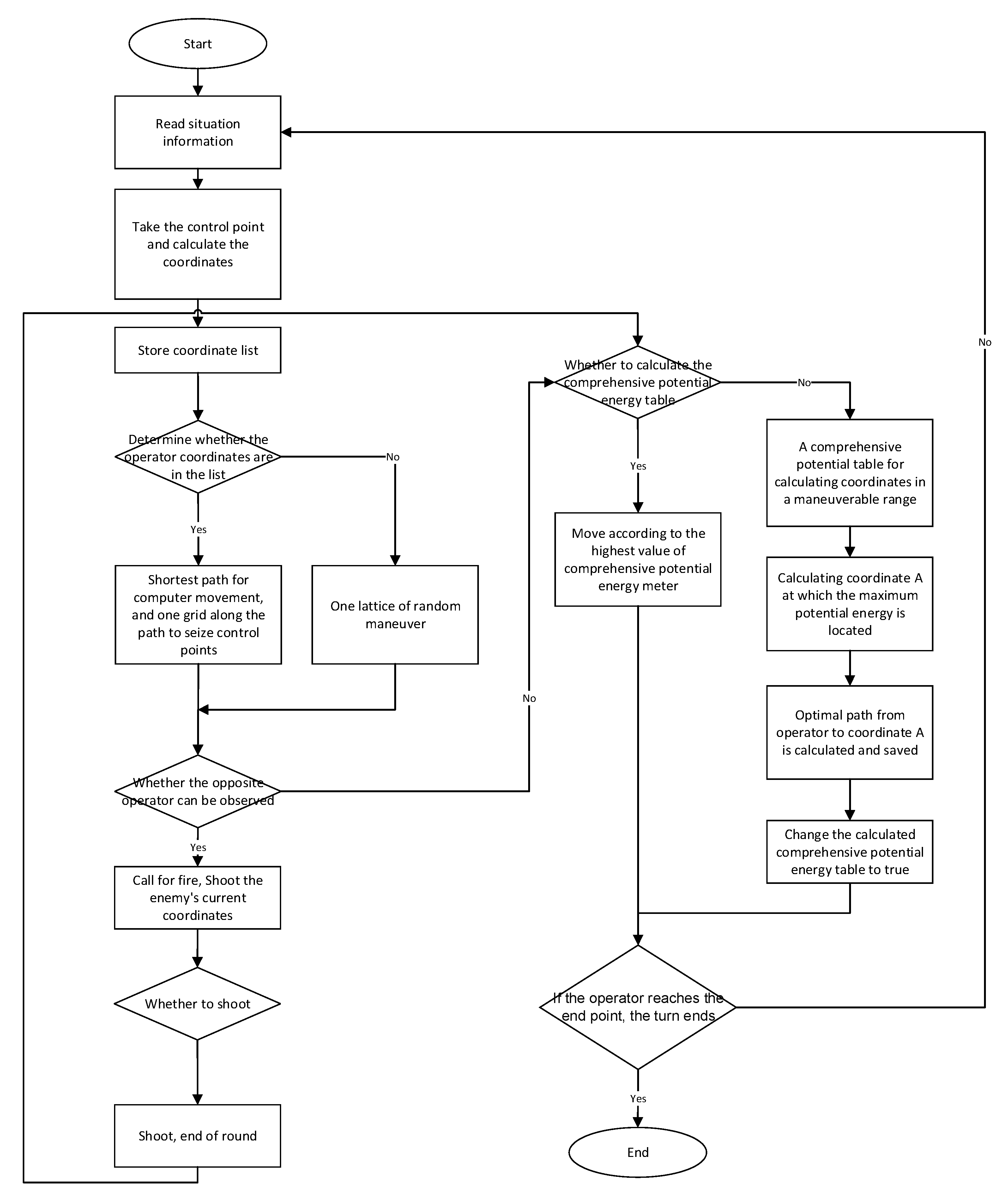
This paper designs the prior knowledge of the experts in the field of intelligent wargames, which mainly include the moving strategy and shooting strategy of the intelligent wargame operators. At the same time, this paper also constructs the sub-strategy of the professional players in the process of the competition based on the data of the wargame competition, forms a static comprehensive potential energy table, and realizes the prior knowledge of the experts in the field through a full simulation, combining the prior knowledge of the experts in the field with DQN calculation. The method achieves accelerated convergence of loss function. The designed operator action strategy based on prior knowledge of domain experts is shown in Figure 6:
Firstly, read the location, terrain and contention point information of both sides. Then, taking the point of contention as the center, the coordinates around the point that can maneuver to the control point in a round are calculated, and the coordinate list is stored. Determine whether the current coordinates of the operator are in this list. If so, the shortest path of the computer movement, the soldier moves 1 grid along the path to the point of contention. Judge whether the opponent’s algorithm can be observed, and if so, prepare for long-range shooting. Then judge whether it meets the shooting conditions. If so, it will strike the enemy’s current coordinates. If not, judge whether the comprehensive potential energy table has been calculated. If not, according to the maneuverable range and the comprehensive potential energy of the coordinates within the moving range of the computer, move to the maximum potential energy coordinate. If the potential energy is in the same direction, the killing potential energy is compared, and then the maneuver path from the current coordinate to the coordinate a is generated, which is called repeatedly. Finally, the turn ends when it reaches the end of the path sequence and moves to the next coordinate of the path sequence.

3.3. Action Strategy Based on DQN Algorithm

3.3.1. Policy Space Description

In order to realize the intelligent wargame based on DQN algorithm, the description of the operator’s state space and action space should be made clear. The state space mainly includes the X and Y position coordinates of the deduction scenario, and the number of values is 30 × 30. The action parameters of the operator mainly include maneuver, shooting and concealment, as shown in Table 1.
Among them, the maneuverable directions of the operator are 7 states of East, West, Northeast, Northwest, Southeast, Southwest and Static, which are defined as 0~6 respectively, as shown in Table 2. The firing states of the operator in one cell are shooting, not shooting and concealing.

3.3.2. Reward Function Design

The reward function is mainly divided into distance reward and shooting reward. Distance reward is used to obtain R1 reward values for the winning control point. The European distance between the route selection operator and the winning control point is set as the greater the European distance from the winning control point, the lower the reward value. If the winning control point is obtained, the return value is set as a larger value. Finally, the observation values x, y coordinates, actions and return values of each step are stored in the transition for later recall study.
reward = reward − distance2
If the shooting reward is to shoot and hit the enemy operator, R1 rewards will be given, otherwise no reward value will be given.

3.3.3. Path Planning

According to path planning set by reward, the shortest distance from the control point will be automatically found. In the early stage of training, the path selection will appear in the repeated movement of a point, but in the late stage of training, we will see the red square operator and gradually find the closest distance to the control point. As shown in the figure below, the red line behind the red square operator is the trajectory of the operator’s movement. The operator has learned that the best way to reach a hold point.

3.3.4. Shooting

In this paper, the reward value is to define the effect of shooting. Due to the large shooting space, the training convergence will be too slow. Therefore, for the shooting part, the shooting rules are integrated to speed up the convergence of the training. The shooting rules mainly include two ideas: whether it can be intervisibility, and if it can be intervisibility, direct shooting. Another idea is to judge the distance between all operators of both sides and calculate the nearest distance between them. According to the actual combat operation of professional players, when the distance between operators is 12, the shooting effect is the best. Therefore, 12 is taken as the mark point. If the distance is greater than 12, the operator moves towards the point of contention continuously. If the distance between operators of both sides is less than or equal to 12, an enemy operator remains still. The state can be used for shooting, otherwise the operator moves to the nearest distance of the control point and fire.

3.4. DQN Algorithm Model Combined with Prior Knowledge

This paper defines prior knowledge as follows:
(1)
Let the state sequence of DQN algorithm be S , s i represents the state of different stages and its formula be:
S = [ s 1 , s 2 , s 3 , , s i ] , i = 1 , 2 , 3
(2)
Let the action sequence as A , a i represents actions performed at different stages and its formula is:
A = [ a 1 , a 2 , a 3 , , a i ] , i = 1 , 2 , 3
(3)
Let the characteristic state sequence of prior knowledge strategy be P , p i represents the characteristic states of different stages and its formula be:
P = [ p 1 , p 2 , p 3 , , p i ] , i = 1 , 2 , 3
When the characteristic state p i appears, the optimal action selection is a * , then the state is set as the characteristic state p * . The mapping relation p * a * between the characteristic state and the optimal action is established. The rules formed by this mapping relationship are called prior knowledge. Among them, the state sequence S is the input of the algorithm, the characteristic state P may be the input of the algorithm or other signals, and the characteristic state and the state sequence satisfy P S = .
(4)
According to the concept of Q value in DQN algorithm, the prior Q value vector is defined as Q p , and the Q p formula is:
Q p = ( Q p a 1 , Q p a 1 , Q p a 1 , , Q p a i ) T
where Q p a i is the prior Q value of action a i , 0 < Q p a i < 1 , and vector Q p is the set of prior Q values of all actions when the prior knowledge is known.
(5)
Because there are many factors that affect the result of decision-making, and prior knowledge has only partial influence on the decision-making of action selection, therefore, the influence of prior knowledge on action selection is not completely determined. According to the influence degree of prior knowledge on action selection, this paper sets μ as the influence degree of prior knowledge on action selection. When the feature state p * appears and the prior knowledge is completely related to the selection action a * , μ = 1 . 0 < μ 1 , there is no prior knowledge that has no effect on action selection.
(6)
According to the above definition, after the prior knowledge is added, the final action selection Q value is Q F . First normalize Q , then calculate Q F , and the Q F calculation formula is:
Q F = μ Q p + ( 1 μ ) Q
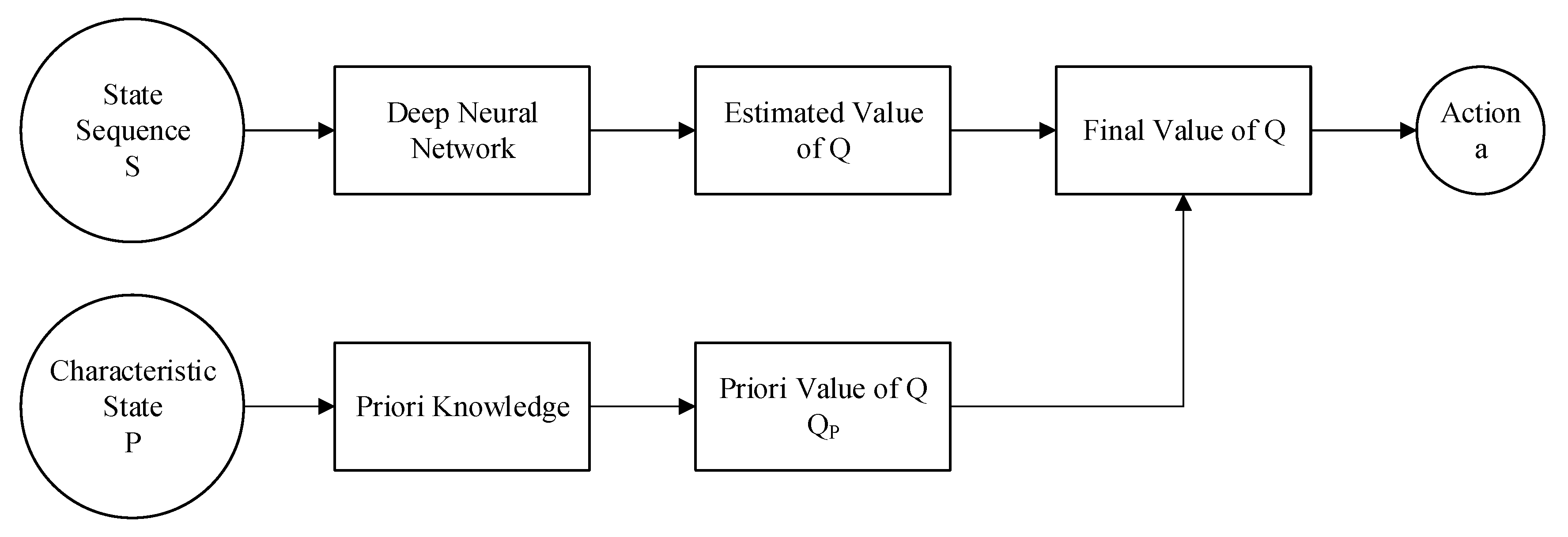
where Q is the Q value vector selected by DQN algorithm according to the action estimated by the current state. When the characteristic state p * appears, the Q F value of each action is calculated according to Formula (7), and the action is directly selected according to the maximum Q F value; when the characteristic state p i does not appear, the Q value of the action is estimated according to the DQN algorithm, and then the action is selected according to the ε g r e e d y rule. There are three main advantages: firstly, by introducing prior knowledge, when the feature state p * is detected, it can affect the action selection process according to the prior knowledge p * a * , reducing unnecessary exploration; second, the introduction of prior knowledge does not affect the training process of the algorithm; finally, when there is no feature state, it can judge the action selection through the algorithm to fully explore the state space. The introduction process of prior knowledge is shown in Figure 7.
By introducing prior knowledge and intervening in the action selection process of the DQN algorithm, valuable information can be fully used during algorithm training. Prior knowledge such as domain expert knowledge, feature signal and classification feature can be added to algorithm training, so that the improved model can effectively avoid invalid exploration. The improved algorithm improves the convergence speed and accuracy of the algorithm, which can effectively improve the training efficiency and save the training cost. During the training process, the PK-DQN algorithm selects actions and controls the selection process according to whether there is characteristic state. According to the definition of a priori knowledge, a priori Q value and μ in the above formula, the a priori knowledge is introduced into the DQN algorithm to build the PK-DQN algorithm, and the PK-DQN algorithm is shown in Figure 8.
Algorithm: Prior Knowledge-Deep Q Network (PK-DQN) is combined with prior knowledge. Input: state s, output: Q neural network weight.
  • Step 1: Initialize experience value D with capacity N
  • Step 2: Initialize Q neural network and set the random weight as θ ;
  • Step 3: At the beginning of iteration t = 1, input the initial state s t ;
  • Step 4: If the characteristic state p * appears, calculate the Q F value from the formula, and select the action a * with the largest Q F value to output; otherwise, output the action a t according to the ε g r e e d y rule;
  • Step 5: Executes action a * or a t ;
  • Step 6: Obtains the feedback r t value and s t + 1 ;
  • Step 7: Store ( s t , a t , r t , s t + 1 ) in the experience pool;
  • Step 8: Judge whether the data amount in the experience pool reaches n. if it reaches n, train Q neural network, and update the weight θ of target Q neural network after constant C time steps; if it does not reach n, repeat steps 3–8. When the value θ is less than the threshold value, the algorithm is considered to reach the convergence state.
The above figure is the detailed flow chart of the algorithm, in which the dotted line part indicates the introduction of prior knowledge into DQN algorithm. This is the comparison between the workflow of PK-DQN and DQN. The part of PK-DQN which introduces prior knowledge is not found in the original DQN algorithm. The improvement of this work will significantly improve the effect of the whole method. Next, through specific experiments to verify the improvement effect of the PK-DQN algorithm.

4. Experimental Verification

In this paper, the training environment is based on the intelligent game simulation environment independently designed and developed by our team. The PK-DQN algorithm and DQN algorithm control operators are used to fight each other, including autonomous arrival at the point of contention and shooting each other. The stability and convergence rate of the two algorithms are compared to verify the influence of the introduction of prior knowledge on the training effect of the algorithm.

4.1. Experimental Platform

In order to verify the effectiveness of the PK-DQN algorithm, this paper uses the self-developed simulation environment as a test example, and the main configuration of the experiment is listed as follows:
(1)
Win 10: operating system, various task processing.
(2)
CUDA v8.0: GPU C language library. Calculate the same device architecture.
(3)
cuDNN (v6.0.21): deep learning primitive library based on CUDA.
(4)
Tensorflow (v1.0): a deep learning framework developed by Google.
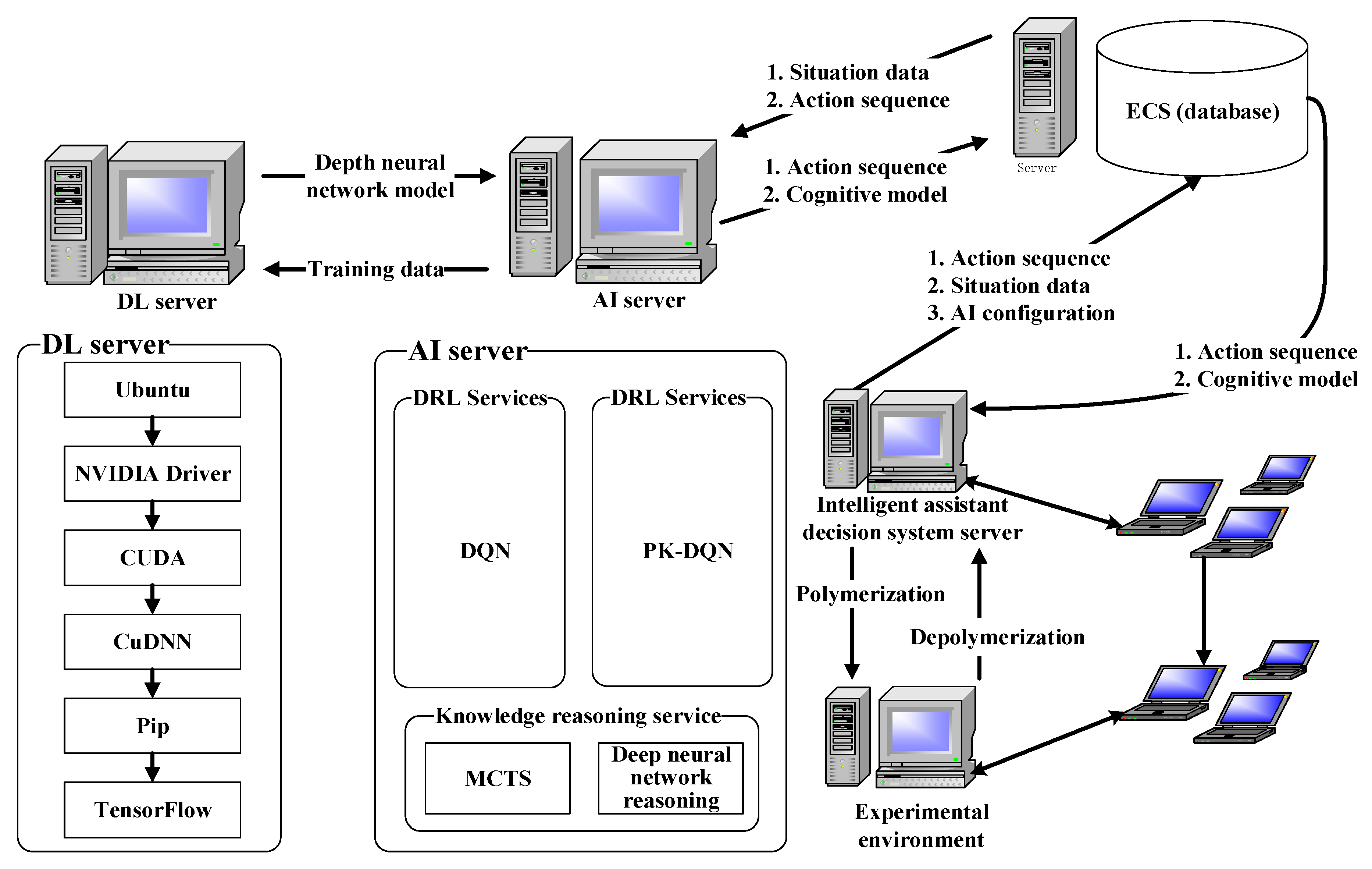
The whole environment includes the DL (Deep Learning) server and AI server. The AI server is configured with the DQN algorithm and PK-DQN algorithm for data training, which is transmitted to the DL server after training to form a deep neural network model. The cloud server transmits the original confrontation data and action sequence to the AI server, and receives the action sequence and cognitive model processed by the AI server. The cognitive model and action sequence formed are further transmitted to the intelligent decision-making system, and then to the experimental environment for simulation and deduction through decoupling. The experimental environment obtains new data through deduction, which is aggregated and then transmitted to the intelligent decision-making system. The intelligent decision-making system retransmits the new data, AI configuration and action sequence to the cloud server for a new round of training, as shown in Figure 9.
Scenario Description:
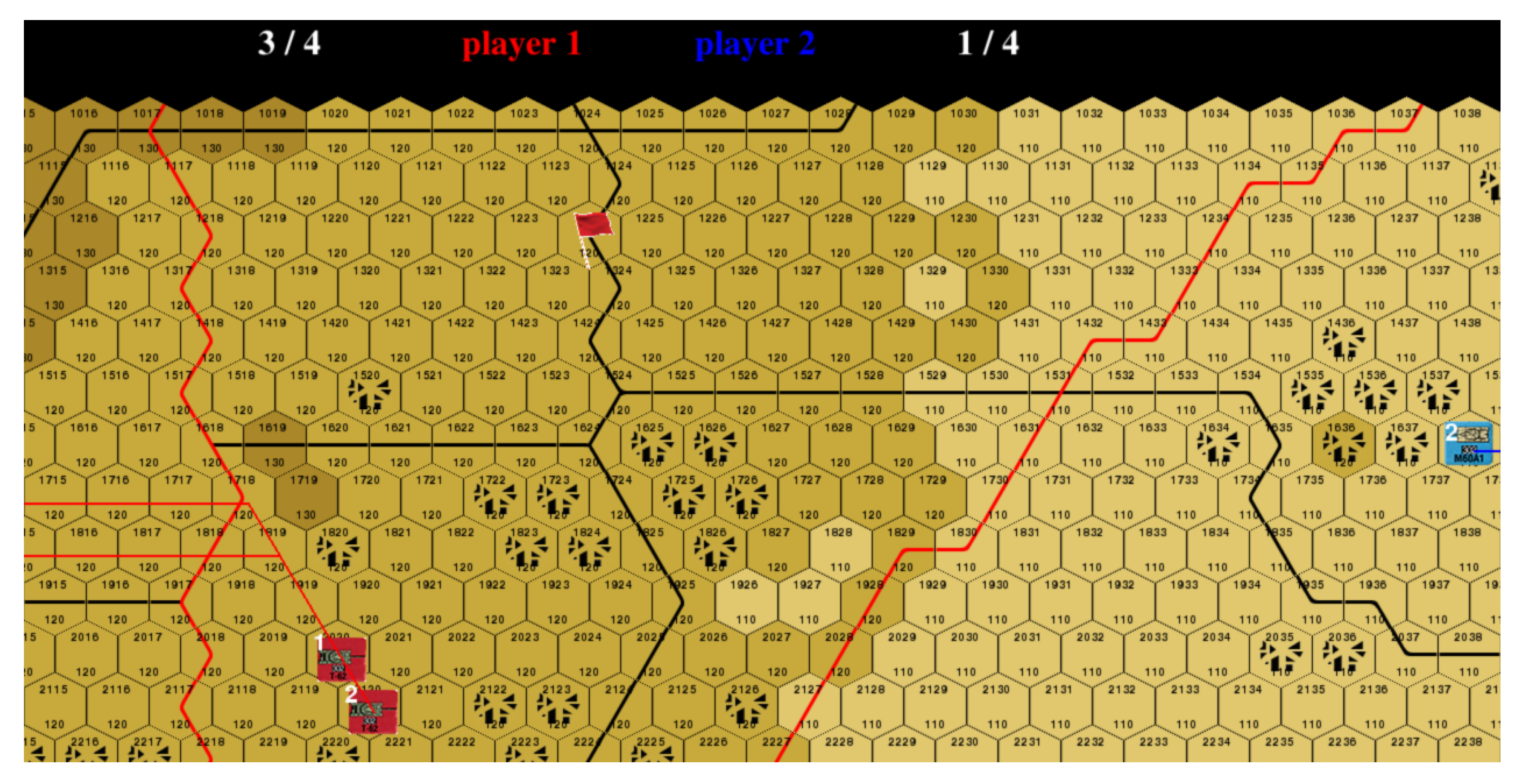
In this experiment, two operators, red and blue, are supposed to fight in the environment. The winning condition is to seize the red flag to seize the control point or to destroy all the operators of the enemy. At present, the urban residential area map is used, and the terrain of the main battlefield area is shown in the Figure 10 below.
The details are as follows:
(1)
Elevation: elevation information is represented by color depth. There are five different colors to represent five different elevations. Elevation gradually increases with color from light to depth, and the height difference between adjacent changing colors is 20 m.
(2)
Operators: two for red and two for blue, each of which represents platoon, the minimum resolution unit of the army armored synthetic battalion. The attributes describing the operators mainly include two categories: tactical command decision state space and tactical action space.
Consumption: since the movement of the operator will consume oil, the initial oil quantity is set in the environment. The oil quantity will be consumed every time the operator moves a grid; the oil consumption varies with different elevations, and the higher the elevation, the greater the oil consumption.
(3)
The map size is 66 × 51 and the map number is 83.
(4)
There is a total of 1 control point, which are: control point, coordinate 80,048, score 80.
(5)
There are two pieces in the red and blue sides respectively. The initial position and terrain of the two tanks are described as follows Table 3:

4.2. Experimental Results and Analysis

In this experiment, PK-DQN algorithm is applied to the self-developed confrontation environment, and the performance of the algorithm is tested and compared with the DQN algorithm. Through the comparative analysis of the experimental results, the experimental results are shown in Figure 11. The horizontal axis in the figure represents every step of training. The vertical axis loss represents the size of the cost function L i ( θ i ) .
(1)
In terms of convergence speed, the DQN algorithm needs about 1500 steps to reach the convergence threshold of the algorithm, which is still not less than 1000, while the PK-DQN algorithm can reach the convergence threshold of the algorithm in 1500 steps. Compared with the DQN algorithm, the PK-DQN algorithm is faster and more stable. See Figure 11 for details. The reason is that by introducing prior knowledge, the PK-DQN algorithm reduces the number of times of exploration in the training process, speeds up the optimization speed of Q neural network, and the algorithm converges rapidly with little fluctuation, so it can reduce the intervention of prior knowledge in the action selection process after the algorithm converges, and at the same time ensure the training efficiency and stability of the algorithm.
(2)
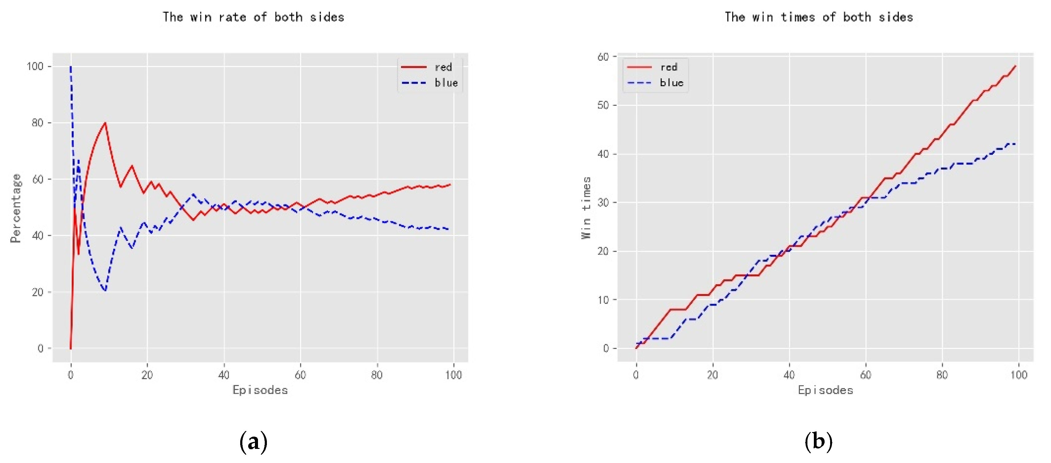
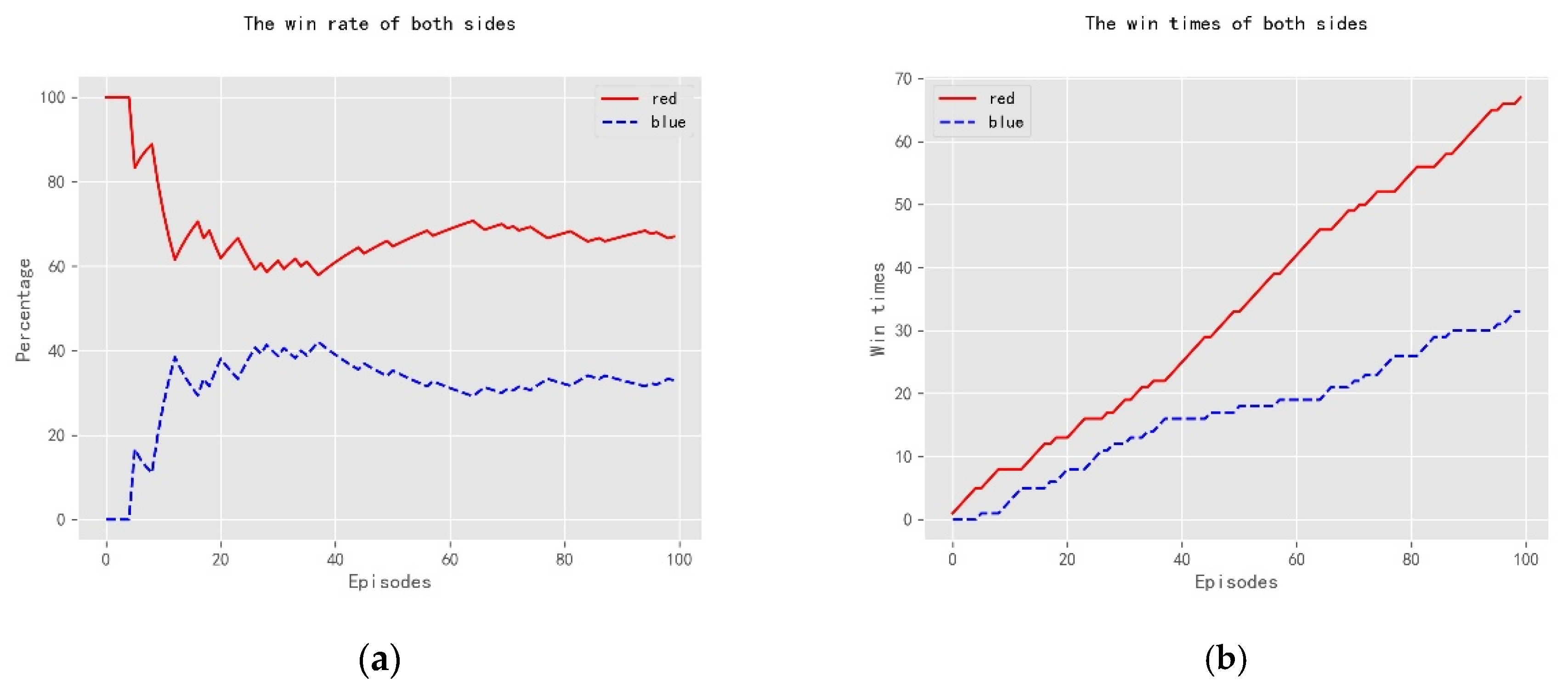
In the aspect of algorithm winning rate, to verify the faster convergence of PK-DQN, we guarantee that PK-DQN and DQN will be trained together for 24 h at the same time, then PK-DQN and DQN will be used as red AI and rule-based Blue AI to compete against each other, and then observe the winning rate of the two algorithms compared with rule-based Blue AI. The winning rate of the DQN algorithm and the PK-DQN algorithm is 57% and 67% respectively, as shown in Figure 12 and Figure 13. It shows that the introduction of prior knowledge can obviously improve the intelligence of operators. The specific winning games are shown in the Table 4 and Table 5 below.
(3)
In terms of algorithm efficiency: to verify the efficiency of training, we use the 80% winning rate as the verification standard to see how long it takes for PK-DQN and DQN to reach 80% winning rate. Both algorithms are against the rule-based blue AI. It takes 23 h and 17 min for PK-DQN to be stable to win rule-based AI in the confrontation, and 32 h and 39 min for the DQN algorithm alone. This further shows that the introduction of prior knowledge can significantly accelerate the convergence speed of the algorithm. The experimental results are shown in Table 6, where T is the total training time and N is the number of operators (tanks) in the antagonism.
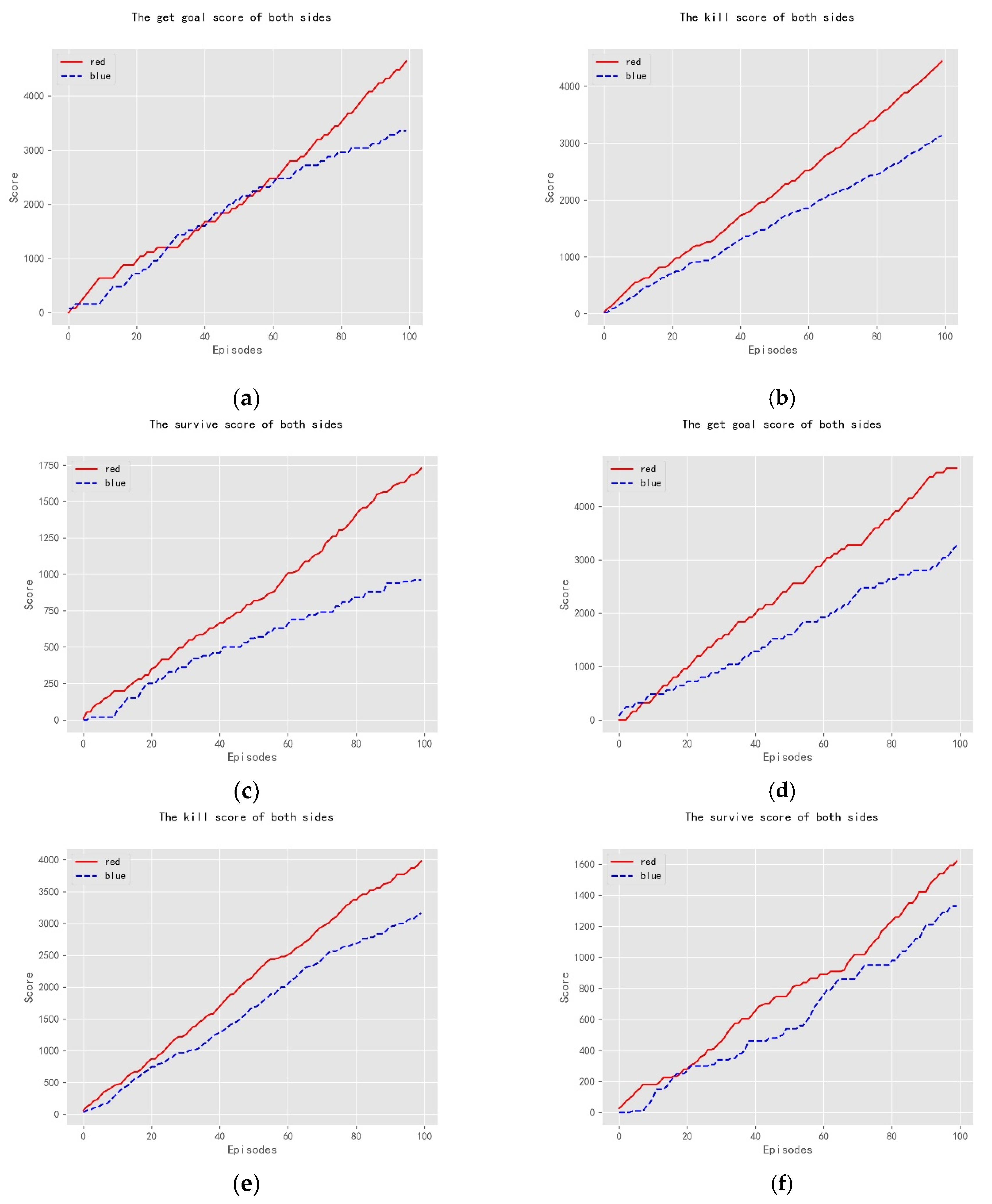
The experimental results show that the PK-DQN model can reduce the number of times to explore during training, and improve the problem that the DQN algorithm takes too long to train. It shows that the introduction of prior knowledge improves the performance of the DQN algorithm, and has a certain theoretical significance for improving the efficiency of the algorithm, the detail score is shown in Figure 14.

5. Conclusions

The main innovative work of this paper is to independently develop an intelligent wargame deduction environment, which has been verified by experiments and configured with a series of basic functional interfaces to achieve the confrontation of different types of operators on different maps. It can provide validation and effect analysis for subsequent large-scale and different kinds of wargame combat deduction experiments. We first used the Q-learning algorithm to design the game algorithm. Q is Q (s, a), s is the state and a is the action. The main idea of the Q-learning algorithm is to construct a Q-table to store static and action into a Q-table, and then select the action that can obtain the maximum benefit according to the Q value. However, we find that it is problematic to use Q learning alone. Q-tables are limited. If the state space and action space are very large, it is difficult for us to store them all. Therefore, we introduce the DQN algorithm. We use function approximation to solve the problem of too large state space, complex action space and insufficient computer memory. By expressing Q (s, a) with a function instead of a Q table, the function can be linear or non-linear. At the same time, this paper uses this platform to verify that the DQN algorithm can be applied in the field of wargames, to achieve the deduction of intelligent wargames, and to explicitly verify that the DQN algorithm can defeat high-level rule-based opponents, which provides the first step of work verification for the exploration of the field of intelligent wargames and the deduction of intelligent games. At the same time, it is found that DQN training is difficult to converge for a long time during the training process, so a priori knowledge is introduced to improve the DQN algorithm, and a PK-DQN algorithm is proposed. The experimental results show that the PK-DQN model can reduce the number of times it is required to explore during training, and improve the problem that the DQN algorithm takes too long to train. This shows that the introduction of prior knowledge improves the performance of the DQN algorithm, and has a certain theoretical significance for improving the efficiency of the algorithm. Subsequently, work will be undertaken on this platform, including the experimental validation of the DDQN algorithm, A3C, PPO algorithm and a series of improved algorithms in the deductive antagonism of intelligent wargame, as well as the study of collaboration between multi-agents.

6. Patents

The experimental platform used in this paper has declared the copyright of computer software. (grant number 2020R11S0628066).

Author Contributions

Project administration, B.T.; Supervision, X.Z. and B.Y.; Writing—original draft, Y.S.; Writing—review and editing, W.Z. and T.Z. All authors have read and agreed to the published version of the manuscript.

Funding

This work was supported in part by the Innovation and Creativity Research Program for Doctoral Students of Nanjing University (grant number CXCY19-19). This work was also supported by the CSC scholarship. This work was supported by National Nature Science Foundation under Grant 61876079.

Conflicts of Interest

The authors declare no conflict of interest.

Appendix A

Explanation of Terminologies
Wargame: a combination of ‘game’, history and science. The simplest way is to think of wargame as chess, but there are more complex ways to move the pieces and capture your opponents.
Operator: Each operator represents units in Chess of War, and in this paper mainly refers to tanks.
Point of contention: a hexagonal coordinate that means occupying a favorable terrain or a place of strategic value.
Scenario: a specific antagonistic environment in chess deduction, including specific terrain and operators and tasks to be performed.
The comprehensive potential energy: this is a comprehensive judgment of the quality of a hexagonal lattice. The comprehensive potential energy is related to the snatch potential energy, the kill potential energy and the offline potential energy. It is necessary to calculate the three potential energies of all coordinates in the maneuverable range, multiply them by the weight of the corresponding potential energy, respectively, and then sum them. Snatch potential energy is a measure of the possibility that a tank can reach a critical point when it is in the hexagonal lattice; kill potential energy is a measure of the advantages and disadvantages of the hexagonal lattice in killing the enemy; off-line potential energy is to analyze the previous deduction data and extract the advantages and disadvantages of each hexagon to measure.
The comprehensive potential energy of each coordinate is equal to the three potential energies of the coordinate multiplied by their respective coefficients, and then the sum is calculated.
Comprehensive potential energy = snatch potential energy * snatch potential energy coefficient a + kill potential energy * kill potential energy coefficient B + offline potential energy * offline potential energy coefficient C.

Appendix B

Detailed Explanation of DQN Algorithm
Line 1, the playback memory D is initialized, and the number of data pieces it can hold is N
Line 2, the random weight θ is used to initialize the action value function Q
Line 3, initialize θ = θ to calculate the action behavior value Q of T D target
Line 4, loop each event
Line 5, the first state s 1 of the event is initialized, and the feature input corresponding to the state is obtained by preprocessing
Line 6, loops through each step of each event
Line 7, use probability ε to select a random action a t
Line 8, if the small probability event does not occur, the greedy strategy is used to select the action a t = arg max a Q ( ϕ ( s t ) , a ; θ ) with the largest current value function. Note that the value function network used in selecting the maximum action and the network used for approximating value function are the same network, corresponding to θ .
Line 9, perform action a t in the simulator, observe the return r t , and image x t + 1
Line 10, set s t + 1 = s t , a t , x t + 1 , preprocess ϕ t + 1 = ϕ ( s t + 1 )
Line 11, store conversion ( ϕ t , a t , r t , ϕ t + 1 ) in playback memory D
Line 12, a conversion sample data is randomly sampled from the playback memory D and represented by ( ϕ j , a j , r j , ϕ j + 1 ) .
Line 13, judge whether it is the termination state of an event. If it is, the T D target is r j . otherwise, the T D target r + γ max a Q ( s , a ; θ ) is calculated by using T D target network θ .
Line 14, perform a gradient descent algorithm
Δ θ = α [ r + γ max Q ( s , a ; θ ) Q ( s , a ; θ ) a ] Q ( s , a ; θ )
Line 15 updates the network parameters approximated by the action value function θ = θ + Δ θ
Line 16, the T D target network weight is updated every C step, that is, θ = θ
Line 17, end the loop for each event
Line 18, end the loop between events

Appendix C

Main Rules of the Game
Maneuver: the intelligent algorithm sends maneuver or stop command to the operator (tank) and specifies the maneuver route for the operator. The system automatically converts the operator’s maneuver path into hexagonal lattice maneuver path according to the maneuver route specified by the deduction personnel.
Observation: the system updates the situation every 1 s, updates the position of operators (tanks) of both sides according to the situation, automatically makes observation judgment and displays the results.
Engagement: if the target is observable and within the range of the weapon, the operator (tank) can fire at long range.
Win or lose: a game is judged by the net score. The net score is calculated as the difference between one party’s “seizing the critical point + the score of its own surplus force + the score of annihilating the opponent’s force” and that of the other party’s “seizing the critical point + the score of its remaining force + the score of annihilating the opponent’s force” is the net score. If the net score is positive, the game will win. If the net score of both sides is 0, it will be a draw.

References

  1. De Loura, M.A. (Ed.) Game Programming Gems 2; Cengage Learning: Boston, MA, USA, 2001. [Google Scholar]
  2. Silver, D.; Huang, A.; Maddison, C.J.; Guez, A.; Sifre, L.; Van Den Driessche, G.; Schrittwieser, J.; Antonoglou, I.; Panneershelvam, V.; Lanctot, M.; et al. Mastering the game of go with deep neural networks and tree search. Nature 2016, 529, 484–489. [Google Scholar] [CrossRef] [PubMed]
  3. Nascimento Silva, V.; Chaimowicz, L. On the development of intelligent agents for moba games. In Proceedings of the 2015 14th Brazilian Symposium on Computer Games and Digital Entertainment (SBGames), Piaui, Brazil, 11–13 November 2015; pp. 142–151. [Google Scholar]
  4. Synnaeve, G.; Bessiere, P. A bayesian model for rts units control applied to starcraft. In Proceedings of the 2011 IEEE Conference on Computational Intelligence and Games (CIG’11), Seoul, Korea, 31 August–3 September 2011; pp. 190–196. [Google Scholar]
  5. Tian, Y.; Gong, Q.; Shang, W.; Wu, Y.; Zitnick, C.L. Elf: An extensive, lightweight and flexible research platform for real-time strategy games. In Proceedings of the 31st Conference on Neural Information Processing Systems (NIPS 2017), Long Beach, CA, USA, 19 May 2017; pp. 2656–2666. [Google Scholar]
  6. Wender, S.; Watson, I. Applying reinforcement learning to small scale combat in the real-time strategy game starcraft: Broodwar. In Proceedings of the 2012 IEEE Conference on Computational Intelligence and Games (CIG), Granada, Spain, 11–14 September 2012; pp. 402–408. [Google Scholar]
  7. OpenAI. Openai Blog: Dota 2. 2018. Available online: https://blog.openai.com/dota-2/ (accessed on 17 April 2018).
  8. Othman, N.; Decraene, J.; Cai, W.; Hu, N.; Low, M.Y.H.; Gouaillard, A. Simulation-based optimization of StarCraft tactical AI through evolutionary computation. In Proceedings of the 2012 IEEE Conference on Computational Intelligence and Games (CIG); Institute of Electrical and Electronics Engineers (IEEE), Granada, Spain, 11–14 September 2012; pp. 394–401. [Google Scholar]
  9. Vinyals, O.; Ewalds, T.; Bartunov, S.; Georgiev, P.; Vezhnevets, A.S.; Yeo, M.; Makhzani, A.; Küttler, H.; Agapiou, J.; Schrittwieser, J.; et al. Starcraft ii: A new challenge for reinforcement learning. arXiv 2017, arXiv:1708.04782. [Google Scholar]
  10. Weber, B.G.; Mateas, M.; Jhala, A. A Particle Model for State Estimation in Real-Time Strategy Games. In Proceedings of the Seventh AAAI Conference on Artificial Intelligence and Interactive Digital Entertainment; AIIDE 2011, Stanford, CA, USA, 10–14 October 2011; pp. 103–108. [Google Scholar]
  11. Anschel, O.; Baram, N.; Shimkin, N. Averaged-dqn: Variance reduction and stabilization for deep reinforcement learning. In Proceedings of the International Conference on Machine Learning, Sydney, Australia, 6–11 August 2017; pp. 176–185. [Google Scholar]
  12. Wu, B. Hierarchical macro strategy model for moba game ai. In Proceedings of the AAAI Conference on Artificial Intelligence, Honolulu, HI, USA, 27 January–1 February 2019; Volume 33, pp. 1206–1213. [Google Scholar]
  13. Schulman, J.; Wolski, F.; Dhariwal, P.; Radford, A.; Klimov, O. Proximal policy optimization algorithms. arXiv 2017, arXiv:1707.06347. [Google Scholar]
  14. Vincent, J. Humans Grab Victory in First of Three Dota 2 Matches against Openai. 2018. Available online: https://www.theverge.com/2018/8/23/17772376/openaidota-2-pain-game-human-victory-ai (accessed on 23 August 2018).
  15. Simonite, T. Pro Gamers Fend Off Elon Musk-Backed ai Bots—For Now. 2018. Available online: https://www.wired.com/story/pro-gamers-fend-off-elonmusks-ai-bots/ (accessed on 23 August 2018).
  16. Tavares, A.R.; Azpurua, H.; Chaimowicz, L. Evolving Swarm Intelligence for Task Allocation in a Real Time Strategy Game. In Proceedings of the 2014 Brazilian Symposium on Computer Games and Digital Entertainment; Institute of Electrical and Electronics Engineers (IEEE), Porto Alegre, Brazil, 12–14 November 2014; pp. 99–108. [Google Scholar]
  17. Hagelbäck, J.; Johansson, S.J. The rise of potential fields in real time strategy bots. In Proceedings of the Fourth Artificial Intelligence and Interactive Digital Entertainment Conference, Ronneby, Sweden, 22–24 October 2008. [Google Scholar]
  18. Ontanón, S.; Buro, M. Adversarial hierarchical-task network planning for complex real-time games. In Proceedings of the Twenty-Fourth International Joint Conference on Artificial Intelligence, Buenos Aires, Argentina, 25–31 July 2015. [Google Scholar]
  19. Ballard, B.W. The *-minimax search procedure for trees containing chance nodes. Artif. Intell. 1983, 21, 327–350. [Google Scholar] [CrossRef]
  20. Bošanský, B.; Lisý, V.; Lanctot, M.; Čermák, J.; Winands, M.H. Algorithms for computing strategies in two-player simultaneous move games. Artif. Intell. 2016, 237, 1–40. [Google Scholar] [CrossRef] [Green Version]
  21. Waugh, K.; Morrill, D.; Bagnell, J.A.; Bowling, M. Solving games with functional regret estimation. arXiv 2014, arXiv:1411.7974. [Google Scholar]
  22. Brown, N.; Sandholm, T. Superhuman ai for multiplayer poker. Science 2019, 365, 885–890. [Google Scholar] [CrossRef] [PubMed]
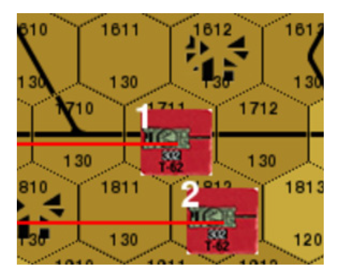
Figure 1. Schematic diagram of operator movement.
Electronics 09 01668 g001
Figure 2. Transformation of q-table.
Electronics 09 01668 g002
Figure 3. Algorithm framework of Deep Q Network (DQN).
Electronics 09 01668 g003
Figure 4. Action selection of intelligent wargame.
Electronics 09 01668 g004
Figure 5. Artificial intelligence (AI) Server implements how the AI model interacts with the environment. The Allocation Module is a station for sample collection, compression and transmission. The Memory is the data storage module, which provides training instances for the RL Learning. Note that these modules are decoupled and can be flexibly configured, so that our researchers can focus on the algorithm design and the logic of the environment. Such a system design is also applicable to other multi-agent competitive problems. The details of these modules are provided below.
Electronics 09 01668 g005
Figure 6. Flowchart of domain expert knowledge.
Electronics 09 01668 g006
Figure 7. Fusion process of prior knowledge and DQN algorithm.
Electronics 09 01668 g007
Figure 8. DQN algorithm model combined with prior knowledge.
Electronics 09 01668 g008
Figure 9. Based on the DL (Deep Learning) server, artificial intelligence (AI) server, simulation environment, intelligent assistant decision system and database environment, the architecture of the intelligent wargame system is constructed.
Electronics 09 01668 g009
Figure 10. Scenario description: red and blue have two operators (tanks) to fight each other. The red flag in the middle is the key point. The deeper the color is, the higher the elevation is. The grid of urban residential areas is indicated in black, which is conducive to concealment. The black line represents the first class road and the red line indicates the second class road. The operator (tank) has different moving speed on the first road and the second road respectively.
Electronics 09 01668 g010
Figure 11. (a) Performance of the DQN learning curve in simulation environment; (b) Performance of the PK-DQN learning curve in simulation environment. The X coordinate represents the number of training steps, that is, the total steps of confrontation training; the Y coordinate represents the size of the cost curve value L i ( θ i ) .
Electronics 09 01668 g011
Figure 12. (a) Win rate: the red side is the AI of DQN intelligent algorithm and the blue side is rule-based AI; (b) Win times: the red side is the AI of DQN intelligent algorithm and the blue side is rule-based AI; The winning rate and the number of wins for the red and blue sides. The first round wins so one side starts from 1 and the other from 0.
Electronics 09 01668 g012
Figure 13. (a) Win rate: the red side is the AI of PK-DQN intelligent algorithm and the blue side is rule-based AI; (b) Win times: the red side is the AI of PK-DQN intelligent algorithm and the blue side is rule-based AI; The winning rate and the number of wins for the red and blue sides. The first round wins so one side starts from 1 and the other from 0.
Electronics 09 01668 g013
Figure 14. (a) The get goal score of both sides (Red: DQN); (b) the kill score of both sides (Red: DQN); (c) the survive score of both sides(Red: DQN); (d) the get goal score of both sides (Red: PK-DQN); (e) the kill score of both sides (Red: PK-DQN); (f) the survive score of both sides (Red: PK-DQN). The x-axis is the training episodes, and the y-axis is the score. Red and blue represent two teams in the confrontation environment.
Electronics 09 01668 g014
Table 1. State space description of tactical command decision.
State Space Description of Tactical Command Decision
State ParametersPosition Coordinate XPosition Coordinate Y
Dimension11
Number of values3030
Table 2. Description of tactical action space.
Tactical Action Space Description
Action ParametersMove (Six Corners)Shooting
Dimension11
Number of values73
Table 3. Initial situation of opposing parties.
Initial PositionRedBlueTerrain
Tank180,01590,015Plain
Tank270,08180,081Plain
Table 4. Comparison of the number of winning matches between red and blue teams after swapping positions.
AlgorithmVictory NumberRounds
DQN57100
Rule43100
Table 5. Comparison of winning matches between red and blue.
AlgorithmVictory NumberRounds
PK-DQN67100
Rule33100
Table 6. Stable winning training time comparison.
AlgorithmT (Total Time)N (Number)
DQN32 h 39 min4
PK-DQN23 h 17 min4