DiPLIP: Distributed Parallel Processing Platform for Stream Image Processing Based on Deep Learning Model Inference

Abstract

Recently, as the amount of real-time video streaming data has increased, distributed parallel processing systems have rapidly evolved to process large-scale data. In addition, with an increase in the scale of computing resources constituting the distributed parallel processing system, the orchestration of technology has become crucial for proper management of computing resources, in terms of allocating computing resources, setting up a programming environment, and deploying user applications. In this paper, we present a new distributed parallel processing platform for real-time large-scale image processing based on deep learning model inference, called DiPLIP. It provides a scheme for large-scale real-time image inference using buffer layer and a scalable parallel processing environment according to the size of the stream image. It allows users to easily process trained deep learning models for processing real-time images in a distributed parallel processing environment at high speeds, through the distribution of the virtual machine container.

1. Introduction

Today, video equipment such as CCTV, mobile phones, and drones are highly advanced, and their usage has increased tremendously. As a result, the number of images generated in real-time is rapidly increasing. In recent years, this increase has led to a rise in the demand for deep learning image processing since the deep learning model can now process the images more accurately and faster in real-time [1,2,3,4,5].

Real-time image processing is the processing of continuously occurring images within a limited time. The definition of limited time differs for each field that utilizes each system. Although the concept of limited time may be different for different fields, it is defined as real-time processing as it processes these images within a valid time period in all fields.

There are two ways to process real-time data. One is micro-batch [6], and the other is stream processing [7]. The micro-batch method is a type of batch processing. In the batch method, data are processed in one go when the user-defined batch size is accumulated. In particular, the micro-batch method processes the data in a short time by making the batch size very small. If micro-batch data are processed many times in a rapid fashion, it is called real-time processing. The micro-batch method can be used for real-time processing by modifying the existing batch processing platforms such as Hadoop [8] and Spark [9]. Using a micro-batch processing method on a platform, both real-time processing and batch processing can be used on one platform.

In stream processing, there is no wait time for the batch size data to accumulate, and no intentional delay occurs [10,11]. The system immediately processes the data as soon as it arrives. Hence, the stream processing method is mostly used in systems in which the critical time is very important. However, if the platform adopts the stream processing method, it can only process real-time data.

In order to process large-scale streaming data, it is necessary to increase the processing speed by splitting and distributing the tasks in a distributed environment [12]. For large-scale distributed processing, there is a need for a technology that brings many nodes into a cluster and operates them. For this purpose, the Hadoop distributed file system (HDFS) [13] has been developed to split large input files into distributed nodes. It uses batch processing to process input data in a distributed environment. HDFS uses a two-step programming model called MapReduce [14], consisting of a Map and a Reduce phase. In the MapReduce model, the Reduce phase can be performed only when the Map phase has been completed. For this reason, MapReduce is not suitable for real-time processing for which the input data must be continuously entered into the Map phase system. For real-time processing, a pipeline method was applied to map and reduce models on distributed nodes to process incoming data continuously [15]. However, this method increases the cost of data processing from the beginning, especially when the data that has gone through the map operation fails in the reduce step. For this reason, real-time processing of the batch processing method is not suitable in situations where critical real-time processing is required.

A streaming processing method has been developed to implement real-time processing in a distributed environment [16]. The workflow is adopted in this model, enabling it to handle streaming data on the distributed environment as long as the user defines the application workflow.

The aforementioned distributed processing system provides distributed environment coordination, task placement, fault tolerance, and node scalability of several distributed nodes. The technology that provides these services is called orchestration. However, if the orchestration is configured as a physical node, the burden of setting a distributed environment by the user increases. The more nodes that are used, the more difficult it is for a user to construct a distributed environment. In recent years, in order to minimize the burden on users, systems that configure distributed processing environments based on virtual environments are increasing [17,18]. The advantage of configuring distributed nodes as virtual machines is that the number of nodes can be flexibly operated.

Until now, there have not been enough frameworks for distributed deep learning models to each distribute a node and process real-time streaming data. In addition, it is not easy to deploy an operating environment, such as an operating system, a runtime virtual environment, and a programming model, which implement a deep learning model inference based on multiple distributed nodes.

In this paper, we propose a new system called DiPLIP (Distributed Parallel Processing Platform for Stream Image Processing Based on Deep Learning Model Inference) to process real-time streaming data by deploying a distributed processing environment using a virtual machine and a distributed deep learning model and virtual environment to run it distributed nodes. It supports the distributed VM (Virtual Machine) container for users to easily process trained deep learning models as an application for processing real-time images in a distributed parallel processing environment at high speeds. DiPLIP provides orchestration techniques such as resource allocation, resource extension, virtual programming environment deployment, trained deep learning model application deployment, and the provision of an automated real-time processing environment. This is an extended and modified system to infer deep learning models based on our previous work [19]. In the previous study, the user environment was deployed based on Linux script, but in this paper, the user environment is deployed and managed based on Docker. The purpose of this system is to submit the trained model as the user program for inferencing the deep learning model in real-time.

DiPLIP can process massive streaming images in a distributed parallel environment efficiently by providing a multilayered system architecture that supports both coarse-grained and fine-grained parallelisms simultaneously, in order to minimize the communication overhead between the tasks on distributed nodes. Coarse-grained parallelism is achieved by the automatic allocation of input streams into partitions, each processed by its corresponding worker node and maximized by adaptive resource management, which adjusts the number of worker nodes in a group according to the frame rate in real-time. Fine-grained parallelism is achieved by parallel processing of tasks on each worker node and is maximized by allocating heterogeneous resources such as GPUs and embedded machines appropriately. DiPLIP provides a user-friendly programming environment by supporting coarse-grained parallelism automatically by the system, while the users only need to consider fine-grained parallelism by carefully applying parallel programming on multicore GPU. For real-time massive streaming image processing, we design a distributed buffer system based on Kafka [20], which enables distributed nodes to access and process the buffered image in parallel, improving its overall performance greatly. In addition, it supports the dynamic allocation of partitions to worker nodes that maximize the throughput by preventing worker nodes from being idle.

The rest of the paper is organized as follows: in Section 2, we provide background information and related studies related to our system. In Section 3, we describe the system architecture of DiPLIP, and explain its implementation in Section 4. The performance evaluation is described in Section 5. Finally, Section 6 summarizes the conclusions of our research.

2. Background and Related Works

2.1. Distributed Parallel Processing Platform

Distributed processing is the process by which many computing nodes connected to the network process work simultaneously [21]. One central computer allocates and distributes parts of the job to distributed nodes to process the job. Distributed processing can improve the system performance by speeding up the processing speed by dividing and processing the work of several computers, and it can store the data in a distributed node, which is divided into several nodes so that the data can be processed more securely. It can also provide the flexibility to add or delete new nodes to the network depending on the amount of data to be processed.

2.1.1. Hadoop

Hadoop uses a distributed file system called Hadoop Distributed File System (HDFS) to provide a technique for distributing, storing, and processing large-scale data over multiple nodes. It also develops a distributed parallel processing model called MapReduce, a coarse-grained structure, which enables the high-speed processing of large-scale text and its corresponding analysis.

Several nodes form a cluster in a master-slave structure and are assigned a map task and a reduction task. The map task performs independent processing on each input data (input split). The Reduce Task collects and arranges the intermediate results of the previous work and processes it in a manner that takes care of subsequent processing and storage of the final result.

Efficiency is low for iterative operations because the data processing structure of Map and Reduce occurs in two stages. Owing to frequent metadata exchange between the master and slave nodes, there could be an increase in excessive disk I/O occurrence and network bandwidth, a major disadvantage.

In addition, Hadoop has been developed as an efficient structure for collective data processing, in which the map task has to be completed before proceeding with the reduction task, a scenario that is not suitable for real-time large-scale data processing.

2.1.2. Spark

Spark is a distributed processing platform that improves throughput by adopting in-memory data processing to compensate for the disadvantages of increased processing time due to frequent disk I/O of Hadoop Map-Reduce operations.

The Spark core engine uses the resilient distributed data set named RDD [9] as its basic data type. The RDD is designed in such a way as to hide much of the computational complexity from users. It aggregates data and partitions it across a server cluster, where it can then be computed and either moved to a different data store or run through an analytic model.

2.1.3. SparkCL

SparkCL [22] is a combination of Spark, a distributed processing framework, and Aparapi, a parallel API based on the Java language, which supports GPU parallel operation, enabling Spark to be used in clusters composed of different kinds of computing resources (CPU + GPU). It is a platform for performance improvement.

The Spark Kernel enables Spark parallel operations to run efficiently on a GPU and improves the characteristics of parallel programming languages developed for specific manufacturers to suit Spark, enabling development without limitation to the specific manufacturer’s computing resources.

However, by using Spark’s RDD, the in-memory data processing method cannot solve the problem of context exchange between the memory and hard disk.

2.1.4. Storm

Storm [16] is designed to be suitable for real-time data processing using stream processing. In real-time streaming data processing, it shows the best performance among existing distributed processing frameworks. Storm processes the data that occurs immediately.

There is a topology model consisting of a spout and bolt. A spout is a source of streams in a topology and bolts deal with data processing activities such as filtering, functions, aggregations, and connecting to databases. The topology provided by the storm composes the workflow of complex processes in the form of a pipeline, for streaming data processing to be defined simply and clearly. This makes real-time processing of coarse-grained processes robust, with no dependency on data such as text data. However, it is not suitable for real-time processing of fine-grained processes, with high dependency between data such as high-resolution images. In addition, because the GPU is not supported, performance degradation occurs in large-capacity high-resolution image processing.

2.2. Cloud Infrastructure

Cloud infrastructure is a technology that utilizes the virtualization of resources to request and allocate as many resources as needed at a specific point in time, and to utilize resources. Resource allocation and return, network creation, software backup, etc., can be provided easily and quickly. For this reason, it is easy to implement a distributed parallel platform on the cloud infrastructure in a distributed parallel platform that needs to control a large amount of resources.

Docker [23] is an open source project that automates the deployment of Linux applications into software containers. It provides an additional layer of abstraction and automation of the operating system-level virtualization in Linux. Docker uses the resource-isolation capabilities of union-capable file systems such as the Linux kernel, kernel namespace, and aufs, which allows independent containers to run within a single Linux instance, and eliminates the burden of having to start maintenance.

We aim to implement high-speed application services such as multi-object location tracking, object recognition, and context awareness by using a deep learning model in a large-scale image input environment. To do this, we designed a distributed parallel processing platform that supports the scalability of resources according to the size of the deep learning model.

Because of the nature of the deep learning model, the platform can simultaneously support fine-grained and coarse-grained tasks with the virtualization of secondary processors such as GPU and XeonPhi to perform large-scale vector and matrix operations at high speed. We apply a new technique that is optimized for processing and try to guarantee a higher processing speed than the existing distributed parallel platform.

3. DiPLIP Architecture

In this section, we describe the system architecture of DiPLIP in detail. In general, deep learning model serving systems create endpoints after the model is served. After that, the user transmits the data for inference to the endpoint. In the existing model serving system [24,25], real-time model inference is practically difficult because there is no space to temporarily store the stream data generated in real-time. Moreover, as the scale of input data generated in real-time increases, there is a need to expand the storage space and processing nodes. In the existing model serving method, as the number of data entering the end point increases, it can no longer be accommodated, and accordingly, the processing node becomes jammed or data is lost. In this system, in order to solve this problem, the input data is not transferred directly to the processing logic after it is delivered to the end point, but is transferred to the processing logic through the buffer layer composed of Kafka broker nodes. Figure 1 shows that the input data generated in real-time is delivered to the endpoint, then distributed and stored in several partitions on the buffer layer, and then delivered to the processing group.

Although there is only one endpoint for model inference, the system is uniformly delivered to multiple partitions configured by the user in a round-robin manner. The processing group is configured by automatically deploying an environment capable of parallel processing such as GPU, XeonPhi, and SIMD. When it is ready to process data, it accesses the buffer layer, takes the data, and processes it. According to Kafka’s method, when data is taken from a worker node, an ACK (Acknowledgement) is stamped, and a second ACK is stamped after the data is completely processed, so that a large amount of data can be processed in real-time without loss. The size of the buffer layer and the processing layer can be flexibly expanded and reduced according to the size of the real-time data.

Our system consists of four major layers: The user interface layer, master layer, buffer layer, and worker layer. The user interface layer takes the user’s requirements and delivers the requirements to the master layer. The user passes the number of nodes to configure the buffer and worker layer to the master layer. Once the buffer layer and worker layer have been successfully created, the deep learning model to run is ready to run. The user passes the trained model to the user interface, and when it is passed to the master layer, the model submitter on the master layer packages it as a docker image. The packaged Docker image is stored in the docker registry on the master layer, and the worker layer takes the trained image from the docker registry. The master node allocates the buffer layer and the distributed worker nodes according to the user’s request. In the buffer layer, the input data coming in in real-time is stored so that the worker node can take it. The worker nodes on the worker layer take input data stored in the buffer layer and process the data by performing the deep learning trained model submitted by the user. The trained deep learning model on the worker node is performed as a Docker image, so that the OS and programming environment of the worker node can be easily deployed.

The user interface layer, master layer, buffer layer, and worker layer are shown in the overall architecture of DiPLIP in Figure 2.

3.1. User Interface Layer

The user inputs information about the amount of resources for the buffer layer and worker layer that he needs through the resource management service on the user interface layer. Then, the resource management service notifies the user of the current resource usage. Lastly, the model submitter is responsible for receiving the trained model from the user and delivering it to the master layer.

3.2. Master Layer

The master layer is responsible for resource management and the deployment of the deep learning trained model as a VM image. The resource requester on the master layer asks the resource agent manager to allocate the specific resources for broker nodes and worker nodes. The resource agent manager creates resource controllers in the master layer, each of which is connected to one of the broker and worker nodes and in charge of its life-cycle and status monitoring through the resource agent and resource status monitor, respectively.

The task manager creates and manages the task controller in the master layer, each of which is connected to one of the broker and worker nodes and in charge of deploying and executing the task through the task agent and task executor, respectively. The topic manager creates a topic controller in the master layer, each of which is connected to one of the broker nodes and controls the lifecycle of topics and the configuration of partitions in the buffer layer.

Meanwhile, the model submitter stores the submitted trained model in the Docker registry. It then delivers the address of the trained model in the docker registry to each worker node through the task controller. The resource monitor collects information about the status of nodes through a resource controller interacting with a resource status monitor and transfers the current status to users via the resource monitoring service in the user interface layer.

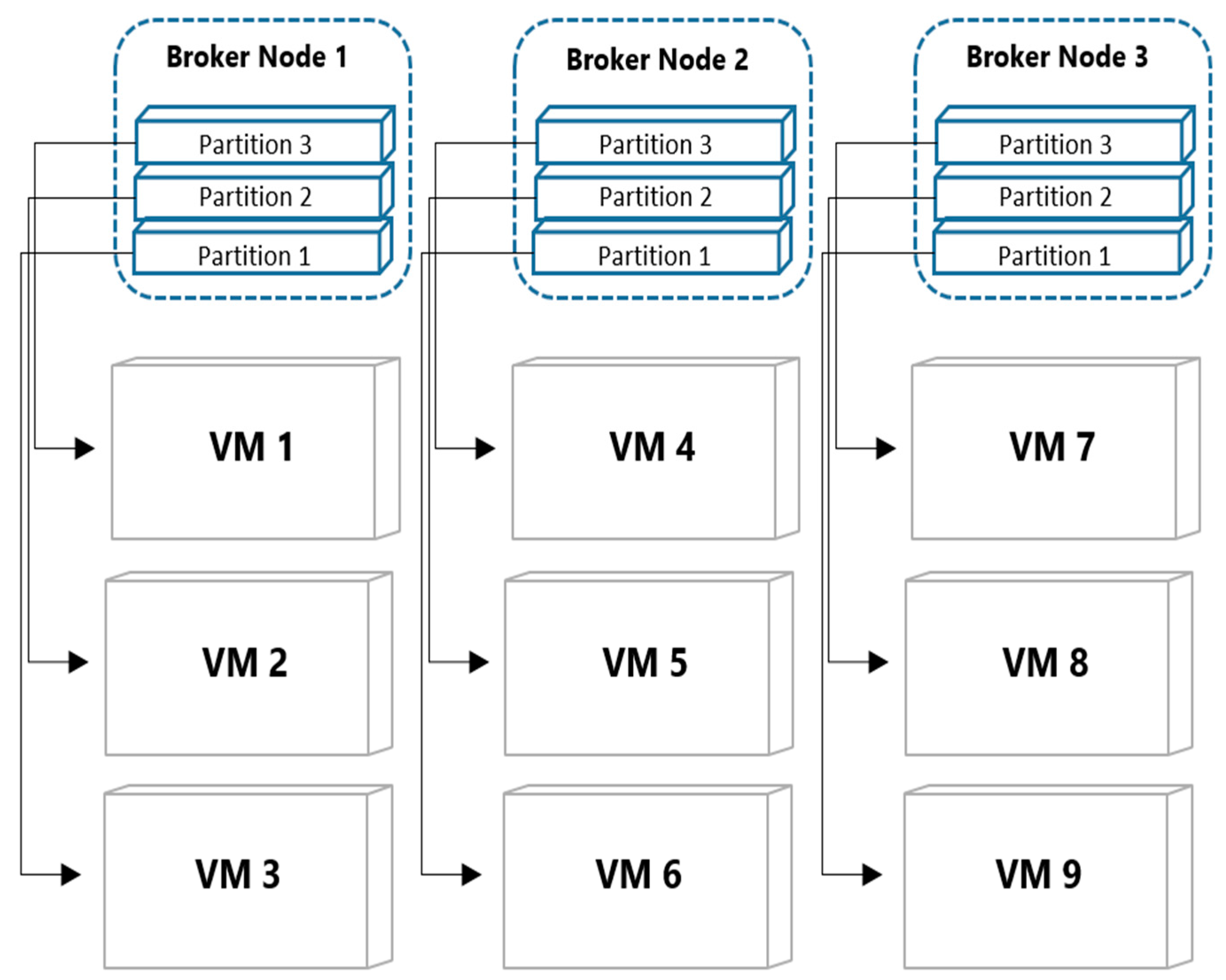
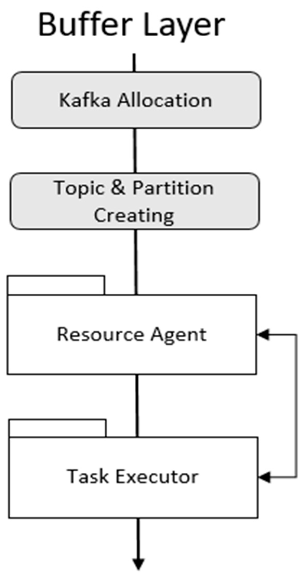
3.3. Buffer Layer

The buffer layer temporarily stores the stream data generated in real-time. One topic is a processing unit that can process a single deep learning model. In this topic, multiple broker nodes are placed to distribute the stream data accumulated in topics. In addition, multiple partitions within a single broker node provide logical storage. Having multiple partitions spreads the data evenly within one node. In the DiPLIP system, stream data is stored in the round-robin method on each node and partitions in the stream image frame. The number of broker nodes can be distributed in many ways by adjusting the number of partitions. Shows an example of a distributed environment consisting of three broker nodes and three VMs.

In Figure 3, One broker has three partitions. VM 1 connects to broker node 1, VM 2 connects to Broker Node 2, and VM 3 connects to the Broker Node 3. Each VM has ownership of three partitions, and it goes around partitions 1, 2, and 3.

As another example case, the number of VM nodes increases to 9 in Figure 4. In the figure, three VM nodes are allocated to one broker node. Figure 4 the example case of distributed environment consisting of 3 broker nodes and 9 VMs; each VM node has ownership of one partition. Since one VM node is mapped to one partition, data distribution is more efficient. Since one VM node is mapped to one partition, data distribution is more efficient than the previous example case.

3.4. Worker Layer

The worker layer consists of a resource agent and task executor. The resource agent transfers the available CPU, memory, and GPU state of the current physical node to the resource monitor of the master layer. The resource agent receives the registry location of docker image from the task controller of the master layer. The resource agent executes a docker container as a VM from docker image. VM includes a learned deep learning model and a programming virtual environment. As soon as this Docker Container is executed, it immediately accesses the buffer layer and fetches the frame to process the image.

4. Implementation

We describe the overall system implementation in detail. We will describe the process of deploying a VM image containing a deep learning model and programming a virtual environment trained through the system to a distributed environment. DiPLIP used the existing distributed resource management system, Mesos [26] using C++ language to make it a suitable model for real-time image processing. The module context for implementing this system was also included.

4.1. User Interface Layer

The user interface layer consists of four modules: resource monitoring service, resource management service, VM image management service, and model management service. The context of the module on the user interface layer is shown in Figure 5.

When the user requests the status of the currently available resource, the resource monitor contacts the resource monitor of the material layer and receives the result. When a user requests a resource to configure a buffer layer and a worker layer, the resource management service contacts the resource request on the master layer and receives the result. At this time, Kafka is automatically installed in the resources constituting the buffer layer, and the topic and partition are created according to the user’s request. When a user submits a trained deep learning model, the model management service module manages it. The model management service passes the trained model to the model submitter on the master layer.

4.2. Master Layer

The master layer consists of nine modules: resource requester, resource monitor, model submitter, resource agent manager, resource controller, topic manager, topic controller, task manager, and task controller. The context of the module on the master layer is shown in Figure 6.

For resource monitoring, the resource monitor connects to the buffer layer and the resource agent on the worker layer to exchange the results. The resource agent manager creates a resource controller whenever a VM is created and communicates with the resource agent to manage the life cycle of the VM. Each time a topic is created on the buffer layer, a topic controller is created and communicates with the resource agent on the buffer layer. The task manager creates a task controller, and each task controller communicates with the corresponding resource agent to perform the task.

4.3. Buffer Layer

The buffer layer consists of a resource agent and task executor. The resource agent receives Kafka assignment commands and deploys Kafka. When Kafka is deployed, the resource agent configures topics and partitions according to the user’s request and launches Kafka through the task executor. The context of the module on the user interface layer is shown in Figure 7.

4.4. Worker Layer

The worker layer consists of a resource agent and a task executor. When the worker node allocation is complete, the resource agent communicates with the master layer and receives the tasks. The context of the module on the user interface layer is shown in Figure 8. The resource agent manages the life cycle of each task by creating a task executor. The task executor receives the task execution command from the resource agent and executes the VM container.

4.5. Execution Scenario

DiPLIP is performed by interlocking the four layers and operates in the following order. The overall sequence of operation of DiPLIP operation procedure is shown in Figure 9.

• The user requests an available resource from the user interface layer.
• The master layer informs the user of available resources.
• The user requests the allocation of a distributed node that will serve as a buffer for real-time stream data and a worker node to perform a trained deep learning model.
• In the master layer, Kafka is deployed to distributed nodes by user’s request; it can be used as a buffer store.
• The topic of the repository is identified so that the worker node can find the buffer by name and submit the partition value for the topic.
• The user submits a deep learning trained model. In the master layer, the submitted deep learning model is packaged as a Docker image.
• The master node deploys the trained model to each worker node.
• Each worker pulls the docker image from the master node.
• The master node issues a command to execute the pulled image.

The results of this system implementation are shown in Figure 10. The input of the system is streaming data, and the output is the result of applying the deep learning model. In this study, a 30-fps web cam is used as input data and several deep learning models for object detection are used as applications. As a result, the object is detected by applying the deep learning model to the output.

5. Performance Evaluation

In order to test the performance of DiPLIP, we constructed a clustered DiPLIP system with master, worker, broker, and streaming nodes. In addition, a streaming source node is also used to deliver the image to the DiPLIP in real-time. In the streaming source node, an image of 640 × 480 resolution at 30 fps is continuously generated and transferred to the buffer layer on the DiPLIP. Since our system is designed based on the Docker Container, it only works on Linux. Finally, we evaluate the real-time distributed processing performance by submitting various trained object detection models in our system for application. On the physical node, several VM worker nodes can be created using Docker. In this experiment, up to two VM workers were created in one physical node. In the experiment, one master node, three worker nodes, three broker nodes, and one streaming node were used. The master node and the broker node used 4 GB of RAM of dual cores, and the worker node used 16 GB of RAM of quad cores. Ubuntu 16.04 OS was used for all nodes constituting DiPLIP. In addition, we will compare the distributed processing speed of the system according to the various calculation amounts by using the deep learning model [2,5] for various object detection in the experiment as an application. Object detection is the goal of all models, but the layers that make up each model are different, so the accuracy and processing speed of the results are different. All models were also trained using the COCO [27] dataset. The accuracy of each model was measured with mAP [28], and the higher the accuracy, the slower the processing speed. A summary of each model is given in [29].

Figure 11 shows the time taken to process the first 300 frames when the object detection model is inferred in the experimental environment.

Although the time taken for inference varies according to each model, it is evident that as the number of worker nodes increases, the time to process the input stream decreases. Case of 2 VMs on 2 physical worker nodes has a larger total number of VM worker nodes than case of 3 VM on 1 physical worker node, but considering that the case of 3 VMs on 1 physical worker node has a faster processing time, it is assumed that this is due to the effect of the network bandwidth. The results of this experiment show that the real-time deep learning model inference is processed faster as the number of worker nodes increases elastically.

Figure 12 shows the differential value of the unprocessed data over time on ssd mobile net model.

Data are input unprocessed for about 44 s, and after 45 s, data starts to be processed. When the data starts to be processed, it can be seen that the amount of unprocessed data decreases as the derivative value changes to a negative value. The fact that the differential value of the unprocessed data remains negative after some time elapses means that the amount being processed is greater than the amount of stream data being generated. If the differential value for the amount of unprocessed data remains positive, it means that the unprocessed value increases gradually, implying that it is time to further increase the number of worker nodes.

From the results of this experiment, it can be seen that when inferring a variety of trained deep learning models, the generated stream image can be processed at a faster rate in a distributed environment. Although the processing speed is different for each model, it can be seen that as the number of worker nodes increases, the number of frames allocated to each worker node decreases, and the overall speed increases accordingly. In addition, it can be seen through the derivative of the number of unprocessed frames that the number of processed frames increases rapidly when more worker nodes process. When the differential value of the number of unprocessed frames continues to be positive, it is implying that it is the time of expansion of the worker node.

6. Conclusions

In this paper, we presented a new distributed parallel processing platform for large-scale streaming image processing based on deep learning, called DiPLIP. It is designed to allow users to easily process large-scale stream images using a pre-trained deep learning model. It deploys a trained deep learning model by using a virtual machine Docker. It also provides a buffer layer for storing real-time streaming data temporarily, enabling reliable real-time processing. DiPLIP allows users to easily process trained deep learning models for processing real-time images in a distributed parallel processing environment at high speed through the distribution of VM containers. It supports orchestration services for performing streaming image processing based on a deep learning model on a distributed parallel environment by providing various tasks such as resource allocation, resource extension, virtual programming environment deployment, as well as a trained deep learning model and provision of automated real-time processing environment, ensuring the efficient management of distributed resources and scalable image processing.

References

- Redmon, J.; Divvala, S.; Girshick, R.; Farhadi, A. You only Look Once: Unified, Real-Time Object Detection. In Proceedings of the 2016 IEEE Conference on Computer Vision and Pattern Recognition (CVPR), Las Vegas, NV, USA, 27–30 June 2016; pp. 779–788. [Google Scholar]
- Liu, W.; Anguelov, D.; Erhan, D.; Szegedy, C.; Reed, S.; Fu, C.-Y.; Berg, A.C. SSD: Single Shot MultiBox Detector. In Computer Vision—ECCV 2016; Lecture Notes in Computer Science; Leibe, B., Matas, J., Sebe, N., Welling, M., Eds.; Springer International Publishing: Cham, Switzerland, 2016; Volume 9905, pp. 21–37. ISBN 978-3-319-46447-3. [Google Scholar]
- Liu, L.; Yang, S.; Meng, L.; Li, M.; Wang, J. Multi-scale Deep Convolutional Neural Network for Stroke Lesions Segmentation on CT Images. In Brainlesion: Glioma, Multiple Sclerosis, Stroke and Traumatic Brain Injuries; Lecture Notes in Computer Science; Crimi, A., Bakas, S., Kuijf, H., Keyvan, F., Reyes, M., van Walsum, T., Eds.; Springer International Publishing: Cham, Switzerland, 2019; Volume 11383, pp. 283–291. ISBN 978-3-030-11722-1. [Google Scholar]
- Kiran, B.R.; Roldão, L.; Irastorza, B.; Verastegui, R.; Süss, S.; Yogamani, S.; Talpaert, V.; Lepoutre, A.; Trehard, G. Real-Time Dynamic Object Detection for Autonomous Driving Using Prior 3D-Maps. In Computer Vision—ECCV 2018 Workshops; Lecture Notes in Computer Science; Leal-Taixé, L., Roth, S., Eds.; Springer International Publishing: Cham, Switzerland, 2019; Volume 11133, pp. 567–582. ISBN 978-3-030-11020-8. [Google Scholar]
- Ren, S.; He, K.; Girshick, R.; Sun, J. Faster R-CNN: Towards Real-Time Object Detection with Region Proposal Networks. IEEE Trans. Pattern Anal. Mach. Intell. 2017, 39, 1137–1149. [Google Scholar] [CrossRef] [PubMed]
- Carbone, P.; Katsifodimos, A.; Ewen, S.; Markl, V.; Haridi, S.; Tzoumas, K. Apache Flink: Stream and Batch Processing in a Single Engine. IEEE Data Eng. Bull. 2015, 36, 4. [Google Scholar]
- Shahrivari, S. Beyond Batch Processing: Towards Real-Time and Streaming Big Data. Computers 2014, 3, 117–129. [Google Scholar] [CrossRef]
- White, T. Hadoop: The Definitive Guide; O’Reilly Media, Inc.: Sebastopol, CA, USA, 2012. [Google Scholar]
- Zaharia, M.; Chowdhury, M.; Das, T.; Dave, A.; Ma, J.; McCauley, M.; Franklin, M.J.; Shenker, S.; Stoica, I. Resilient Distributed Datasets: A Fault-Tolerant Abstraction for In-Memory Cluster Computing. In Proceedings of the 9th USENIX Symposium on Networked Systems Design and Implementation, San Jose, CA, USA, 25–27 April 2012. [Google Scholar]
- Abadi, D.J.; Ahmad, Y.; Balazinska, M.; Hwang, J.-H.; Lindner, W.; Maskey, A.S.; Rasin, A.; Ryvkina, E.; Tatbul, N.; Xing, Y.; et al. The Design of the Borealis Stream Processing Engine. In Proceedings of the 2005 CIDR Conference, Asilomar, CA, USA, 4–7 January 2005. [Google Scholar]
- Stonebraker, M.; Çetintemel, U.; Zdonik, S. The 8 requirements of real-time stream processing. SIGMOD Rec. 2005, 34, 42–47. [Google Scholar] [CrossRef]
- Cherniack, M.; Balakrishnan, H.; Balazinska, M.; Carney, D. Scalable Distributed Stream Processing. In Proceedings of the 2003 CIDR Conference, Asilomar, CA, USA, 5–8 January 2003. [Google Scholar]
- Borthakur, D. The Hadoop Distributed File System: Architecture and Design. Hadoop Proj. Website 2007, 14, 21. [Google Scholar]
- Dean, J.; Ghemawat, S. MapReduce: Simplified data processing on large clusters. Commun. ACM 2008, 51, 107–113. [Google Scholar] [CrossRef]
- Condie, T.; Conway, N.; Alvaro, P.; Hellerstein, J.M.; Elmeleegy, K.; Sears, R. MapReduce Online. In Proceedings of the 7th USENIX Conference on Networked Systems Design and Implementation, San Jose, CA, USA, 28–30 April 2010. [Google Scholar]
- Toshniwal, A.; Donham, J.; Bhagat, N.; Mittal, S.; Ryaboy, D.; Taneja, S.; Shukla, A.; Ramasamy, K.; Patel, J.M.; Kulkarni, S.; et al. Storm@twitter. In Proceedings of the 2014 ACM SIGMOD International Conference on Management of Data—SIGMOD ’14, Snowbird, UT, USA, 22–27 June 2014. [Google Scholar] [CrossRef]
- Grit, L.; Irwin, D.; Yumerefendi, A.; Chase, J. Virtual Machine Hosting for Networked Clusters: Building the Foundations for “Autonomic” Orchestration. In Proceedings of the First International Workshop on Virtualization Technology in Distributed Computing (VTDC 2006), Tampa, FL, USA, 17 November 2006. [Google Scholar]
- Ranjan, R. Streaming Big Data Processing in Datacenter Clouds. IEEE Cloud Comput. 2014, 1, 78–83. [Google Scholar] [CrossRef]
- Kim, Y.-K.; Kim, Y.; Jeong, C.-S. RIDE: Real-time massive image processing platform on distributed environment. J. Image Video Proc. 2018, 2018, 39. [Google Scholar] [CrossRef]
- Kreps, J.; Narkhede, N.; Rao, J. Kafka: A Distributed Messaging System for Log Processing. In Proceedings of the 2011 ACM SIGMOD/PODS Conference, Athens, Greece, 12–16 June 2011. [Google Scholar]
- Tanenbaum, A.; Van, S.M. Distributed Systems: Principles and Paradigms; Prentice-Hall: Upper Saddle River, NJ, USA, 2007. [Google Scholar]
- Segal, O.; Colangelo, P.; Nasiri, N.; Qian, Z.; Margala, M. SparkCL: A Unified Programming Framework for Accelerators on Heterogeneous Clusters. arXiv 2015, arXiv:1505.01120. [Google Scholar]
- Merkel, D. Docker: Lightweight Linux Containers for Consistent Development and Deployment. Available online: https://www.linuxjournal.com/content/docker-lightweight-linux-containers-consistent-development-and-deployment (accessed on 24 August 2020).
- Cox, C.; Sun, D.; Tarn, E.; Singh, A.; Kelkar, R.; Goodwin, D. Serverless inferencing on Kubernetes. arXiv 2020, arXiv:2007.07366. [Google Scholar]
- Model Serving in PyTorch. Available online: https://pytorch.org/blog/model-serving-in-pyorch/ (accessed on 17 September 2020).
- Hindman, B.; Konwinski, A.; Zaharia, M.; Ghodsi, A.; Joseph, A.D.; Katz, R.; Shenker, S.; Stoica, I. Mesos: A Platform for Fine-Grained Resource Sharing in the Data Center. In Proceedings of the 8th USENIX Symposium on Networked Systems Design and Implementation, Boston, MA, USA, 30 March–1 April 2011. [Google Scholar]
- Lin, T.-Y.; Maire, M.; Belongie, S.; Hays, J.; Perona, P.; Ramanan, D.; Dollár, P.; Zitnick, C.L. Microsoft COCO: Common Objects in Context. In Computer Vision—ECCV 2014; Lecture Notes in Computer Science; Fleet, D., Pajdla, T., Schiele, B., Tuytelaars, T., Eds.; Springer International Publishing: Cham, Switzerland, 2014; Volume 8693, pp. 740–755. ISBN 978-3-319-10601-4. [Google Scholar]
- Henderson, P.; Ferrari, V. End-to-End Training of Object Class Detectors for Mean Average Precision. In Computer Vision—ACCV 2016; Lecture Notes in Computer Science; Lai, S.-H., Lepetit, V., Nishino, K., Sato, Y., Eds.; Springer International Publishing: Cham, Switzerland, 2017; Volume 10115, pp. 198–213. ISBN 978-3-319-54192-1. [Google Scholar]
- Hui, J. Object Detection: Speed and Accuracy Comparison (Faster R-CNN, R-FCN, SSD, FPN, RetinaNet and YOLOv3). Available online: https://medium.com/@jonathan_hui/object-detection-speed-and-accuracy-comparison-faster-r-cnn-r-fcn-ssd-and-yolo-5425656ae359 (accessed on 24 August 2020).
© 2020 by the authors. Licensee MDPI, Basel, Switzerland. This article is an open access article distributed under the terms and conditions of the Creative Commons Attribution (CC BY) license (http://creativecommons.org/licenses/by/4.0/).
Share and Cite
Kim, Y.-K.; Kim, Y. DiPLIP: Distributed Parallel Processing Platform for Stream Image Processing Based on Deep Learning Model Inference. Electronics 2020, 9, 1664. https://doi.org/10.3390/electronics9101664
Kim Y-K, Kim Y. DiPLIP: Distributed Parallel Processing Platform for Stream Image Processing Based on Deep Learning Model Inference. Electronics. 2020; 9(10):1664. https://doi.org/10.3390/electronics9101664
Chicago/Turabian StyleKim, Yoon-Ki, and Yongsung Kim. 2020. "DiPLIP: Distributed Parallel Processing Platform for Stream Image Processing Based on Deep Learning Model Inference" Electronics 9, no. 10: 1664. https://doi.org/10.3390/electronics9101664
APA StyleKim, Y.-K., & Kim, Y. (2020). DiPLIP: Distributed Parallel Processing Platform for Stream Image Processing Based on Deep Learning Model Inference. Electronics, 9(10), 1664. https://doi.org/10.3390/electronics9101664