Adaptive Wiener Filter and Natural Noise to Eliminate Adversarial Perturbation

Abstract

Deep neural network has been widely used in pattern recognition and speech processing, but its vulnerability to adversarial attacks also proverbially demonstrated. These attacks perform unstructured pixel-wise perturbation to fool the classifier, which does not affect the human visual system. The role of adversarial examples in the information security field has received increased attention across a number of disciplines in recent years. An alternative approach is “like cures like”. In this paper, we propose to utilize common noise and adaptive wiener filtering to mitigate the perturbation. Our method includes two operations: noise addition, which adds natural noise to input adversarial examples, and adaptive wiener filtering, which denoising the images in the previous step. Based on the study of the distribution of attacks, adding natural noise has an impact on adversarial examples to a certain extent and then they can be removed through adaptive wiener filter, which is an optimal estimator for the local variance of the image. The proposed improved adaptive wiener filter can automatically select the optimal window size between the given multiple alternative windows based on the features of different images. Based on lots of experiments, the result demonstrates that the proposed method is capable of defending against adversarial attacks, such as FGSM (Fast Gradient Sign Method), C&W, Deepfool, and JSMA (Jacobian-based Saliency Map Attack). By compared experiments, our method outperforms or is comparable to state-of-the-art methods.

1. Introduction

Computer vision is one of these fields where convolutional DNNs are usually used and commonly very effective. However, several challenges accompany the benefits of the use of DNNs. The deep neural networks (DNNs) become unreliable and insecure due to the existence of adversarial examples. Small perturbations that are difficult for humans to detect are intentionally added to the input images to cause a DNN cannot work properly [1] as shown in Figure 1. These adding visually imperceptible perturbations fail not only for image classification [2] but also object detection [3] and semantic segmentation [4]. Adversarial examples pose a serious security threat to the current commercial machine learning systems and hold back the deployment and application of the DNNs, such as driverless cars. Most existing adversarial attacks are performed by adding unstructured perturbations in the pixel-wise input space to fool the DNNs. Many security researchers consider that to be an imminent threat right now.

Recently, many scholars are beginning to make hesitant progress on this line of research. It seems there are two main methods for defending adversarial examples. One approach is improving the robustness of DNNs, training sets usually contain some adversarial examples and clean images, this is called defensive distillation. Another approach is pre-processing the input images, this operation should not affect the clean image but restore the adversarial examples to correct classification. There are a large number of published studies that expound on the view of defense methods. Stephan Zheng et al. [5] present a method of adversarial training to improve the robustness of the neural networks, while it requires many adversarial examples and an enormous amount of computing. Papernot et al. [6] proposed distillation, which improves the generalization of DNNs to defense adversarial samples crafted using the fast gradient sign method. But, unfortunately, distillation is not secure when adjusting some parameters in attacking [7]. J. Gao et al. proposed DeepCloak defense technique, a special network is added in front of the output layer to remove unnecessary features. This can provide additional security and improve the robustness of DNNs [8]. Pouya Samangouei et al. try to use Generative Adversarial Networks (GAN) for reconstructing images that correspond to adversarial examples and call “Defense-GAN”. In this method, “Defense-GAN” simulates the distribution of clean images to find a proximate output without perturbation for each input image [9]. Yue Zhou et al. propose an overall probability value (OPV) defense algorithm based on the Markov chain to mitigating the perturbation of adversarial examples. The relationship between neighbor pixels can be regarded as Markov chain, and the correlation of adjacent pixels is used as an index to judge whether the image has been perturbed or not [10]. Some latest studies focus on detecting adversarial examples directly, they either require modifying the model or acquiring adequate adversarial examples for addition training [11,12,13]. Wu et al. use recurrent occlusion attacks (ROA) to prove that the traditional machine learning method is not robust when facing the adversarial examples of the physical world, such as those generated for faces and traffic signs. At the same time, a method of defending physical adversarial examples based on adversarial training with ROA threat model is proposed [14]. Connie Kou et al. Proposed an improved method to enhance the defense based on transformation. The method only uses clean image to train an independent lightweight distribution classifier that pays close attention to the features, which output by softmax layer and can be compatible with most of the current defensive methods [15]. Chuanbiao song et al. Proposed a robust local feature adversarial training method. This method changed the focus from the global structure to the local, and used random block shuffle strategy to segment the local feature in the adversarial examples, then add it to the adversarial training [16].

Admittedly, it is unadvisable to modify the existing architecture of the CNNs. Adversarial training maybe a good choice, but it requires a large number of adversarial examples to join the training set and ceases to be effective when new attack method emerge. Even more serious is new adversarial techniques keep coming out in the last several years, for example, adversarial in 3D printing [17] and feature manipulation [18]. Unfortunately, most existing defense techniques are model-specific, which leaves a window for at-tackers to craft innovational adversarial examples.

To resolve the challenges mentioned above, we try to explore a low-cost and effective approach. The perturbation needs to be confined within a small range to make adversarial examples imperceptible. Consequently, this is very important, the information introduced by the perturbation should as little as possible. In the proposed method, we treat the adversarial example as another “normal image” and the aim is to get the corresponding degraded image in a certain range. If we add some noise and filter properly, the degraded adversarial example would be classified as a new class that different from the attack target. Meanwhile, for the legitimate image, the same operation would have little impact on the image’s semantics and keep it can be correctly classified. Theoretically, perturbation introduced by adversarial example tends to less tolerant of the denoising process than the original image information. On the other hand, we notice that some studies present state-of-the-art classifiers are robust and able to against a certain degree of distortions [19]. Thus, the adversarial example can be effectively mitigated by adding noise and filtering.

We use classic image-processing techniques such as Wiener filtering, natural noise to reduce perturbation of adversarial examples. For, all things considered, it is advisable to adopt different methods for a different type of images. A typical example: a grayscale handwritten digit generally contains hundreds of pixels, but a color image often provides a lot of pixels. This means the color image can provide larger perturbation space than a grayscale image and the perturbation strength of each should be different. Therefore, the strategy suitable for multidimensional one probably not for low-dimension sample and lead to a false positive or false negative. In short, different types of images should match the appropriate strategy pattern. The method aims to improve the generality for different kinds of images, so adaptive noise addition and filtering are enforced, we describe in Section 2.

Our contributions and impact are the following.

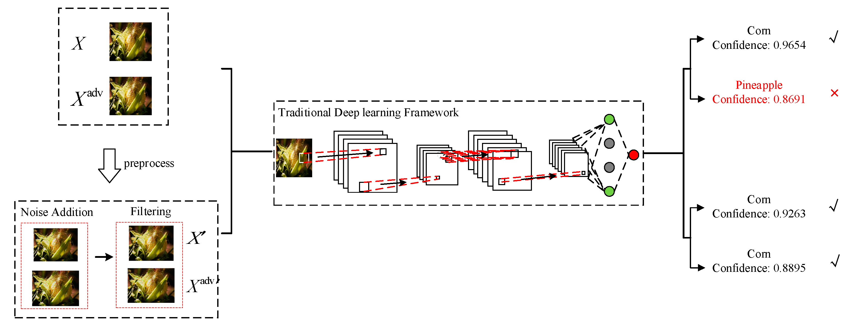
• We introduce classic image-processing techniques, such as noise addition and filtering, to degrade the image in a certain range and reduce the perturbation effect. The advantage of the classic image-processing method is easy to operate, and we properly improve the adaptive Wiener filtering technology to improve the efficiency. Adversarial examples after processing can be correctly recognized and classified.
• We deeply study the principles and the distribution of the perturbed pixels caused by the different adversarial attacks. They are not deployed regularly, but randomly distributed in the whole image. Therefore, adding natural noise, such as gaussian noise, is bound to have an impact on adversarial perturbation. A subsequent adaptive wiener filtering can be applied to soft this corruption.
• We simulate different types of attack situations (defense-unaware scenario and defense-aware scenario). Then conduct a comprehensive experimental study to demonstrate that the proposed method can effectively eliminate the perturbation in adversarial examples and achieve state-of-the-art performance.

2. Background: Adversarial Attack

In this section, we sum up the threat in deep learning by analyzing some typical adversarial attacks in computer vision. For the convenience of readers, the core technical details of the approaches are presented. Consider an image classification C and an image $x\in X, X={\left[0,1\right]}^{H\ast W\ast C}$, untargeted adversarial example $x^{\prime }$ can be defined as $x^{\prime }\in X, C\left(x\right)\ne C\left(x^{\prime }\right)$ $d\left(x,x^{\prime }\right)\le \rho$, where $d(,)$ is the dissimilarity function meanwhile $\rho \ge 0$. In practice, $d(,)$ often use Euclidean distance $d\left(x,x^{\prime }\right)=\parallel x-x^{\prime }{\parallel }_2$ or Chebyshev distance $d\left(x,x^{\prime }\right)=\parallel x-x^{\prime }{\parallel }_{\infty }$. The targeted attack is similar, but a specific target label needs to be specified., i.e., $C\left(x^{\prime }\right)=k$.

2.1. Box-Constrained L-BFGS

The perturbed images could fool deep learning models to make an error decision that was first demonstrated in paper [20]. A clean image can be denoted by ‘c’ and $I_c\in {ℝ}^m$, an additive perturbation $\mathit{\rho }\in {ℝ}^m$ would perturb the image inconspicuously. The process of solving for $\mathit{\rho }\in {ℝ}^m$ is given by Equation (1).

$$\underset{\mathit{\rho }}{\min }\parallel \mathit{\rho }{\parallel }_2 s.t. C\left(I_c+\mathit{\rho }\right)=\ell ; I_c+\mathit{\rho }\in {\left[0,1\right]}^m$$

(1)

where ‘$\ell$’ denotes the one category and $C(.)$ is the DNN classifier. Equation (2) is a hard problem and the approximate solution is sought using Box-constrained L-BFGS; decent c should satisfy the condition $C\left(I_c+\mathit{\rho }\right)=\ell$:

$$\underset{\mathit{\rho }}{\min }c\left|\rho \right|+ℒ\left(I_c+\mathit{\rho },\ell \right) s.t. I_c+\mathit{\rho }\in {\left[0,1\right]}^m$$

(2)

where $ℒ\left(.,.\right)$ computes the loss of the classifier. The result of Equation (2) has a convex loss function that satisfies the exact solution above. The computed perturbation is added to the image to make it an adversarial example.

2.2. Fast Gradient Sign Method (FGSM)

Szegedy et al. demonstrated in their paper that the adversarial training is a way of improving the robustness of deep neural networks [21]. Goodfellow et al. developed a method to efficiently generate adversarial perturbation.

$$\mathit{\rho }=ϵ\ast sign\left(\nabla \mathcal{J}\left(\theta ,I_c,\ell \right)\right)$$

(3)

where the $\nabla \mathcal{J}\left(.,.,.\right)$ computes the gradient of the cost function around the current value of the model parameters $\theta w.r.t. I_c$. sign(.) denotes the sign function and $ϵ$ is a small scalar that restricts the norm of the perturbation. Kurakin et al. in their research show that the top-1 error rate on the adversarial examples generated by FGSM is around 63–69% for $ϵ\in \left[2, 32\right]$ [22]. The computed perturbation is then subtracted from the normal images to get the adversarial examples. This attack also has an iterative version named Iterative Fast Gradient Sign Method Attack (I-FGSM). Commonly, α = ϵ/T, T refers to the number of iterations. Undoubtedly, I-FGSM has powerful damaging potential, but the transferability is poor.

$$x_0=x, x_{t+1}=x_t+\alpha \ast sign\left(\nabla \mathcal{J}\left(\theta ,I_c,\ell \right)\right)$$

(4)

2.3. Jacobian-Based Saliency Map Attack (JSMA)

This attack changes several pixels of a clean image at a time and monitors the effects of the change on the final classification. The gradients of the outputs of the network layers were used to compute the saliency map to perform monitoring. The larger value indicates a higher likelihood of fooling the DNNs, the algorithm alters the most effective pixels after the map computed. This process is repeated until the fooling succeeds or reaches the maximum limit number of altered pixels [23].

2.4. Carlini and Wagner Attacks (C&W)

Carlini and Wagner introduce a set of three adversarial attacks after defensive distillation [24]. These attacks make the perturbations imperceptible by restricting their $l_2$, $l_{\infty }$, and $l_0$ norms. Such an attack can be described as the following minimization problems.

$$\parallel x-x^{\prime }{\parallel }_2+\lambda \max \left(-\mathsf{\kappa },Z{\left(x^{\prime }\right)}_k\right)-\max \left\{Z{\left(x^{\prime }\right)}_{k^{\prime }}:k^{\prime }\ne k\right\}$$

(5)

This leads to the fact that many defense methods like defensive distillation etc. almost completely become unfruitful. Furthermore, adversarial examples generated by this algorithm also have good transitivity, which makes the computed perturbation can be used in performing black-box attacks.

2.5. Deepfool

Moosavi-Dezfooli et al. proposed a method that perturbs the clean image that is around in the region confined by the decision boundaries of the classifier and named “Deepfool” [25]. At each iteration, the algorithm computes a vector that takes the image to the boundary of the polyhedron that is obtained by linearizing the boundaries of the region in which the image resides. This process can be described as follows.

$${\rho }_{adv}\left(\widehat{k}\right)=E_x\frac{\mathsf{\Delta }\left(x;\widehat{k}\right)}{\parallel x{\parallel }_2}$$

(6)

$$\mathsf{\Delta }\left(x;\widehat{k}\right):=\underset{r}{\min }\parallel r{\parallel }_{2}subject to \widehat{k}\left(x+r\right)\ne \widehat{k}\left(x\right)$$

(7)

where $\mathsf{\Delta }\left(x;\widehat{k}\right)$ denotes the robustness of $\widehat{k}$ at point x, r denotes the perturbation, $\widehat{k}\left(x\right)$ is the estimated label, and $E_x$ is the expectation over the distribution of the data.

3. Related Work

Transformation-based defenses are rarely explored development in adversarial defense, because the challenge facing most transformation-based defenses is the reduced normal images may cause the decrease of accuracy. This has limited the practical use of transformation method. We have a hypothesis that not all regions of a given image are useful to a classifier. Besides, foveation-based methods also not a better choice and it can be easily fooled by finding an adversarial perturbation within the object bounding box. So, it is not advisable to restrict only modifying a certain location of the input. Recent studies suggested that most deep classifiers are robust to the presence of natural noise [26] such as the noise mentioned in Section 4.1.

Distribution of Attacks

We conduct an experiment and the aim is to explore the distribution of the different adversarial attacks. The result shows that most attacks search the whole image region for adversarial perturbations without regard the location of the major area. This is especially true for attacks which give little constraint on the total number of pixels perturbed. We show the average spatial distribution of perturbations for some known attacks and the major region to make the comparison, as shown in Figure 2. We can clearly see that most attacks add adversarial perturbation to the whole image plane. This is different from the CNNs for image classification, because the CNNs only focuses on the heatmap of the image. This is especially true for attacks that do not limit the total number of pixels to be perturbed. Based on this investigation, we try to explore the possibility of adding random natural noise to affect adversarial perturbation and dissolve them all to restore a “pure” image through adaptive filtering.

4. Methodology

The main idea behind our designs is to use natural noise damage the elaborate perturbation and introduce image processing techniques to eliminate the adversarial effect as far as possible. As described in the previous section, through elaborately superimposing dressing on a clean image, it easily becomes an adversarial example. From viewpoint of a make-up artistry, an adversarial example can be viewed as made-up face, what we need to do is to develop a suitable “makeup remover” that restores genuine visage.

Take for example the FGSM adversarial example, it can be viewed as an additive noise whose amplitude is $\epsilon$. In the ideal situation, we want to reconstruct a clean image form an adversarial example, nevertheless, achieving this is very difficult. Because we cannot determine the exact perturbation location and strength. A new way of thinking is seeking to reconstruct an adversarial example, i.e., we want to convert adversarial example to a new image that can be correctly classified, the method framework as shown in Figure 3.

Rightfully so, a benign sample classification does not change while maintaining almost the same confidence after the conversion. As mentioned earlier, state-of-the-art DNN image classifiers can tolerate a certain degree of distortion, although they would misclassify the adversarial examples. As Figure 4 illustrates, the original image is classified as Golden retriever by GoogleNet with 0.9833 confidence. After being either grayed, resized, compressed, or blurred, these transformed images still can be correctly classified with high confidence.

The noise can affect the clean image, and so is the adversarial example. Base on the above analyses, it is true that some details in the image may be lost, but the classifiers can still output the correct classification for a filtered image. It is important that we add natural noise to adversarial examples to damage the elaborate perturbation, however, we cannot imply that the perturbation follows certain distributions. S.M. Moosavi-Dezfooli et al. indicated in their paper that the perturbation may differ largely from one attack to another [22]. In reality, we may not accurately know what the adversary uses and the detailed perturbation features means. Many times, randomness is the actual feature of perturbation, this makes it difficult for us to make a prediction.

4.1. Natural Noise

Image noise refers to unnecessary or redundant interference information in an image. Noise is theoretically defined as a random error that is unpredictable in the natural environment. In digital imaging processing, Gaussian white noise, salt & pepper noise, Poisson noise, and multiplicative noise are common noise sources. The power spectral density of Gaussian white noise obeys uniform distribution while the amplitude distribution obeys Gaussian distribution, in the experiment the parameter settings are $\mu =0$ and $\sigma =0.01$. Salt & pepper noise refers to two kinds of noise, one is salt noise (white, grayscale is 255), the other is pepper noise (black, grayscale is 0). The former is high grayscale noise, the latter is low grayscale noise, two kinds of noise generally appear at the same time, in the experiment the noise density setting is $d=0.05$. Poisson noise also known as shot noise, is a basic form of uncertainty associated with the measure of light and inherent to the quantized nature of light, in the experiment, the parameter settings are default. Multiplicative noise is a type of signal- dependent noise and the variance of the noise is a function of the signal amplitude, in the experiment the variance parameter setting is $\sigma =0.05$. In the following experiment section, we conduct a comparative experiment to compare the effects of different noises.

4.2. Adaptive Wiener Filtering

Adaptive wiener filtering adjusts the output of the filter according to the local variance of the image. Its ultimate goal is to minimize the mean square error between the restored image and the original image. The filtering effect of this method is better than the other filters, and it is very useful for preserving the edges and high-frequency regions of the image. In addition, we made some adjustments. On the one hand, we apply different window alternatives to deal with diverse scenarios and automatically pick the best-possible one. On the other hand, at smooth regions, the center sample in the moving window should be neglected to suppress subjectively annoying singularities but properly used in rough regions.

Consider the filtering of images corrupted by signal-intendent noise, the problem can be modeled as

$$y\left(i,j\right)=x\left(i,j\right)+n\left(i,j\right)$$

(8)

where $y\left(i,j\right)$ is the noisy measurement, $x\left(i,j\right)$ is the noise-free image and $n\left(i,j\right)$ is additive noise. The aim is to remove noise or “denoise” $y\left(i,j\right)$. For a pixel in the image, the mean and variance of the pixel in different window sizes, such as ${\left(3+2i\right)}^2,i=0,1,2,3$, are compared, and then the window is used by the minimum average value is taken as the final processing window, as shown in Figure 5. The filter template can be selected adaptively according to different regions. The small window filter is used in the detail part, and the large window filter is used in the smooth area, which can improve the efficiency and retain the edges and texture parts. The following formula is used to process the pixels and get the output results.

$$r\left(i,j\right)=\mu +\left(1-q+∆\right)\ast \left(s\left(i,j\right)-\mu \right)$$

(9)

$$q=\frac{{\sigma }_{avg}}{{\sigma }_{var}+1}$$

(10)

$$∆=\frac{{\sigma }_{var}}{{\sigma }_{avg}+{\sigma }_{max}+1}$$

(11)

$s\left(i,j\right)$ means the original pixel, $s\left(i,j\right)$ means the output pixel, ${\sigma }_{avg}$ is the mean of the variance sum of all pixels in the selected window, ${\sigma }_{var}$ is the variance of the current pixel, and ${\sigma }_{max}$ is the maximum variance of all pixels in the image.

This leads to considerable improvement and the result of the inner window can be reused to larger outside window in the computing. We process both clean image and adversarial example, the result as shown in Figure 6. In the experiment part of the paper, we conduct a comparative experiment to compare the adaptive wiener filter with other filters.

5. Experiment

The images have been misclassified by the DNN classifier are little significance. Therefore, we randomly selected 20,000 images correctly classified by all considered networks from the ImageNet, which is a large-scale dataset of labeled color images. These images are of size 299 × 299 × 3 and form our test dataset. The experiment performs on publicly available networks, includes Inception-v4 [27], Resnet-v2 of 101 layers [28] and vgg16 [29]. Inception V4 is the fourth version of the neural network architecture proposed by Google in 2016. Compared with the previous version, it improves the conv-pooling results, increases the depth of the network, and significantly reduces the Top1 error and top-5 error. VGG was proposed by the visual geometry group of Oxford on ILSVRC 2014. The model participated in the ImageNet classification and positioning challenge in 2014 and achieved excellent results. VGG include two structures, vgg16 and vgg19. There is no essential difference between them except the depth of the network. Resnet-v2 (Residual Neural Network) is proposed by five Chinese scholars from Microsoft Research Institute. Through the use of Resnet unit, 152-layer neural network was successfully trained and won the championship in ILSVRC 2015. The structure of Resnet-v2 can accelerate the training of a neural network very quickly, and the accuracy of the model is also greatly improved. Weights for each model can be found in TensorFlow repository in GitHub, and we list the link in the Appendix A section. We call them “target model”.

There we add two layers before the “target model”. For the noise addition layer, we attempt to add different types of noise to input data and treat clean images and adversarial examples equally. For the filtering layer, we try to adopt different filter types to process the noisy images and carry out a comparative analysis. After the above steps, these images are sent to DNN classifiers for categorizing. The combination we call them “defense model”.

The perfect attack for an adversary is considering all possible patterns of the defense model when generating adversarial examples. The added noise addition layer and the filtering layer could lead to the process of attack take a long time or not convergence that greatly reduce the success rate of the adversary. In the experiment, the defense models and the target models are the same except for the additional two layers.

5.1. Adversarial Example Generation

For FGSM attack, setting parameter $\epsilon$ value is critical. There is a positive correlation between the size of $\epsilon$ and the success rate of adversarial examples. If the value of $\epsilon$ is large, the added perturbation would be too obvious. In practice, 1/255 or 2/255 are reasonable optional values for ImageNet. For Deepfool attack, there is an available open access project on the GitHub. The algorithm finds the nearest classification boundary iteratively to complete the deception. For C&W attack, it has three modes to choose, one is to limit the number of pixels to be altered, the other is to limit the overall extent of the perturbation, another is limiting the maximum number of perturbed pixels.

For instance, C&W $l_2$ attack craft adversarial examples with much lower distortion than FGSM and $\mathsf{\kappa }$ we set respectively 0, 0.5, 1.0, 2.0, and 4.0 in the experiment. For JSMA and L-BFGS attacks, we do not make special settings, but use the original parameters in the algorithm. It should be noted that JSMA and L-BFGS are perceptible perturbations, they limit the number of altered pixels but not the amplitude of the pixels. There are some differences can be clearly found between the adversarial examples generated in this way and the normal image, but it still has reference significance.

5.2. Legitimate Samples Test

In this section, we attempt to test the performance of noise addition and adaptive wiener filtering on legitimate Images. We randomly select 10,000 clean images to add different kinds of noise and filtering, they are classic image-processing techniques. The DNN classifiers are Inception-v4, Resnet-v2 of 101 layers and vgg16.

The result as shown in

Table 1. The impact on classification of clean images of different combinations of noise addition and filtering (Inception v4/ Resnet-v2 of 101/ vgg16).

Filter	Gaussian White Noise	Salt & Pepper Noise	Poisson Noise	Multiplicative Noise
Gaussian	98.17%/98.26%/98.64%	97.16%/97.69%/97.53%	98.29%/97.55%/96.94%	99.03%/98.14%/98.33%
Median	99.19%/98.61%/97.92%	99.46%/98.97%/98.86%	98.49%/98.25%/98.47%	99.24%/99.13%/99.02%
Mean	98.87%/98.89%/98.49%	99.03%/98.89%/98.43%	98.60%/97.68%/98.29%	99.14%/98.71%/98.66%
Bilateral	99.34%/99.01%/99.12%	99.21%/98.56%/98.74%	98.93%/98.61%/98.59%	99.9%/98.84%/98.73%
KNN	97.37%/97.11%/96.86%	97.67%/96.83%/96.93%	98.87%/98.38%/98.14%	98.99%/99.04%/98.59%
High-pass	8.17%/6.26%/7.14%	7.87%/7.62%/7.34%	9.69%/8.89%/9.64%	6.95%/7.07%/6.81%
Low-pass	98.77%/98.52%/98.71%	98.41%/98.15%/98.27%	98.65%/98.11%/98.23%	98.97%/98.95%/98.78%
Adaptive wiener	99.36%/99.13%/99.08%	99.43%/99.26%/99.19%	99.29%/99.06%/99.11%	99.49%/99.32%/99.34%

, it is fairly clear that the combination of Multiplicative noise and adaptive wiener filtering achieves the best performance because this combination has the least effect on the classification of legitimate images in different DNN classifiers. Simultaneously, the DNN classifier Inception v4 has better robustness, it has the highest accuracy and mean confidence of an image generated by the combination of these different techniques. In addition, it is not hard to see the combination of high-pass filter and noise achieve the worst performance, and the performance for other combinations is incredibly close but the adaptive wiener filter has weak advantage.

Next, we random choose 10,000 different kinds of adversarial examples generated based on Inception v4 instead clean images and perform the experiment again (target model is also Inception v4), the result as shown in

Table 2. The performance of different combination of noise addition and filtering on adversarial examples (correct classification rate).

Filter	Gaussian White Noise	Salt & Pepper Noise	Poisson Noise	Multiplicative Noise
Gaussian	65.71%	69.16%	58.79%	63.84%
Median	51.49%	56.47%	52.31%	56.53%
Mean	67.54%	61.29%	62.63%	66.87%
Bilateral	46.92%	53.38%	48.43%	49.45%
KNN	36.41%	40.26%	47.31%	39.68%
High-pass	0%	0%	0%	0%
Low-pass	59.83%	59.67%	56.95%	58.67%
Adaptive wiener	76.58%	81.29%	74.94%	93.87%

.

We can clearly see from Table 2 that the combination of multiplicative noise and adaptive wiener filter achieve the best performance, other combinations also have some effect but not as good as the former. In the experiment, we notice that about 10% adversarial examples could be correctly classified when adding the noise, the perturbation of the other adversarial examples somehow affected as well. After filtering, most adversarial examples can be correctly classified and the reason for misclassification we analyze in the discussion and limitation.

5.3. Different Attack Scenarios Test

In this section, we evaluate the proposed method on different attack scenarios. Considering the actual situation, we assume two scenarios, defense-unaware attack and defense-aware attack. In defense-unaware scenario, we assume the adversary does not know the exact internal structure of the model, especially the noise addition layer and adaptive wiener filtering layer. In this case, the adversarial can only generate adversarial examples on the “target model”. The defense-unaware test result as shown in

Table 3. The results of the proposed method under the defense-unaware scenarios.

Models	Inception-v4		Resnet-v2		Vgg16
	Target Model	Defense Model	Target Model	Defense Model	Target Model	Defense Model
FGSM ($\epsilon =1/255$)	3.11%	95.63%	2.89%	94.59%	3.27%	95.93%
FGSM ($\epsilon =2/255$)	1.79%	94.39%	2.08%	93.96%	2.147%	94.65%
C&W $l_2$ ($\mathsf{\kappa }=0.0$)	1.36%	91.62%	1.59%	92.16%	2.25%	93.27%
C&W $l_2$ ($\mathsf{\kappa }=0.5$)	1.33%	90.26%	1.43%	91.37%	1.98%	92.69%
C&W $l_2$ ($\mathsf{\kappa }=1.0$)	1.21%	90.53%	1.34%	91.78%	1.88%	91.53%
C&W $l_2$ ($\mathsf{\kappa }=2.0$)	1.14%	90.03%	1.11%	91.28%	1.58%	91.39%
C&W $l_{\infty }$ ($\mathsf{\kappa }=4.0$)	1.29%	92.75%	1.18%	94.03%	1.59%	91.17%
Deepfool	2.87%	96.33%	1.89%	97.63%	2.65%	96.48%
JSMA	2.56%	97.24%	2.37%	97.82%	2.57%	96.77%
L-BFGS	2.81%	95.86%	2.51%	96.79%	2.66%	96.01%

.

In defense-aware attack, we assume the adversary detects the existence of the defense model i.e., noise addition layer and adaptive wiener filtering layer, but cannot acquire a detailed work mechanism. In the extreme, we make another assumption, the adversary knows the entire internal structure, i.e., the model is a white-box. The adversary can exploit the vulnerability of the detection method to perform an attack and ensure the adversarial examples of every optimization and their denoised version are classified as the same thing. This may greatly increase the success rate. We refer to the Reference [30] and launch a defense-aware attack on 10,000 ImageNet test samples. The defense-aware test result as shown in

Table 4. The results of the proposed method under the defense-aware scenarios.

Models	Inception-v4		Resnet-v2		Vgg16
	Target Model	Defense Model	Target Model	Defense Model	Target Model	Defense Model
FGSM ($\epsilon =2/255$)	1.81%	79.12%	1.98%	77.57%	186%	79.52%
C&W $l_2$ ($\mathsf{\kappa }=1.0$)	2.37%	62.84%	2.17%	64.73%	2.17%	68.13%
C&W $l_{\infty }$ ($\mathsf{\kappa }=4.0$)	1.97%	66.27%	1.87%	67.88%	1.51%	65.85%
Deepfool	2.83%	71.39%	2.06%	72.82%	2.36%	75.76%
JSMA	2.26%	81.78%	2.27%	82.34%	2.99%	78.04%
L-BFGS	2.76%	74.99%	2.86%	76.38%	2.45%	75.61%

.

5.4. Comparison Experiment

In this section, we conduct a comparison with the methods based on generative adversarial network [31], JPEG compression [32], image hybrid transformation method [33], and spatial smoothing filter [34], result as shown in

Table 5. The results of performance comparison experiment.

	JPEG	APE-GAN	Cropping + TVM + Quilting	Spatial Smoothing Filter	The Proposed Method
FGSM	65.63%	50.91%	71.52%	89.61%	94.93%
C&W	71.85%	73.92%	70.51%	85.15%	91.74%
Deepfool	71.88%	54.15%	71.47%	88.76%	90.68%
JSMA	73.8%	62.26%	68.19%	86.54%	92.44%
L-BFGS	72.9%	61.71%	70.16%	87.33%	93.79%
Defense-aware	11.6%	0%	0%	32.61%	53.15%

. The target model we choose Inceptionv4, and test all methods under defense-unaware scenario and defense-aware scenario. Because different paper targets both dissimilar $\left|L_P\right|$ norms and various perturbation magnitudes. To present a fair comparison across the methods mentioned above, it is advisable to measure the fraction of images that are no longer misclassification after the transformation.

The results are in terms of top-1 accuracy, as this matches the objective of the adversary. Compared with other classification schemes, our method has better performance under defense-unaware scenarios. Meanwhile, in extreme case, the proposed method can achieve over 53% success rate when meet defense-aware attacks.

5.5. Discussion and Limitation

In general, the proposed method can work together better with most DNN classifiers and improve their security. One other thing to note is there are some exceptions in the experiment caused by anomalous images. One scenario is an image contains too many objects, the other is unclear images as Figure 7. They can be classified correctly but have low confidence. Fortunately, these images are very few and hardly impact the performance. To solve this problem, we believe the top five predictions better than the top one with the highest confidence. It should be acknowledged that our approach is determined to be effective for most adversarial attacks. Because of the randomness of natural noise and may appear in any position of the image plane, such as Gaussian noise, the elaborate adversarial perturbations are inevitably affected by them. Subsequent filtering operation can further soft these adversarial changes. Even if all the security parameters of the defense system are exposed, the strategy can still play a certain defense effect. However, if the adversary can use as few perturbated pixels as possible to generate adversarial samples, and these perturbed pixels are concentrated in the local rather than the whole image plane. In this case, it is possible to penetrate the defense system, but this will significantly increase the cost of the adversary.

6. Conclusions

In this paper, we treat adversarial examples as “make-up face” and develop a suitable “makeup remover”, multiplicative noise and adaptive wiener filter, to restore their original features and achieve a good result. Certainly, there are also a lot of techniques have been developed to defend the adversarial examples in DNNs, but most of them require prior knowledge of attack methods or modify the existing models. In this paper, we demonstrate that most of the adversarial attacks add perturbation to the whole image plane, rather than only the heatmap region. Therefore, adding natural noise to the whole pixel plane can directly cover a certain number of disturbed pixels, making the noise distribution of the image close to the conventional noise to some extent, and can be easily eliminated by the filter. When the perturbated pixels are removed to a certain proportion, the adversarial examples can be classified normally. Through different combinations of experiments, it is admitted that the multiplicative noise and adaptive wiener filter can be used as “makeup remover” to eliminate the perturbations and the combination is better than other methods. The most important is the proposed method requires little prior knowledge and can work seamlessly together with existing DNN models. Through investigation and experiment, we find an adaptive Wiener filter which is more suitable for joint spatial-frequency analysis. For low-frequency and high-frequency regions of the image, adaptive adjustment strategy and quantization technology are more suitable for denoising. Through both defense-unaware and defense-aware test, it is clear that our method achieves good performance to eliminate adversarial perturbations. The comparison with existing methods in the experiment proves our method has obvious advantages. Moreover, the compatibility of our method is good and can combine with other defense techniques. Inspired by this, it is promising to segment an adversarial example into several regions and find the one which contains as much information as possible. In addition, there are many other image processing techniques, such as image segmentation [35], which can be leveraged to mitigate adversarial examples. In follow-up work, we will investigate more image processing techniques to find more usable and potent methods for defense-aware attacks. Admittedly, the arm race between adversaries and defenders will never stop.

References

1. Zhang, K.; Liang, Y.; Zhang, J.; Wang, Z.; Li, X.; Zhanga, J. No one can escape: A general approach to detect tampered and generated image. IEEE Access 2019, 7, 129494–129503. [Google Scholar] [CrossRef]
2. Liu, Y.; Chen, X.; Liu, C.; Song, D. Delving into transferable adversarial examples and black-box attacks. arXiv 2016, arXiv:1611.02770. [Google Scholar]
3. Xie, C.; Wang, J.; Zhang, Z.; Zhou, Y.; Xie, L.; Yuille, A. Adversarial examples for semantic segmentation and object detection. In Proceedings of the International Conference on Computer Vision, Venice, Italy, 22–29 October 2017; pp. 1378–1387. [Google Scholar]
4. Fischer, V.; Kumar, M.C.; Metzen, J.H.; Brox, T. Adversarial examples for semantic image segmentation. arXiv 2017, arXiv:1703.01101. [Google Scholar]
5. Zheng, S.; Song, Y.; Leung, T.; Goodfellow, I. Improving the robustness of deep neural networks via stability training. In Proceedings of the 2016 IEEE Conference on Computer Vision and Pattern Recognition, Las Vegas, NV, USA, 27–30 June 2016; pp. 4480–4488. [Google Scholar]
6. Papernot, N.; McDaniel, P.; Wu, X.; Jha, S.; Swami, A. Distillation as a defense to adversarial perturbations against deep neural networks. In Proceedings of the 2016 IEEE Symposium on Security and Privacy (SP), San Jose, CA, USA, 22–26 May 2016; pp. 582–597. [Google Scholar]
7. Carlini, N.; Wagner, D. Defensive distillation is not robust to adversarial examples. arXiv 2016, arXiv:1607.04311. [Google Scholar]
8. Gao, J.; Wang, B.; Lin, Z.; Xu, W.; Qi, Y. DeepCloak: Masking deep neural network models for robustness against adversarial samples. arXiv 2017, arXiv:1702.06763. [Google Scholar]
9. Samangouei, P.; Maya, K.; Rama, C. Defense-gan: Protecting classifiers against adversarial attacks using generative models. arXiv 2018, arXiv:1805.06605. [Google Scholar]
10. Zhou, Y.; Hu, X.; Wang, L.; Duan, S.; Chen, Y. Markov Chain Based Efficient Defense Against Adversarial Examples in Computer Vision. IEEE Access 2019, 7, 5695–5706. [Google Scholar] [CrossRef]
11. Xu, W.; Evans, D.; Qi, Y. Feature squeezing: Detecting adversarial examples in deep neural networks. arXiv 2017, arXiv:1704.01155. [Google Scholar]
12. Metzen, J.H.; Genewein, T.; Fischer, V.; Bischoff, B. On detecting adversarial perturbations. arXiv 2017, arXiv:1702.04267. [Google Scholar]
13. Grosse, K.; Manoharan, P.; Papernot, N.; Backes, M.; McDaniel, P. On the (Statistical) detection of adversarial examples. arXiv 2017, arXiv:1702.06280. [Google Scholar]
14. Wu, T.; Tong, L.; Vorobeychik, Y. Defending against physically realizable attacks on image classification. arXiv 2019, arXiv:1909.09552. [Google Scholar]
15. Kou, C.; Lee, H.K.; Chang, E.-C.; Ng, T.K. Enhancing transformation-based defenses against adversarial attacks with a distribution classifier. arXiv 2019, arXiv:1906.00258. [Google Scholar]
16. Song, C.; He, K.; Lin, J.; Wang, L.; Hopcroft, J.E. Robust local features for improving the generalization of adversarial training. arXiv 2019, arXiv:1909.10147. [Google Scholar]
17. Athalye, A.; Sutskever, I. Synthesizing robust adversarial examples. arXiv 2017, arXiv:1707.07397. [Google Scholar]
18. Wang, S.; Chen, S.; Chen, T.; Nepal, S.; Rudolph, C.; Grobler, M. Generating semantic adversarial examples via feature manipulation. arXiv 2020, arXiv:2001.02297. [Google Scholar]
19. Goodfellow, I.; Lee, H.; Le, Q.V.; Saxe, A.; Ng, A.Y. Measuring invariances in deep networks. In Proceedings of the Advances in Neural Information Processing Systems, Vancouver, BC, Canada, 7–10 December 2009; pp. 646–654. [Google Scholar]
20. Szegedy, C.; Zaremba, W.; Sutskever, I.; Bruna, J.; Erhan, D.; Goodfellow, I.; Fergus, R. Intriguing properties of neural networks. arXiv 2014, arXiv:1312.6199. [Google Scholar]
21. Goodfellow, I.J.; Shlens, J.; Szegedy, C. Explaining and harnessing adversarial examples. arXiv 2015, arXiv:1412.6572. [Google Scholar]
22. Kurakin, A.; Goodfellow, I.; Bengio, S. Adversarial machine learning at scale. arXiv 2017, arXiv:1611.01236. [Google Scholar]
23. Papernot, N.; McDaniel, P.; Jha, S.; Fredrikson, M.; Celik, Z.B.; Swami, A. The limitations of deep learning in adversarial settings. In Proceedings of the 2016 IEEE European Symposium on Security and Privacy, Saarbrucken, Germany, 21–24 March 2016; pp. 372–387. [Google Scholar]
24. Carlini, N.; Wagner, D. Towards evaluating the robustness of neural networks. arXiv 2016, arXiv:1608.04644. [Google Scholar]
25. Moosavi-Dezfooli, S.-M.; Fawzi, A.; Frossard, P. DeepFool: A simple and accurate method to fool deep neural networks. In Proceedings of the 2016 IEEE Conference on Computer Vision and Pattern Recognition (CVPR), Las Vegas, NV, USA, 27–30 June 2016; pp. 2574–2582. [Google Scholar]
26. Diamond, S.; Sitzmann, V.; Boyd, S.; Wetzstein, G.; Heide, F. Dirty pixels: Optimizing image classification architectures for raw sensor data. arXiv 2017, arXiv:1701.06487. [Google Scholar]
27. Szegedy, C.; Ioffe, S.; Vanhoucke, V.; Alemi, A. Inception-v4 inception-resnet and the impact of residual connections on learning. arXiv 2017, arXiv:1602.07261. [Google Scholar]
28. He, K.; Zhang, X.; Ren, S.; Sun, J. Identity mappings in deep residual networks. arXiv 2016, arXiv:1603.05027. [Google Scholar]
29. Karen, S.; Zisserman, A. Very deep convolutional networks for large-scale image recognition. arXiv 2014, arXiv:1409.1556. [Google Scholar]
30. Carlini, N.; Wagner, D. Adversarial examples are not easily detected: By passing ten detection methods. arXiv 2014, arXiv:1409.1556. [Google Scholar]
31. Jin, G.; Shen, S.; Zhang, D.; Dai, F.; Zhang, Y. APE-GAN: Adversarial perturbation elimination with GAN. arXiv 2017, arXiv:1705.07263. [Google Scholar]
32. Nilaksh, D.; Shanbhogue, M.; Chen, S.-T.; Hohman, F.; Li, S.; Chen, L.; Kounavis, M.E.; Chau, D.H. Shield: Fast, practical defense and vaccination for deep learning using jpeg compression. arXiv 2014, arXiv:1802.06816. [Google Scholar]
33. Guo, C.; Rana, M.; Cisse, M.; van der Maaten, L. Countering adversarial images using input transformations. arXiv 2017, arXiv:1711.00117. [Google Scholar]
34. Liang, B.; Li, H.; Su, M.; Li, X.; Shi, W.; Wang, X. Detecting adversarial image examples in deep neural networks with adaptive noise reduction. IEEE Trans. Dependable Secur. Comput. 2019, 1, 99. [Google Scholar] [CrossRef] [Green Version]
35. Dougherty, E.R. Digital Image Processing Methods; CRC Press: Boca Raton, FL, USA, 2020. [Google Scholar]
Publisher’s Note: MDPI stays neutral with regard to jurisdictional claims in published maps and institutional affiliations.
Figure 1. An adversarial example crafted for Inception v3.
Electronics 09 01634 g001
Figure 2. Visualization showing average location in the image where perturbation is added by an attacker.
Electronics 09 01634 g002
Figure 3. The adversarial perturbation elimination framework.
Electronics 09 01634 g003
Figure 4. The DNN classifiers has strong robustness to transformed images.
Electronics 09 01634 g004
Figure 5. Wiener filter template adaptive selection.
Electronics 09 01634 g005
Figure 6. The effect of adaptive wiener filter on clean image and adversarial example.
Electronics 09 01634 g006
Figure 7. False classification by anomalous image.
Electronics 09 01634 g007