Abstract
With the rapid development of the Internet, malware traffic is seriously endangering the security of cyberspace. Convolutional neural networks (CNNs)-based malware traffic classification can automatically learn features from raw traffic, avoiding the inaccuracy of hand-design traffic features. Through the experiments and comparisons of LeNet, AlexNet, VGGNet, and ResNet, it is found that LeNet has good and stable classification ability for malware traffic and normal traffic. Then, a field programmable gate array (FPGA) accelerator for CNNs-based malware traffic classification is designed, which consists of a parameterized hardware accelerator and a fully automatic software framework. By fully exploring the parallelism between CNN layers, parallel computation and pipeline optimization are used in the hardware design to achieve high performance. Simultaneously, runtime reconfigurability is implemented by using a global register list. By encapsulating the underlying driver, a three-layer software framework is provided for users to deploy their pre-trained models. Finally, a typical CNNs-based malware traffic classification model was selected to test and verify the hardware accelerator. The typical application system can classify each traffic image from the test dataset in 18.97 μs with the accuracy of 99.77%, and the throughput of the system is 411.83 Mbps.
1. Introduction
With the rapid development of computer network technology, the Internet is a part of people’s everyday lives, and it has been widely used in various fields such as the economy, military, education, and so on. Internet is a double-edged sword similar to some other technology: it promotes the rapid development of the social economy on one hand, but it brings unprecedented challenges on the other hand. Malware traffic refers to the malicious part in network traffic, including network attacks, business attacks, malicious crawlers, etc. In the open environment of the Internet, malware traffic has become a new criminal tool that not only seriously affects the stability of the Internet, it also causes economic losses and even seriously threatens national security [1]. According to Computer Economics, financial loss due to malware attack has grown from $3.3 billion in 1997 to $13.3 billion in 2006. Recently in 2016, two WannaCry ransomware attacks crippled the computers of more than 150 countries, causing financial damage to different organizations. In 2016, Cybersecurity Ventures3 estimated that the total damage due to malware attacks was $3 trillion in 2015, and it is expected to reach $6 trillion by 2021 [2]. Network traffic contains a lot of valuable information, as it is the most basic component of transmission and interaction in cyberspace. It is of great significance to enhance network stability, improve anti attack ability, and maintain information security by detecting and intercepting malware traffic in time.
Traditional traffic classification methods can be divided into four categories: port-based, deep packet inspection (DPI)-based, statistical-based, and behavior-based [3]. The accuracy of port-based methods is low. DPI-based methods can not process encrypted traffic and have high computational complexity. Most research studies focus on statistical-based methods and behavior-based methods, both of which are based on the idea of machine learning. These two methods do not need to check the port or analyze the traffic, they are also applicable to encrypted traffic, and the complexity of the calculations is relatively low. However, there is the same problem in the two methods: it is too difficult to design proper feature sets that can accurately reflect the characteristics of different traffic; meanwhile, the quality of the feature sets directly affects the classification performance.
Representation learning is a new rapidly developing machine learning approach in recent years that automatically learns features from raw data and to a certain extent has solved the problem of hand-designing features [4]. Especially, the deep learning method, which is a typical approach of representation learning, has achieved very good performance in many domains including image classification and speech recognition [5,6]. Deep learning is a kind of machine learning technology that is an extension of representation learning; it was proposed by Geoffrey Hinton in 2006 [7]. The convolutional neural networks (CNNs) model is one of many deep learning architectures. In the last two years, the CNNs model has become one of the research hotspots because of its good performance in image classification and object detection. Traffic characteristics can be automatically learned from the original data by using CNNs [8]. There is no need to manually extract features from traffic; instead, CNNs take raw traffic data as images, so as to avoid the problems of designing proper feature sets. The CNNs model can be used to perform image classification, which is a common task for CNNs [9]. Finally, the goal of malware traffic classification was achieved.
However, with the development of CNNs, the number of hidden layers in the neural network have gradually increased, and the number of parameters has also become larger. As a result, computation and power consumption increase further, which limits the application of CNNs-based malware traffic classification in portable devices. Therefore, research studies on the hardware acceleration of CNNs-based malware traffic classification are necessary.
Considering the problems above, CNNs-based methods are constructed to evaluate their ability for malware traffic classification, and a field programmable gate array (FPGA) accelerator for CNNs-based malware traffic classification is designed. Our contributions are as follows:
- (1)
- The approach presented in this paper neither relies on feature engineering nor on experts’ knowledge of the domain, avoiding the problems of designing proper feature set.
- (2)
- Experiments and comparisons of LeNet, AlexNet, VGGNet, and ResNet have been carried out to evaluate their classification ability, and LeNet is found good and stable. The final average accuracy of LeNet is 99.77%, which meets the practical application standard.
- (3)
- A reconfigurable FPGA acceleration framework is proposed, which loses only 0.01% of classification accuracy from 99.78% to 99.77%, and each traffic image can be classified in 18.97 us.
- (4)
- A software framework is designed to interact with the underlying hardware logic and also provides a convenient user interface for the fast deployment of CNNs applications.
- (5)
- A typical application of the accelerator is constructed. The whole system is evaluated on an MZ7XB board, and the throughput can reach up to 411.83 Mbps.
This paper is organized as follows. Section 2 lists the related work of malware traffic classification. Section 3 shows the background for CNNs and network traffic preprocessing. Different CNNs are constructed and trained to evaluate their performance in Section 4. The hardware design is shown in Section 5, which describes the overall structure of the FPGA accelerator for CNNs-based malware traffic classification. The results and analysis are discussed in Section 6. Section 7 provides the concluding remarks.
2. Related Work
The port-based and DPI-based methods have been relatively mature in the industry, and the related work mainly focuses on how to accurately extract mapping rules and improve performance. The accuracy of port-based methods is low; as Dreger elaborated in his paper, the port-based traffic recognition only gives less than 70% accuracy, although it is fast and simple [10]. Finsterbusch et al. summarized the current main DPI-based traffic classification methods [11], but as mentioned above, DPI-based methods can not process encrypted traffic and have high computational complexity.
The classic machine learning approach of traffic classification includes statistical-based and behavior-based methods, which have attracted a lot of research in academia, and related works have mainly focused on how to choose a better feature set. Dhote et al. provided a survey on the feature selection techniques of Internet traffic classification [3].
There are a few research studies about CNNs-based traffic classification now. Gao et al. proposed a malware traffic classification method using deep belief networks [12]. Javaid et al. proposed a malware traffic identification method using sparse auto encoder [13]. They both used deep learning and applied it to the design of network-based intrusion detection systems. However, there is a similar problem in both studies above in that they used hand-designed flow feature datasets as input data: KDD CUP1999 and NSL-KDD, respectively [14]. Unfortunately, these two studies give up the biggest advantage of CNNs, which is that CNNs can learn features directly from the raw data. The successful application of deep learning in image classification and speech recognition fully proved this.
Wang proposed a stacked auto-encoder-based network protocol identification method using raw traffic data and achieved high accuracy [15]. Traffic classification and protocol identification are very similar tasks. Therefore, it is reasonable to presume that deep learning methods can achieve good performance in malware traffic classification tasks, which is one of the motivations of this paper.
With the development of mobile communication technology, the Internet is a part of people’s daily lives. Embedded devices such as mobile phones generate huge amounts of traffic in our daily life. The effective deployment of lightweight CNNs applications in embedded terminals has become an urgent problem to be solved. It is important to reduce power consumption and the computation of CNNs in portable devices. By integrating a hardware accelerator for CNNs-based malware traffic classification in portable devices, not only can the central processing unit (CPU) resources be released, the energy consumption can be reduced and secure real-time data transmission can be effectively guaranteed as well, which is another motivation of this paper.
3. Background
3.1. Background of CNNs
Usually, a typical CNNs model consists of three types of layers, including convolution layers, pooling layers, and fully connected layers. All of the three layers are connected to each other to form a whole neuron network [16]. Figure 1a shows the structure of a traditional single-channel CNN. Figure 1b gives the structure of a deep multi-channel CNN, which is designed to solve the problem of insufficient feature extraction. Each one of these layers may be followed by an activation function for nonlinear transformation of the output. Rectified linear unit (RELU) is one of the most common used activation functions, and the computation of RELU can be formulated as shown in Equation (1).
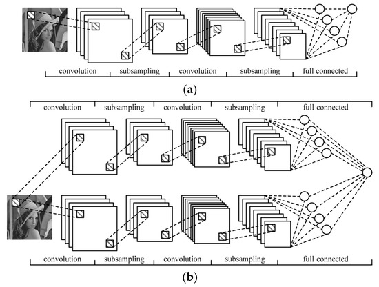
Figure 1.
Structure of convolutional neural networks (CNNs): (a) structure of a single-channel CNN; (b) structure of a multi-channel CNN.
Figure 2 shows the convolution layer of a multi-channel CNN. Convolution layers are used to extract the features from the input data by performing 3-dimensional matrix multiplication and accumulation operations between the convolution filters and the input feature maps. The computation process can be formulated as follows.
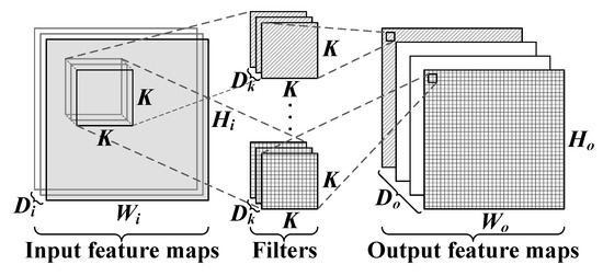
Figure 2.
Convolution layer of a multi-channel CNN.
In Equation (2), oi,j,k represents the output value of the kth output feature map at the position of (i,j). While xi+h,j+m,c represents the input value of the cth input feature map at the position of (i + h,j + m), wh,m,c,k represents the weight value of the kth filter at the position of (h,m,c), and bk represents the bias value of the kth filter. By sliding the position of the convolution filter, the convolution layer can extract all the features of the input data.
Pooling layers are usually located behind convolution layers to perform down-sampling of the extracted features, which improves the tolerance of CNNs to the distortion from input data. As shown in Figure 3, the computation process of pooling layers first divides each input feature map into a plurality of non-overlapping rectangular sub-regions; then, it performs maximum or an average operation on the pixels in each sub-region. The existence of the pooling layer effectively reduces the size of a CNNs model.
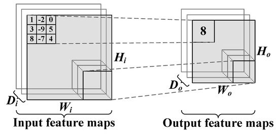
Figure 3.
Pooling layer structure.
Fully connected layers using 2-dimensional matrix multiplications to realize the fully connected mapping from Di input neuron to Do output neuron, which is similar to the convolution layer, but much simpler. The computation process can be formulated as shown in Equation (3), where oj represents the jth output neuron, Wi,j represents the weights between the ith input neuron and the jth output neuron, xi represents the ith input neuron, and bj represents the bias of the jth output neuron.
3.2. Network Traffic Preprocessing
Network traffic in cyberspace is composed of multiple Ethernet messages. As shown in Figure 4, each frame of Ethernet message includes five parts: destination address, source address, type, data, and Frame Check Sequence (FCS). The destination address is the media access control (MAC) address of the receiver. The source address is the MAC address of sender. Type is a 2-bytes component that represents the protocol used in the network layer. The data part is composed of high-level protocol, data, and filler, which has a length between 46 and 1500 bytes. FCS is a check sequence used to determine whether the data package is damaged during transmission [17]. Generally speaking, the front part of the data is usually the connection data and a small amount of message content; this should reflect the intrinsic characteristics of the traffic, as the bit streams in data contain signatures of corresponding flow. This choice is very similar with [18,19], which researched malware traffic identification with the classic machine learning approach. Malware traffic classification in this paper mainly aims at the data part of each frame in network traffic, so other information needs to be anonymized and cleared.
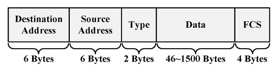
Figure 4.
Frame format of Ethernet message.
At the same time, the length of the data part is generally between 46 and 1500 bytes, which is uncertain. In order to fairly compare the ability of different CNNs for malware traffic classification, the input size should cover half the maximum length; as a result, the input data size of CNNs is limited as a 28 × 28 gray image in this paper. Thus, all of the data parts should be trimmed to the uniform length of 784. If the data size is larger than 784 bytes, it is trimmed to 784 bytes. If the data size is shorter than 784 bytes, then bytes of 0x00 will be added in the end to complement it to 784 bytes. Since only the first hundred bytes are used, this method can be much more lightweight than many others. Then, the normalized data parts with the same size are converted into gray images to generate IDX files as the training and test dataset of CNNs. The flow of network traffic preprocessing above can be divided into four steps, which are shown in Figure 5.
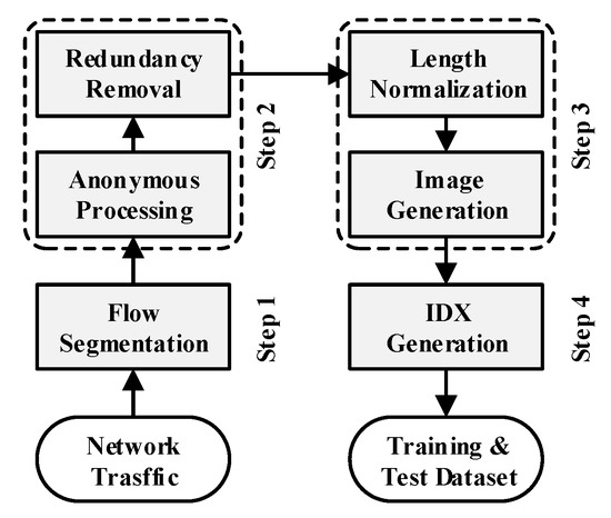
Figure 5.
Network traffic preprocessing.
In this paper, an open-source traffic dataset named USTC-TFC2016 is used to generate IDX files for training and testing the CNNs models [8]. USTC-TFC2016 consists of two parts, as shown in Table 1 and Table 2, and it includes both encrypted and unencrypted raw traffic. The size of the USTC-TFC2016 dataset is 3.71 giga bytes (GB), and the format is pcap.

Table 1.
USTC-TFC2016 malware traffic.
Table 2.
USTC-TFC2016 normal traffic.
Part I contains 10 types of malware traffic from a public website that were collected from a real network environment by a Czech Technical University (CTU) researcher from 2011 to 2015 [20]. Part II contains 10 types of normal traffic, which were collected by using IXIA BPS [21]; IXIA BPS is a kind of professional network traffic simulation equipment. The training dataset and test dataset for CNNs are obtained by preprocessing the above 20 kinds of network traffic.
The training dataset and test dataset are independent of each other and do not contain any data of each other. The training set is used as the input data of the CNNs model in the training stage, so that the CNNs model can learn the characteristics from the raw traffic data. The test set is used to obtain the classification accuracy of the trained model and evaluate its classification performance.
Figure 6a shows some gray images that are generated during network traffic preprocessing; the gray images have been reshaped to the size of 784 × 784 to provide a clearer visual experience. Due to the random selection of gray images for each kind of network traffic, an obvious difference can still be seen from Figure 6a. Therefore, Figure 6b shows several carefully selected sets of grayscale images, including Geodo, shifu, Zeus, Facetime FTP, and Weibo. There are significant differences among the three images in each group, which further indicates that it is very difficult to design proper feature sets for traditional traffic classification methods.
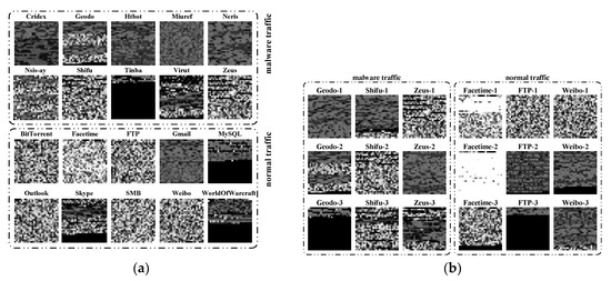
Figure 6.
(a) Random selection of gray images for each kind of network traffic; (b) Carefully selected sets of grayscale images for several kinds of network traffic.
4. CNNs-Based Malware Classification
In this section, four different CNNs are constructed and trained to classify malware traffic and normal traffic. Through experiments and comparisons, LeNet is found to be good and stable. Then, the performance of LeNet with different convolution kernel sizes is evaluated. Finally, the LeNet model is quantified to evaluate the impact of different quantization methods on test accuracy.
4.1. Architecture of CNNs
As shown in Figure 7, four different CNNs are constructed, including LeNet, AlexNet, VGGNet, and ResNET. LeNet is the first CNN designed by Yann LeCun for handwritten digit recognition in 1998; it is one of the most representative experimental CNNs in early years. AlexNet has a very similar architecture as LeNet but it is deeper, with more filters per layer; it was designed by Alex Krizhevsky and published with Ilya Sutskever and Krizhevsky’s doctoral advisor Geoffrey Hinton. VGGNet is a further improvement on the basis of AlexNet. ResNet is an artificial neural network of a kind that builds on constructs known from pyramidal cells in the cerebral cortex by utilizing skip connections or shortcuts to jump over some layers. In this paper, LeNet, AlexNet, VGGNet, and ResNet are modified slightly.
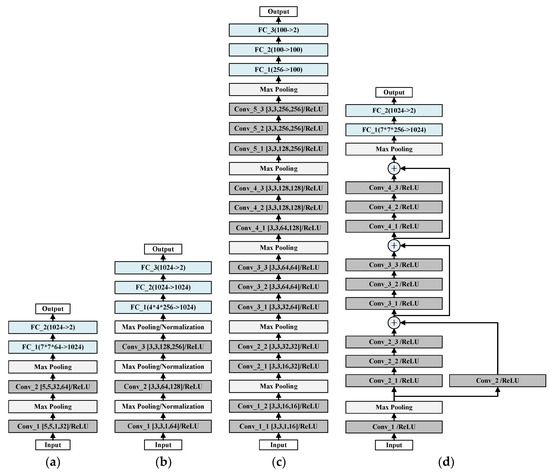
Figure 7.
Structure of four CNNs: (a) architecture of LeNet; (b) architecture of AlexNet; (c) architecture of VGGNet; (d) architecture of ResNet.
The input of each CNN is 28 × 28 two-dimensional data, and the output indicates whether the current traffic is malicious. As shown in Figure 7a, LeNet consists of two convolution layers and two fully connected layers: Conv_1, Conv_2, FC_1, and FC_2. There are 32 convolution kernels in Conv_1, and the size of each kernel is 5 × 5. Conv_2 has 64 convolution kernels, each kernel is a three-dimensional matrix, and the size is 32 × 5 × 5. AlexNet in Figure 7b includes three convolution layers and three fully connected layers, which has a very similar structure to LeNet. However, the amount of the convolution kernels in AlexNet is larger than that of LeNet. The size of each convolution kernel is specified in Figure 7b, which will not be described anymore. As shown in Figure 7c, VGGNet contains 13 convolution layers and three fully connected layers. ResNet in Figure 7d is quite different from the others; it consists of 11 convolution layers, 2 fully connected layers, and three residual layers.
4.2. Training and Testing CNNs
The training dataset generated in Section 2 is used to train the above four CNNs; then, four models for malware traffic classification are obtained. The training curves of the four CNNs are shown in Figure 8. First, 100 random images from the training dataset are used in each training step. As shown in Figure 8a, it is the training curve of LeNet; Figure 8b is the training curve of AlexNet; Figure 8c shows the training curve of VGGNet; Figure 8d is the training curve of ResNet.
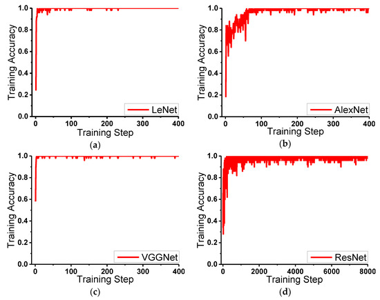
Figure 8.
Training process of four CNNs: (a) training curve of LeNet; (b) training curve of AlexNet; (c) training curve of VGGNet; (d) training curve of ResNet.
The following conclusions can be summarized from Figure 8. In terms of the training speed, LeNet and VGGNet are fast, AlexNet is normal, and ResNet is slow. In terms of training stability, LeNet and VGGNet are stable, AlexNet is normal, and ResNet is unstable. It is worth noting that ResNet uses 8000 training steps in total, while the other three CNNs only use 400 training steps, which indicates that the training process of ResNet is much slower than the others.
For further evaluation of these four CNNs, the above training process is repeated another four times. It means that 20 models can be obtained totally: five models for each kind of CNN. After that, the test dataset generated in Section 2 is used to evaluate all 20 models. As shown in Table 3, it is the test accuracy results of the above four CNNs. The calculation of test accuracy is shown in Equation (4), where TP represents the number of normal traffic correctly identified, TN is the number of malware traffic correctly identified, FP is the number of normal traffic identified as malicious, and FN represents the number of malicious traffic identified as normal. The test accuracy of the LeNet model is 99.89%, 99.92%, 99.88%, 99.87%, and 99.90% respectively; the test accuracy of the AlexNet model is 99.60%, 99.63%, 99.44%, 99.33%, and 99.60%; the accuracy of the VGGNet model is 98.99%, 99.87%, 99.93%, 99.90%, and 99.56%; and the accuracy of the ResNet model is 99.80%, 99.46%, 99.58%, 99.75%, and 99.41%. This kind of accuracy description method can not reflect the generalization performance of each CNN very accurately. As a result, the data are transformed into a curve, as shown in Figure 9.
Table 3.
Test accuracy of four convolution neural networks.
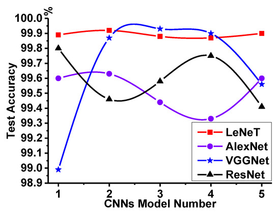
Figure 9.
Generalization performance comparison of four CNNs.
Figure 9 shows the generalization performance comparisons of four CNNs. It can be seen that the test accuracy of LeNet is smooth, which indicates that LeNet has good and stable classification ability for malware traffic and normal traffic. The test accuracy of AlexNet is slightly smaller than that of LeNet. The test accuracy VGGNet is unstable, which means that VGGNet has no strong generalization ability for malware traffic classification. Therefore, it is reasonable and practical to do malware traffic classification by using LeNet.
4.3. Different Convolution Kernel Size for LeNet
As mentioned above, the applicability of four CNNs to malicious traffic classification is analyzed. LeNet is finally determined as the most suitable CNN, which is used to classify malicious traffic in this paper. In order to further evaluate the performance of LeNet with different convolution kernels, Conv_1, Conv_2, and FC_1 of LeNet in Figure 7a are modified to different sizes, which is shown in Figure 10.
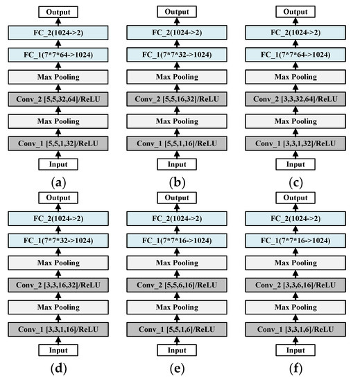
Figure 10.
Architecture of LeNet with different convolution kernels: (a) LeNet-A; (b) LeNet-B; (c) LeNet-C; (d) LeNet-D; (e) LeNet-E; (f) LeNet-F.
The original architecture is shown in Figure 10a, which is named as LeNet-A in the following sections. The architecture of LeNet-B is given as Figure 10b; the convolution kernel size of Conv_1 is [5,5,1,16], while Conv_2′s size is [5,5,16,32]. The other four architectures of LeNet are defined in Figure 10c–f. The sizes of their convolution kernels Conv_1 are [3,3,1,32], [3,3,1,16], [5,5,1,6], and [3,3,1,6]; and the sizes of Conv_2 are [3,3,32,64], [3,3,16,32], [5,5,6,16], and [3,3,6,16]. In addition, LeNet-A and LeNet-C, LeNet-B and LeNet-D, LeNet-E and LeNet-F have the same size of FC_1. The rest of the layers in the six LeNet architectures are exactly the same.
Table 4 shows the test accuracy results of the above six architectures. It can be seen from the table that the convolution kernel size has little influence on the accuracy of malicious traffic classification. A large convolution kernel size means more multiplications; it will seriously affect the inference efficiency of the LeNet model. In addition, it can be further seen that LeNet has good and stable classification ability. LeNet-F is finally chosen as the target CNN in this paper.
Table 4.
Test accuracy of six LeNet architectures.
4.4. Quantization of LeNet-F
Quantization is an important method to simplify the CNN model. With 8-bit quantization, the model size can be reduced by a factor of four, with negligible accuracy loss [22,23]. Table 5 shows the test accuracy results of the 32 bit, 16 bit, and 8 bit quantizated LeNet-F models. It can be seen that the 8-bit quantized model has almost the same test accuracy with that of the 32-bit quantized model. As a result, the 8-bit quantized LeNet-F model is used to optimize the inference efficiency in the following FPGA acceleration.
Table 5.
Test accuracy of quantized LeNet-F models.
The topology of the LeNet-F model is shown in Figure 11. There are two convolution layers, two pooling layers, and two fully connected layers. The two convolution layers are named as C1 and C2 respectively, and the size of the convolution output is 6@28 × 28 and 16@14 × 14. The two pooling layers are named as S1 and S2, and the size of the output is 6@14 × 14 and 16@7 × 7. The two fully connected layers are named as F1 and OUTPUT, and their output sizes are 1024 and 2.
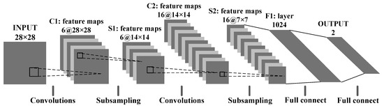
Figure 11.
Topology of the LeNet-F model.
5. Hardware Design Architecture
5.1. FPGA Acceleration Overview
Figure 12 shows an overview of the FPGA acceleration framework proposed in this paper. The acceleration framework is divided into two parts: Programmable Logic (PL) and Processing System (PS). The PL side consists of a parameterized hardware accelerator and a direct memory access (DMA) controller responsible for transferring data between external memory and on-chip buffers. The hardware accelerator is named as Compute Engine, which consists of four components: Conv-FC Engine, Pooling Engine, Control Logic, and On-Chip Memory System. The PS side is mainly composed of an ARM cortex-A9 dual-core processor, in which an Ubuntu operating system is running. A software framework is designed to interact with the underlying hardware logic and also provides a convenient user interface for the fast deployment of CNNs applications. Data transactions between PS and PL are realized by using a shared synchronous dynamic random-access memory (SDRAM).
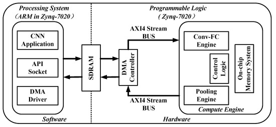
Figure 12.
Field programmable gate array (FPGA) acceleration framework for malware traffic classification.
5.2. Compute Engine
5.2.1. Conv-FC Engine
In order to make full use of dsp48e1 slice resources in FPGA, the convolution layers and the fully connected layers are implemented in the same module, which is named as Conv-FC Engine in this paper. Figure 13 shows the structure of Conv-FC Engine.
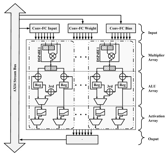
Figure 13.
Convolution acceleration module.
Conv-FC Engine consists of three parts: a multiplier array, arithmetic logic unit (ALU) array, and activation array, which are fully pipe-lined between each other. Each multiplier unit, ALU unit, and activation unit constitute two computation cells. The multiplier array is composed of 205 dsp48e1s and 205 buffers. By using the advantage of 18 × 27 bit input width, two int8 multiplication operations can be implemented in each dsp48e1 [22]. At the same time, the 205 dsp48e1s are full parallelism optimized. As a result, the multiplier array can perform up to 410 8-bit multiplication operations per clock cycle. The ALU array is responsible for accumulating the output of the multiplier unit corresponding to each output channel. This part contains a total of 205 accumulators; each one consists of three adders and two buffers. The iteration number of the accumulating units is generated by the Control Logic. The activation array is a hardware implementation of the RELU function. It consists of 205 RELU activation units; each one is simply implemented by two comparators. As fully connected layers do not use activation functions, the activation unit can be skipped under the influence of Control Logic in that case.
As mentioned above, two convolution operations named C1 and C2 are performed in LeNet-F. For C1 operation, calculations are divided into 2 × 6 batches; each batch uses 392 computation cells, and each cell is accumulated nine times, which takes about 9 × 2 × 6 clock cycles. The calculations in C2 are larger than those of C1; they are divided into 3 × 16 batches, the same 392 computation cells are used in each batch, and each cell is accumulated the same number of times as that of C1. Therefore, the whole C2 operation takes about 9 × 3 × 16 clock cycles.
Different from convolution operations, fully connected operations complete a set of calculations with two computation cells at the same time by activated the 3rd adder in the ALU unit. It means that only half of the clock cycle is needed for each calculation in the F1 and OUPUT layers. Calculations in F1 are divided into five batches; the former for batches use 410 computation cells, while the last one used 408 computation cells. Each cell is accumulated 392 times, and a total of 392 × 5 clocks were used to finish calculations in the F1 layer. The calculations in OUTPUT are smaller than those of F1, so there is no need to divide the calculations into batches. The 1024 calculations in each channel are distributed into eight computation cells, and each cell is accumulated 128 times. Finally, the 8 × 2 output results are obtained and sent to the PS side to further compute the final two-channel output.
As described in Table 6, the size of the data filled into Conv-FC Input is determined by ALU × Bat; the data size required by Conv-FC Weight is determined by ALU × (TN × [R]); 1 × TN × [R] determines the data size to be filled into Conv-FC Bias at the same time, and the size of the data output to Conv-FC Output depends on Bat. In the previous descriptions, ALU represents the number of accumulation operations, which also means the depth of data storage space for Conv-FC Input and Conv-FC Weight; the number of computation cells used in each batch is represented by Bat, which is equal to the number of the used storage units. Meanwhile, TN × [R] represents the number of the used storage units for Conv-FC Weight and Conv-FC Bias, TN represents the number of parameters, and [R] is the number of times the parameters need to be copied. In general, the data in Table 6 provide the basis for the design of the on-chip memory system.
Table 6.
Data requirement of each operation.
5.2.2. Pooling Engine
Pooling Engine has a similar computation structure to Conv-FC Engine, which is shown in Figure 14. It can be seen from Figure 11 that the pooling layers are closely connected with the convolution layers. Since the batch size for the C1 and C2 layer is 392, a total of 392 pooling cells are constructed in Pooling Engine. Each pooling cell consists of three comparators and two buffers. As the batch size of convolution and pooling are the same, the pooling operation can be started whenever the convolution batch completes the calculation. Convolution and pooling can be performed in parallel without affecting each other, which can effectively improve the computation efficiency.
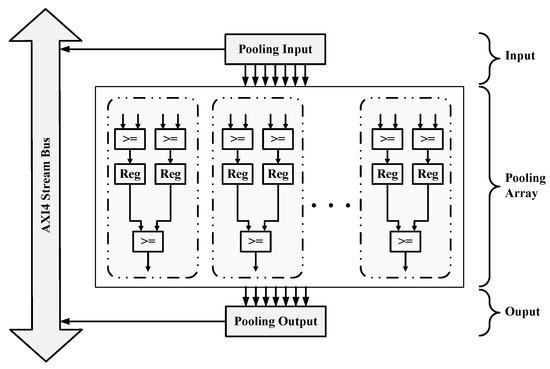
Figure 14.
Pooling acceleration module.
5.2.3. On-Chip Memory System
Multiple parameters and input data need to be acquired by the above acceleration engines at the same time when they are running at full speed. According to the system structure of the FPGA accelerator, there are six groups of data to be stored, including Conv-FC Input, Conv-FC Weight, Conv-FC Bias, Conv-FC Output, Pooling Input, and Pooling Output. It is hard to meet the data requirements of the acceleration modules by purely using an external memory interface to feed the Compute Engine with data. To solve this problem, an on-chip memory system is designed to transfer all the parameters and in–out data into the accelerator through an AXI4 stream bus in burst mode, which is shown in Figure 15.
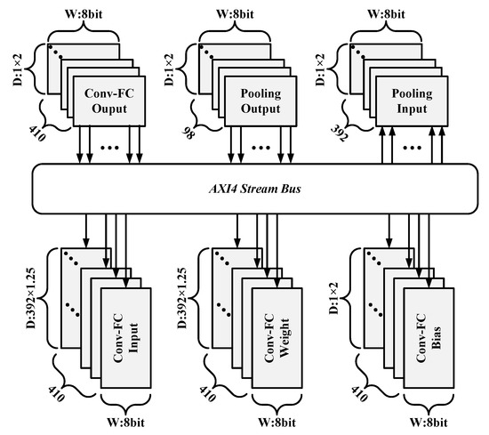
Figure 15.
On-chip Memory System.
All the storage units mentioned above are implemented with First Input First Output (FIFO). It can be analyzed from Table 6 that 410 FIFOs are required for both Conv-FC Input and Conv-FC Weight, and the depth of each FIFO is not less than 392. Conv-FC Bias and Conv-FC Output also require 410 FIFOs, but the depth only needs to be greater than or equal to 1. As mentioned in the previous section, the size of Pooling Input is 392, which means it requires 392 FIFOs, and the depth of each FIFO is at least 1; the storage depth of Pooling Output is the same as that of Pooling Input, but only 98 FIFOs are used. In order to make more efficient use of FIFO, this paper reserved extra depth for all the storage units in the on-chip memory system, which saves the time waiting for data reading and writing, and it improves the data processing efficiency of the acceleration system.
5.2.4. Runtime Reconfigurabilty
In order to realize real-time reconfigurability, parameters must be transferred into a global register list before the calculation of each engine. The transmission of configuration parameters usually has two options: a dedicated control bus or data format agreed in advance via data bus. In this paper, the latter method is selected because it does not require additional hardware resources and is easier to control compared to the former.
Figure 16 shows the data format of the input stream in our design. The accelerator buffers the first eight words in a burst transmission as configuration parameters into the global register list in Control Logic. The first byte named as Function Mode is streamed into Control Logic, which indicates the type of the current computation, and the corresponding acceleration engine will be started by Control Logic. Then, the started acceleration engine continues decoding the rest of the parameters in the register list and generating control signals for the whole computing process. However, the decoding results of each engine are not same, as shown in Table 7. When Function Mode = 0, Control Logic enables Conv-FC Engine, and the second byte called ALU Mode indicates whether the 3rd adder in Conv-FC Engine is activated. ALU Repeat, Batch Size, Weight Size, Bias Size, and Parameter Copy correspond to the parameters in Table 6. When C1, C2, F1, and OUTPUT operations are executed, different parameters are needed to complete the corresponding calculations.
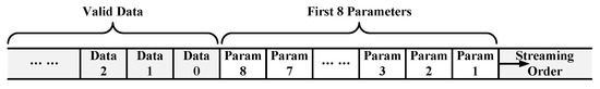
Figure 16.
Format of input data stream.
Table 7.
Decoding results of each acceleration module.
5.3. Software Framework
For the fast deployment of CNNs models, a three-layer software framework is designed, which is based on the PYNQ open source framework. PYNQ is an open-source project from Xilinx that makes it easy to design embedded systems with Xilinx-Zynq systems on chips. The CNNs mapping flow based on our framework is shown in Figure 17. Python classes in the driver layer are mainly responsible for managing the underlying hardware accelerator and programming the bitstream file into FPGA. The Application Program Interface (API) layer provides a friendly user interface by encapsulating the classes of the driver layer; users can call the interface in the API layer to quickly build a CNN acceleration by mapping the model into FPGA. The application layer contains a parameter parser for extracting the structure parameters and weight parameters of the given pre-trained model, and a model constructor that calls the API layer classes to build a FPGA-based CNNs model automatically. Figure 18 shows an example of LeNet-F model-3; it is constructed by using the API layer interface above, corresponding to the model architecture given in Section 4. It can be seen that the CNNs acceleration based on this software framework is very simple, clear, and easy to be deployed quickly.
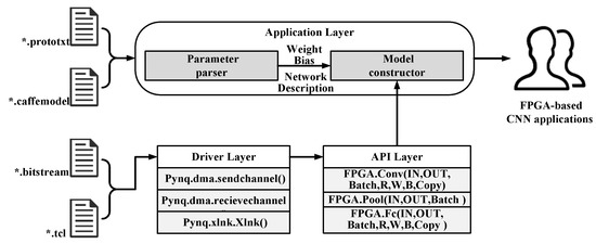
Figure 17.
Software framework and mapping flow.
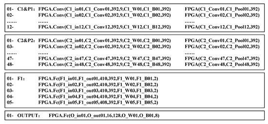
Figure 18.
LeNet-F model-3 constructed by using an API interface.
6. Typical Application and Experimental Results
6.1. Experiment Setup
As shown in Figure 19, a typical application of an FPGA accelerator for CNNs-based malware traffic classification is constructed in this paper. The whole system above is evaluated on an MZ7XB evaluation board, which is shown in Figure 20. This board features a Xilinx XC7Z020-clg400 chip that integrates an ARM cortex-A9 dual-core CPU working at a clock frequency of 650 MHz, two gigabit network interfaces on the PL side and one gigabit network interface on the PS side. The sender and the receiver are connected to the two gigabit network interfaces on the PL side, and they are both able to transfer their own network traffic in two directions. An Ubuntu operating system is running on the ARM CPU, which can be accessed via the gigabit interface of the PS side.
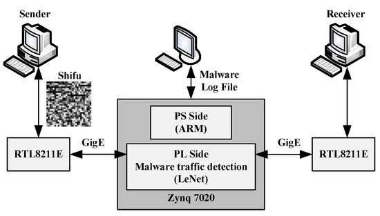
Figure 19.
Typical application system of the FPGA accelerator for CNN-based malware traffic classification.
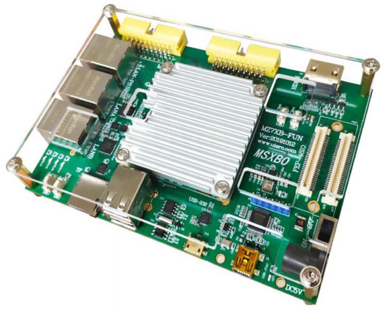
Figure 20.
Zynq-7020 evaluation board.
The LeNet-F model-3 is finally chosen as the CNN model to validate the performance of the proposed FPGA accelerator for CNN-based malware traffic classification in this paper. The parameters of the pre-trained LeNet-F model-3 are extracted and quantified, and they are deployed into the FPGA accelerator for a performance test. Then, 10,000 frames of traffic are transmitted from the sender to the receiver, all the classification results are stored in the PS side. If any frame of traffic is malicious, it will not be transmitted to the receiver, but it will be logged in the file. As a result, the test accuracy of the system can be calculated from the number of the malware traffic frames.
6.2. Results Analysis
Table 8 shows the resource utilization of the target FPGA. BRAMs, DSPs, FFs, and LUTs mean the amount of block rams, digital signal processors, flip-flops, and lookup tables used in the proposed accelerator. Since our design fully explores the parallelism of CNNs and the 8-bit int format is used for calculation, 205 DSPs are used. Up to 210 BRAMs are used due to the optimization of the on-chip memory system. However, it can be seen from Table 8 that the on-chip resources are not fully utilized, which provides an improvement space of acceleration performance for future works.
Table 8.
Resource utilization of the field programmable gate array (FPGA) accelerator.
Table 9 shows the results of LeNet-F model-3 implementations on other different platforms, including Intel Xeon E5-2680, F-CNN [24], and the graphic process unit (GPU) platform of NVIDIA Tesla K20X; six groups of data are listed. The consumption of LUTs is 31,201 in the proposed accelerator and 68,510 in F-CNN, which is reduced by 54.46%. The usage of BRAMs is 210, which is 510 in FCNN: a reduction of 58.82%. The amount of DSPs used in our design is 205, which is far more than 23 in F-CNN, but the identification for a single frame of our FPGA accelerator is much faster. As shown in Table 9, the identification of a single traffic packet only needs 18.97 μs, which is 42.2 times faster than the 804.33 μs under the Intel Xeon E5-2680 platform, and the speed increased by 6.2 times compared to 117.67 μs on F-CNN, which is also 7.04 times faster than 133.5 μs under the GPU platform. Comparing with the implementation based on Intel Xeon E5-2680 and NVIDIA Tesla K20x, this paper loses only 0.01% recognition accuracy from 99.78% to 99.77%. F-CNN is tested with MINST data set; thus, the test accuracy is not comparable with our design. Assume that the average size of each traffic packet is 1 kilo bytes (KB); then, the throughput of the system above can reach 411.83 Mbps, which is calculated as shown in Equation (5).
Table 9.
Performance comparison of different works.
7. Conclusions
In this paper, four CNNs are used to classify malware traffic and normal traffic. Through experiments and comparisons, it is found that LeNet has good and stable classification ability for malware traffic and normal traffic. There is no need to hand-design the traffic feature sets beforehand. The raw traffic data are the direct input data of the traffic classifier, and the classifier can learn features automatically.
Meanwhile, an FPGA accelerator for CNN-based malware traffic classification is designed. As a result, the CNN accelerator implemented on FPGA loses only 0.01% of classification accuracy from 99.78% to 99.77%. It can classify each traffic image from the training and test dataset in 18.97 μs under the clock frequency of 150 MHz, which is 6.2 times faster than F-CNN, 42.2 times faster than Intel Xeon E5-2680, and 7.04 times faster than NVIDIA Tesla K20X. The implementation keeps the balance between resource occupancy and computation speed, which makes it possible to deploy CNN-based malware traffic classification in portable devices. The throughput of the typical application system designed in this paper can reach 411.83 Mbps.
Through the research and application in this paper, we can quickly train a CNN model for malware traffic classification from the raw traffic within a couple of hours in the actual application scenario, which can effectively resist malware traffic attacks from hackers to a large extent. By integrating a hardware accelerator for CNN-based malware traffic classification in portable devices, not only can the CPU resources be released and the energy consumption reduced, but secure and real-time data transmission can be effectively guaranteed as well.
In the future, in order to further improve the bandwidth to meet the communication requirements of the gigabit network, a multi-core parallel acceleration scheme can be adopted. In addition, four int4 multiplication operations can be implemented in each dsp48e1; therefore, the model can be further quantified to implement more calculations in each clock cycle. Thirdly, in order to meet the requirements of low power consumption and light weight in portable devices, LeNet was chosen to be implemented on FPGA for the hardware acceleration of malware traffic classification. However, other CNNs can also be applied on the FPGA acceleration platform in this paper, which can explore the feasibility of hardware acceleration for other anomaly detections later. At the same time, BNN is also very attractive. These research directions will be further carried out in the future.
Author Contributions
Conceptualization, L.Z.; methodology, L.Z. and Y.L.; software, L.Z.; validation, L.Z.; formal analysis, L.Z.; resources, L.Z.; writing—original draft L.Z.; writing—review and editing, B.L., Y.L., X.Z., Y.W. and J.W.; supervision, B.L. All authors have read and agreed to the published version of the manuscript.
Funding
This work was supported by the ShenZhen Science Technology and Innovation Commission (SZSTI): JCYJ20170817115500476 & JCYJ20170817115538543.
Conflicts of Interest
The authors declare no conflict of interest.
References
- Biersack, E.; Callegari, C.; Matijasevic, M. Data Traffic Monitoring and Analysis; Springer: Berlin/Heidelberg, Germany, 2013. [Google Scholar]
- Rathore, H.; Agarwal, S.; Sahay, S.K.; Sewak, M. Malware Detection Using Machine Learning and Deep Learning. Big Data Analytics; Springer: Berlin/Heidelberg, Germany, 2018. [Google Scholar]
- Dhote, Y.; Agrawal, S.; Deen, A.J. A Survey on Feature Selection Techniques for Internet Traffic Classification. In Proceedings of the International Conference on Computational Intelligence and Communication Networks (CICN), Jabalpur, India, 12–14 December 2015; pp. 1375–1380. [Google Scholar]
- Bengio, Y.; Courville, A.; Vincent, P. Representation learning: A review and new perspectives. IEEE Trans. Pattern Anal. Mach. Intell. 2013, 35, 1798–1828. [Google Scholar] [CrossRef] [PubMed]
- LeCun, Y.; Bengio, Y.; Hinton, G. Deep learning. Nature 2015, 521, 436–444. [Google Scholar] [CrossRef] [PubMed]
- Qingqing, Z.; Yong, L.; Zhichao, W.; Jielin, P.; Yonghong, Y. The application of convolutional neural network in speech recognition. Microcomput. Appl. 2014, 3, 39–42. [Google Scholar]
- Hinton, G.E.; Salakhutdinov, R. Reducing the dimensionality of data with neural networks. Science 2006, 313, 504–507. [Google Scholar] [CrossRef] [PubMed]
- Wang, W.; Zeng, X.; Ye, X.; Sheng, Y.; Zhu, M. Malware Traffic Classification Using Convolutional Neural Networks for Representation Learning. In Proceedings of the 31st International Conference on Information Networking (ICOIN 2017), Da Nang, Vietnam, 11–13 January 2017; pp. 712–717. [Google Scholar]
- Gu, J.; Wang, Z.; Kuen, J.; Ma, L.; Shahroudy, A.; Shuai, B.; Liu, T.; Wang, X.; Wang, G.; Cai, J.; et al. Recent advances in convolutional neural networks. Pattern Recognit. 2018, 77, 354–377. [Google Scholar] [CrossRef]
- Dreger, H.; Feldmann, A.; Mai, M.; Paxson, V.; Sommer, R.R. Dynamic Application Layer Protocol Analysis for Network Intrusion Detection. In Proceedings of the 15th USENIX Security Symposium, Vancouver, BC, Canada, 31 July–4 August 2006. [Google Scholar]
- Finsterbusch, M.; Richter, C.; Rocha, E.; Muller, J.-A.; Hanssgen, K. A survey of payload-based traffic classification approaches. IEEE Commun. Surv. Tutor. 2014, 16, 1135–1156. [Google Scholar] [CrossRef]
- Gao, N.; Gao, L.; Gao, Q. An Intrusion Detection Model Based on Deep Belief Networks. In Proceedings of the Second International Conference on Advanced Cloud and Big Data, Huangshan, China, 20–22 November 2014; pp. 247–252. [Google Scholar]
- Javaid, A.; Niyaz, Q.; Sun, W.; Alam, M. A Deep Learning Approach for Network Intrusion Detection System. In Proceedings of the 9th EAI International Conference on Bio-inspired Information and Communications Technologies, New York, NY, USA, 3–5 December 2015. [Google Scholar]
- Tavallaee, M.; Bagheri, E.; Lu, W.; Ghorbani, A.A. A Detailed Analysis of the KDD CUP 99 Data Set. In Proceedings of the IEEE Symposium on Computational Intelligence in Security and Defense Applications, Ottawa, ON, Canada, 8–10 July 2009; pp. 53–58. [Google Scholar]
- Wang, Z. The Applications of Deep Learning on Traffic Identification. Available online: https://goo.gl/WouIM6 (accessed on 1 October 2020).
- Zhang, L.; Bu, X.; Li, B. XNORCONV: CNNs accelerator implemented on FPGA using a hybrid CNNs structure and an inter-layer pipeline method. IET Image Process. 2020, 14, 105–113. [Google Scholar] [CrossRef]
- Heywood, D.; Ahmad, Z. Drew Heywood’s Windows 2000 Network Services; Sams: Carmel, IN, USA, 2001. [Google Scholar]
- Celik, Z.B.; Walls, R.J.; McDaniel, P.; Swami, A. Malware traffic detection using tamper resistant features. In Proceedings of the Military Communications Conference, MILCOM 2015–2015, Tampa, FL, USA, 26–28 October 2015; pp. 330–335. [Google Scholar]
- Li, W.; Canini, M.; Moore, A.W.; Bolla, R. Efficient application identification and the temporal and spatial stability of classification schema. Comput. Netw. 2009, 53, 790–809. [Google Scholar] [CrossRef]
- CTU University. The Stratosphere IPS Project Dataset. Available online: https://strato-sphereips.org/category/dataset.html (accessed on 1 October 2020).
- Ixia Corporation. Ixia Breakpoint Overview and Specifications. Available online: https://www.ixiacom.com/products/breakingpoint (accessed on 1 October 2020).
- Dettmers, T. 8-Bit Approximations for parallelism in deep learning. arXiv 2015, arXiv:1511.04561. [Google Scholar]
- Han, S.; Mao, H.; Dally, W.J. Deep compression: Compressing deep neural networks with pruning, trained quantization and huffman coding. arXiv 2016, arXiv:1510.00149. [Google Scholar]
- Zhao, W.; Fu, H.; Luk, W.; Yu, T.; Wang, S.; Feng, B.; Ma, Y.; Yang, G. F-CNN: An FPGA-based Framework for training Convolutional Neural Networks. In Proceedings of the 27th International Conference on Application-Specific Systems, Architectures and Processors (ASAP), London, UK, 6–8 July 2016; pp. 107–114. [Google Scholar]
© 2020 by the authors. Licensee MDPI, Basel, Switzerland. This article is an open access article distributed under the terms and conditions of the Creative Commons Attribution (CC BY) license (http://creativecommons.org/licenses/by/4.0/).