A Novel Calibration Method for Signal Leakage between Multiple Channels in Array Imaging

Abstract

In this paper, the array imaging process with the presence of signal leakage between channels is derived and analyzed in short-range imaging applications. The echo wave of the system can be divided into two parts: the echo signals we expected, and the echo signal that resulted from the leaked signals. Signals leaked to the adjacent channels can lead to ghosts which can deeply deteriorate the system cross resolution. To solve this problem, a concise calibration method is proposed to remove the impacts of the signal leakages on the imaging quality. Furthermore, the results based on the simulation and the real-world data validate the effectiveness of the proposed method, which indicates that this calibration method can mostly cancel the influence of the signal leakages.

1. Introduction

Nowadays, near-field millimeter-wave imaging has been widely applied to various fields such as human body security [1,2,3,4,5,6,7], 3-D body size measurement [8,9,10], and skin cancer detection [11,12,13]. However, there are always some hardware defects in the system which can deeply deteriorate the system’s performance, especially in array imaging. Therefore, to get a high-quality image of these radar systems, some calibration processes must be done before imaging. A variety of calibration methods for different system problems have been proposed in the past, such as computational correction algorithm for nonlinearities [14,15,16], phase error correction [17,18,19], and channel imbalance correction [20,21].

Signal leakage is an important problem which needs to be processed in a radar system. Signal leakage that occurs between transmitter and receiver can cause a strong degradation of the detection sensitivity as a result of the phase noise of the transmit oscillator. Its calibration method has been widely discussed. There are several ways to deal with this leakage. One way is to increase the distance between the Tx and the Rx to reduce the leakage [22]. The second way is to add a closed loop leakage canceller which can generate an error vector including leakage amplitude and phase information, and this information can be used to carry out the calibration [23,24,25].

Signal leakage between different channels in multichannel systems is a unique problem, especially in imaging systems with requirements of high resolution and sensitivity. The leakage that occurs between the transmitter and the receiver has been widely studied. There are a lot of discussions about its signal model and processing method [26,27,28]. However the impact of the leakage that occurs between transmitters or receivers has rarely been discussed. In this paper, the array imaging process with the presence of signal leakage caused by the lower isolation between transmitters or receivers is researched. First, a common array structure and its signal leakage model between different channels are introduced. Second, the imaging process with the presence of signal leakage is derived based on the model and the influence of the signal leakage is discussed. Signals leaked to adjacent channels can lead to ghosts which can deeply deteriorate the system cross resolution. To eliminate the bad influence of the signal leakages, a calibration method operating in the beam domain is proposed next. Finally, to validate the effectiveness of the proposed method, a simulation and some experiments are carried out. All the derivation and analysis are based on a common array structure applied in short range imaging.

The paper is structured as follows. Section 2 introduces the used array structure and signal leakage model between different channels. The impacts of the channel signal leakages are analyzed in Section 3. Based on the analysis, a calibration method is prosed in Section 4. Finally, in Section 5, we verify the calibration method with a simulation and some experiments.

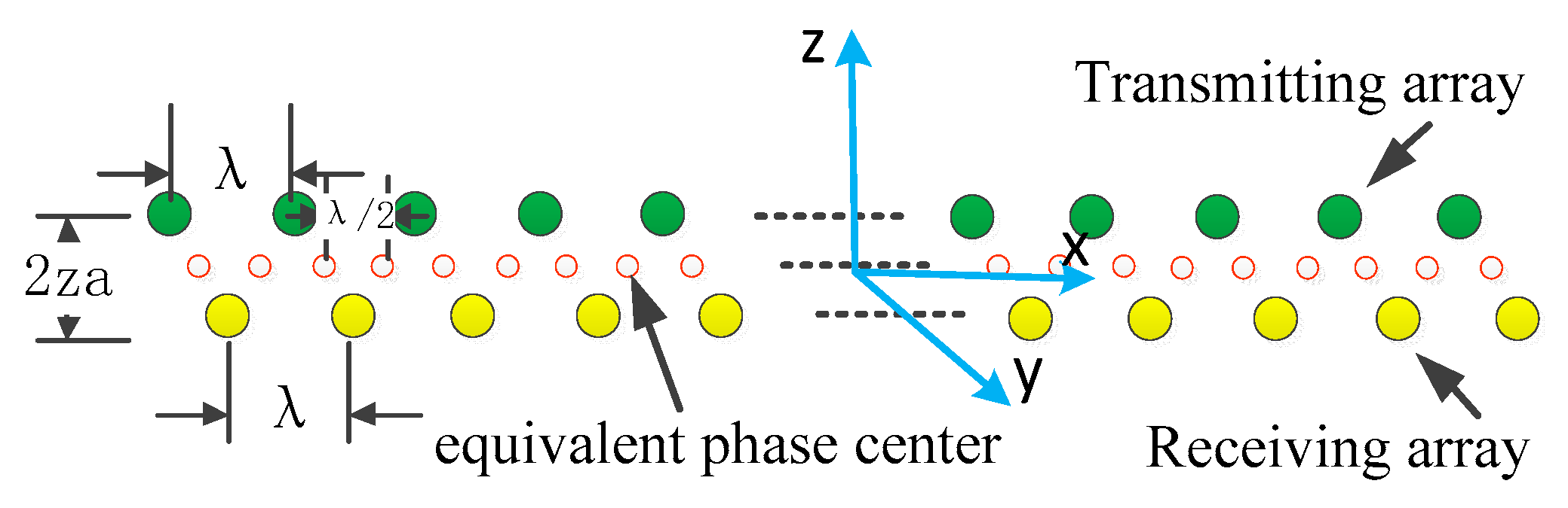
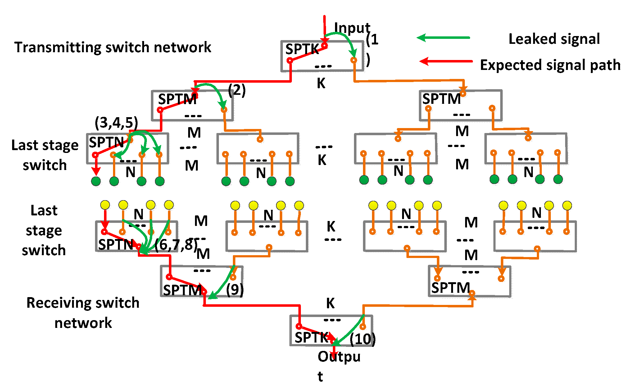
2. Array Structure and Signal Leakage Model

Figure 1 is a common antenna array structure of the millimeter wave in short range imaging [29]. The architecture of the array consists of two linear arrays. Suppose that the transmitting array is on the above and the receiving array is on the below. The interval between the transmitting or receiving elements is λ. In order to get equivalent phase centers with an interval of λ/2, the receiving array is shifted λ/2 along the x direction with respect to the transmitting array. When one transmitting element is working, its two adjacent receiving elements carry out the signal reception in sequence. The signal is usually regarded as though it is transmitted and received both at the midpoint of the line connecting the corresponding working antennas. Thus, a set of equivalent phase centers spaced λ/2 can be obtained.

In order to implement the signal’s independent emission and reception of the array units described in Figure 1, the imaging system usually adopts a multistage switch matrix. Figure 2 is a common switch network structure. For the convenience of description, a three-stage switch matrix is used in Figure 2. The first, second, and third stage of the transmitting network adopt SPTK, SPTM, and SPTN switch chips, respectively, as shown in Figure 2. The structure of the receiving switch network is the same as the transmitting. Therefore, this architecture can implement a 1 × K × M × N switch network.

Based on the structure, we can make a simple analysis about the signal leakages occurred in the switch network due to the lower isolation of the switch chips when the signal is transmitted and received. Suppose that the red path in Figure 2 is the signal path we expected; therefore, the corresponding switch channels are opening while the other channels on the same chip are closed at the same time. As the isolation of the switch is limited, some signals are leaked to the closed channels, indicated by the green lines in Figure 2. The signal leakages occur in every switch stage, but those which do not occur at the last stage do not need to be considered because they have been attenuated at least twice when they arrive at the antenna and their impacts to the imaging result are not significant. Thus, only the signal leakages that occurred at the same switch chip with the opened channel at the last stage need to be considered. That means only the N − 1 channels’ signal leakages need to be considered on the transmitting switch array or the receiving array at a certain moment.

Because the signal leaked by the transmitting array and the receiving array in the received signal at a certain time is linearly superimposed, the analysis method in this paper, such as Fourier transform, has linear properties. Therefore, in order to simplify the analysis, we can independently analyze the signal leakage’s influence of the transmitting array and the receiving array. Because the two analysis processes are similar, only the signal leakage of the transmitting array is considered, and an assumption is made that signal leakage does not exist between the receiving switch matrixes. Under this assumption, for the signal transmitted from the expected transmitting antenna and the signals leaked from the adjacent antenna, there are two sets of paths to the receiving antenna, as Figure 3 shows. In one set of paths (indicated by green and red lines in Figure 3), the signals illuminate the targets and then are reflected to the receiving antenna. In the other set of paths (indicated by yellow line in Figure 3), the signal is directly leaked to the receiving antenna without the reflection of the targets, which could be called the Tx/Rx coupling interference. The Tx/Rx coupling interference has a huge impact on the imaging quality. It usually has a higher power level compared to the target echo wave such that the phase noise occurred with it sometimes may raise up the system noise floor. It will deteriorate the dynamic range of the imaging system. However, the noise could be cancelled mostly by using the empty background noise. As such, the Tx/Rx coupling interference would not be concerned in this paper. Only the signals (original signal or the leaked signals) reflected by the targets are concerned.

Suppose that the nth transmitting element’s position is (x_n^Tx, 0, z_a) where nϵ{1, 2, …, K × M × N}. The mth receiving element’s position is (x_m^Rx, 0, −z_a) where mϵ{1, 2, …, K × M × N}. The target position is (x, y, 0). The flight trip from the nth transmitting element to the target is:

$$R^T{}_n=\sqrt{{(x-x_n{}^{Tx})}^2+y^2+z_a{}^2}$$

and from the target to the mth, the receiving element is:

$$R^R{}_m=\sqrt{{(x_m{}^{Rx}-x)}^2+y^2+z_a{}^2}$$

Then, the echo wave when the nth transmitting element and the mth receiving antenna is working can be expressed as:

$$s_{if}(k,m,n)=\sigma \exp (jk(R^T{}_n+R^R{}_m))+\eta {\displaystyle \sum _{i\in {\mathsf{\Phi }}_{(n)}}\sigma \exp (jk(R^T{}_i+R^R{}_m))}$$

(1)

where:

$${\mathsf{\Phi }}_{(n)}=\{\begin{array}{c}([\frac{n}{N}]-1)\cdot N+1:[\frac{n}{N}]\cdot N if rem(n,N)=0\\ [\frac{n}{N}]\cdot N+1: ([\frac{n}{N}]+1)\cdot N if rem(n,N)\ne 0\end{array}$$

which represents the transmitting element’ position set of the leaked signals. [A] represents the nearest integer less than or equal to A. Rem(n,N) represents the remainder after division of n by N. λ is the wavelength. k is the wavenumber 2π/λ. η is the attenuation coefficient of the leaked signal compared to the original signal (suppose that the original signal amplitude is 1). σ is the radar scattering coefficient (RCS) of the target. The echo wave consists of two parts. The first term represents the echo signal we expected, and the second term represents the echo signals that result from the leaked signals.

It is difficult to make a fast imaging calculation according to Equation (1). If the distance between the transmitting element and the receiving element is very close, then some phase center approximation can be made according to the monostatic measurement method developed by Kell [30] and we can approximate that the signal is transmitted and received at the same place at the equivalent phase center located at the midpoint of the transmitting and receiving antenna connection. The echo wave can be expressed as:

$$\begin{array}{l}{s}_{if}(k,m,n)\\ =\sigma \exp (-j2k\sqrt{{(x_t-(x_n{}^{Tx}+x_m{}^{Rx})/2)}^2+y_t{}^2})+\eta {\displaystyle \sum _{i\in \mathsf{\Phi }}\sigma \exp (-j2k\sqrt{{(x_t-(x_i{}^{Tx}+x_m{}^{Rx})/2)}^2+y_t{}^2}})\end{array}$$

(2)

According to Equation (1), the elements of the set Φ are integers in the range of n − N + 1 to n + N − 1 according to the configuration of the array described earlier. However, there are only N − 1 elements in the set Φ, not 2N − 1. As such, the Φ’s elements cannot traverse all of these numbers from n − N + 1 to n + N − 1 at a specific transmitting and receiving position. Its elements change with the transmitting element’s position. Therefore, the second term of echo Equation (2) varies with the transmitting element position. It is difficult to make a direct and clear analysis by using it. The first term can be regarded as a special case of the second term when I = n and η = 1, so we can merge the first and the second items. Based on the above reasons, we rewrite the echo wave Expression (2) as follows:

$$s_{if}(k,m,n)={\displaystyle \sum _{i=n-N+1}^{i=n+N-1}{u}_i(n)\cdot {\eta }_i\cdot } \sigma \cdot \exp ( -j2k\sqrt{{(x_t-(x_i{}^{Tx}+x_m{}^{Rx})/2)}^2+y_t{}^2})$$

(3)

where

$$u_i(n)=\{\begin{array}{c}1 \\ 0 \end{array}\begin{array}{c}if i\in \mathsf{\Phi } or i=n\\ other\end{array} \mathrm{and} {\eta }_i=\{\begin{array}{c}\eta \\ 1\\ 0\end{array}\begin{array}{c} if i\in \mathsf{\Phi } \\ if i=n\\ other\end{array}$$

Set that (x_n^Tx + x_m^Rx)/2 = x_a, considering that the transmitting interval is λ according to the system model shown in Figure 1, then we can get (x_i^Tx + x_m^Rx)/2 = (x_{i – n + n}^Tx + x_m^Rx)/2 = x_a + λ/2(i − n). Using this relation, the echo Expression (3) can be rewritten to:

$$s_{if}(k,x_a)={\displaystyle \sum _{i=n-N+1}^{i=n+N-1}{u}_i(n)\cdot {\eta }_i\cdot \sigma }\cdot \exp (-j2k\sqrt{{(x_t+(i-n)\cdot \lambda /2-x_a)}^2+y_t{}^2})$$

(4)

In this section, a common array structure applied in short range imaging is introduced. Its signal model with the presence of signal leakage is constructed as Expression (4). Based on the expression, we can do further analysis about the impacts of the signal leakage on array imaging.

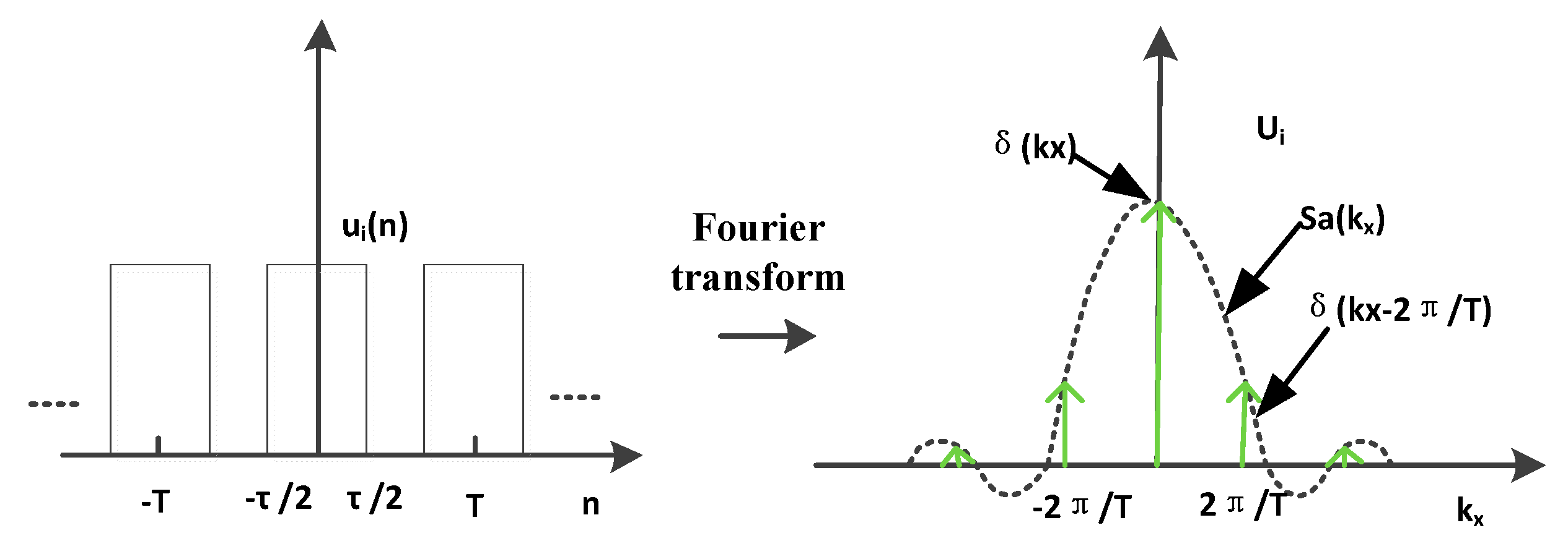
3. The Analysis of the Signal Leakage Impact on Array Imaging

Image reconstruction can be made based on Expression (4). Firstly, one-dimensional Fourier transform is implemented along the variable x_a. η_i and σ would not change with n, so we can obtain the wavenumber distribution of the echo data as follows:

$$s_{if}(k,k_x)={\displaystyle \sum _{i=n-N+1}^{i=n+N-1}{U}_i}\cdot \underset{A}{\underbrace{[{\eta }_i\cdot \sigma \exp (-j{k}_x(x_t+(i-n)\cdot \lambda /2)-j(\sqrt{4k^2-k_x{}^2})y_t)]}}$$

(5)

U_i is the Fourier transform of u_i(n). When i = n, u_n = 1, u_i(n) is a constant, its spectrum is a δ-function. When i ≠ n, u_i(n) is a periodic rectangular pulse function of receiving number n due to the special switch matrix configuration of the array and its value is between 0 and 1. Its spectrum U_i is shown in Figure 4, which can be expressed as:

$$U_i={\displaystyle \sum _{j}Sa(j\pi \tau /T)\delta (k_x-2j\pi /T)}$$

where j = 0, ±1, ±2, …, Sa(x) = sin(x)/x, τ is the pulse width of u_i(n), T is the period of the u_i(n). U_i can be seen as some δ-function combination with the envelope of Sa(jπτ/T).

We can see in Figure 4 that the power of other δ-function (δ(k_x − Δk_j), Δk_j ≠ 0) is weaker compared to the δ(k_x) because the value of Sa(k_x) decreases sharply as k_x increases. It would not have an important influence on the image. δ-functions (δ(k_x − Δk_j), Δk_j ≠ 0) will be ignored in the following derivation, namely U_i ≈ δ(k_x). γ_i is the ratio of the amplitude of δ(k_x) in U_i to the δ(k_x) in U_n. Obviously, γ_n = 1. The convolution result of δ(k_x − Δk_j) with A(k_x) is still A(k_x − Δk_j). Then, the wavenumber distribution (5) can be simplified as follows:

$$s_{if}(k,k_x)\approx {\displaystyle \sum _{i=n-N+1}^{i=n+N-1}{\gamma }_i\cdot {\eta }_i\cdot \sigma \exp (}-j{k}_x(x_t+(i-n)\cdot \lambda /2)-j(\sqrt{4k^2-k_x{}^2})y_t)$$

(6)

Set $k_y=\sqrt{4k^2-k_x{}^2}$, Expression (6) can be simplified as:

$${\mathrm{s}}_{if}(k_y,k_x)\approx {\displaystyle \sum _{i=\mathrm{n}-\mathrm{N}+1}^{i=n+N-1}{\gamma }_i\cdot {\eta }_i\cdot \sigma }\cdot \exp ( -j{k}_x(x_t+(i-n)\cdot \lambda /2)-j{k}_y{y}_t)$$

(7)

It is easy to find that the phase of S_if(k_y,k_x) is a linear combination of variable k_x and k_y. Thus, applying a 2D-FFT or 2D-IFFT on it, the image result will be obtained. One thing to notice is that the map from k to k_y is not a linear process, therefore, the k_y directly achieved form the uniformly sampled k is not equally spaced. Before the 2D-IFFT, a process called Stolt interpolation [31,32] needs to be carried out which will not be discussed in this paper. Suppose that the band of the k_x and k_y is B_x and B_y, respectively. Then, the final image result is obtained as follows after 2D-IFFT:

$$P_{original}(x,y)\approx {\displaystyle \sum _{i=n-N+1}^{i=n+N-1}{\gamma }_i\cdot {\eta }_i}\cdot \frac{2\sin (\frac{B_x}{2}\cdot (x-(x_t+(i-n)\cdot \lambda /2)))}{x-(x_t+(i-n)\cdot \lambda /2)}\cdot \frac{2\sin (\frac{B_y}{2}\cdot (y-y_t))}{y-y_t}$$

(8)

Set that

$$P(x,y)\approx \frac{2\sin (\frac{B_x}{2}\cdot (x-x_t))}{x-(x_t+(i-n)\cdot \lambda /2)}\cdot \frac{2\sin (\frac{B_y}{2}\cdot (y-y_t))}{y-y_t}$$

(9)

which can be seen as the ideal point spread function of the system. The P_original(x,y) can be rewritten as:

$$P_{original}(x,y)\approx {\displaystyle \sum _{i=n-N+1}^{i=n+N-1}{\gamma }_i}\cdot {\eta }_i\cdot P(x-(i-n)\cdot \lambda /2,y)$$

(10)

It is obvious that the original point spread function P_original(x,y) influenced by the leaked signals is a combination of the P(x,y) shifted (i − n)λ/2 in the x direction. This can deteriorate the system cross resolution. It is easy to imagine that the superposition of several pulses is usually wider than a single pulse. The larger the coefficient γ_i, the more serious the deterioration of the cross resolution is. On the contrary, the leaked signals have little impact on the range resolution according to the P_original(x,y) expression.

In this section, the imaging process is derived. The final imaging result is conveyed as Expression (10). The influence of the signal leakage proposed above is analyzed. It can deteriorate the system cross resolution but have little impact on the range resolution.

4. Calibration Method of the Signal Leakage

To eliminate the bad influences of the signal leakages, a calibration method will be proposed next. The shift in the time domain can be compensated in the frequency domain. Doing 1-D FFT along the x direction on both side of the Expression (10), the following expression can be obtained:

$$FF{T}_x\left(P_{original}(x,y)\right)\approx {\displaystyle \sum _{i=n-N+1}^{i=n+N-1}{\gamma }_i}\cdot {\eta }_i\cdot FF{T}_x(P(x,y))\cdot e^{-j\cdot k_x\cdot (i-n)\cdot \lambda /2}$$

Then, the ideal PSF can be obtained:

$$P(x,y)\approx IFF{T}_x(FF{T}_x\left(P_{original}(x,y)\right)/{\displaystyle \sum _{i=n-N+1}^{i=n+N-1}{\gamma }_i}\cdot {\eta }_i\cdot e^{-j\cdot k_x\cdot (i-n)\cdot \lambda /2})$$

(11)

The denominator in the IFFT_x parenthesis can be regarded as a calibration factor in k_x domain. We call it array calibration factor. It makes the ghost caused by signal leakages shift to the original position. The factor can be obtained according to the configuration of the switch array. When the calibration factor is ready, the calibration can be implemented according to Expression (11) in the frequency domain. Since the calibration factor is determined by the structure of the array, this calibration method can be named array calibration factor method (ACFM).

The calibration process can be carried out according to the following steps:

Step 1:

Measure the attenuation coefficient η of the antenna array, then the coefficient η_i can be obtained.

Step 2:

Calculate the ratio γ_i according to Expression (6). It is usually difficult to obtain its analytical form; however, we can get its numerical solution through some simulation according to the application scenario of the antenna array.

Step 3:

Calculate the array calibration factor ${\displaystyle \sum _{i=n-N+1}^{i=n+N-1}{\gamma }_i}\cdot {\eta }_i\cdot e^{-j\cdot k_x\cdot (i-n)\cdot \lambda /2}$ by using result of Step 1 and Step 2.

Step 4:

Calculate the calibration result P(x,y) by using P_original(x,y) according to Expression (11).

Because the structure and isolation of the antenna array usually do not change, coefficient η and ratio γ_i are constants. The calibration factor in Step 3 only needs to be calculated once. The computational complexity of the calibration method proposed above is only related to Step 4. If the dimension of P(x,y) is N_x × N_y, the computational complexity of Step 4 is O(N_x,N_y). It has no significant effect on the imaging speed.

In this section, a calibration method operating in the beam domain is proposed. Its calibration steps and computational complexity are introduced. It has no significant effect on imaging speed.

5. Simulation and Experiment

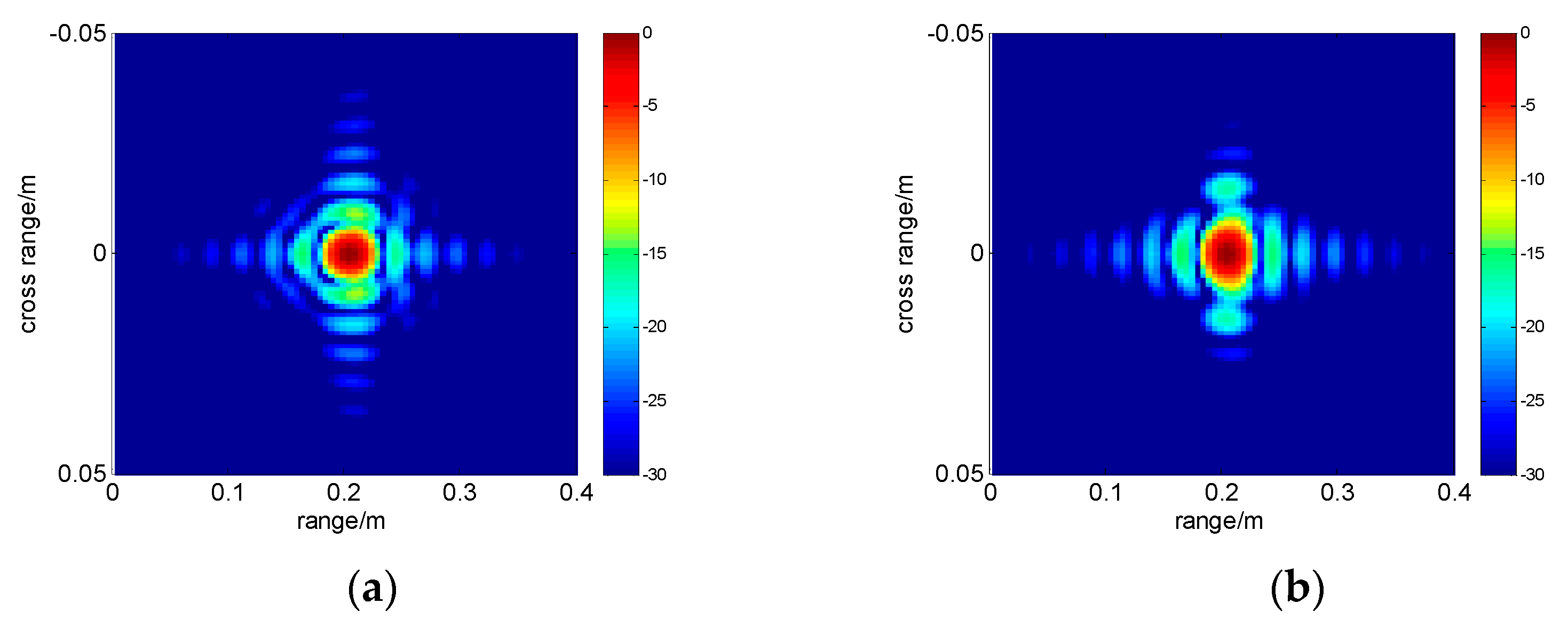
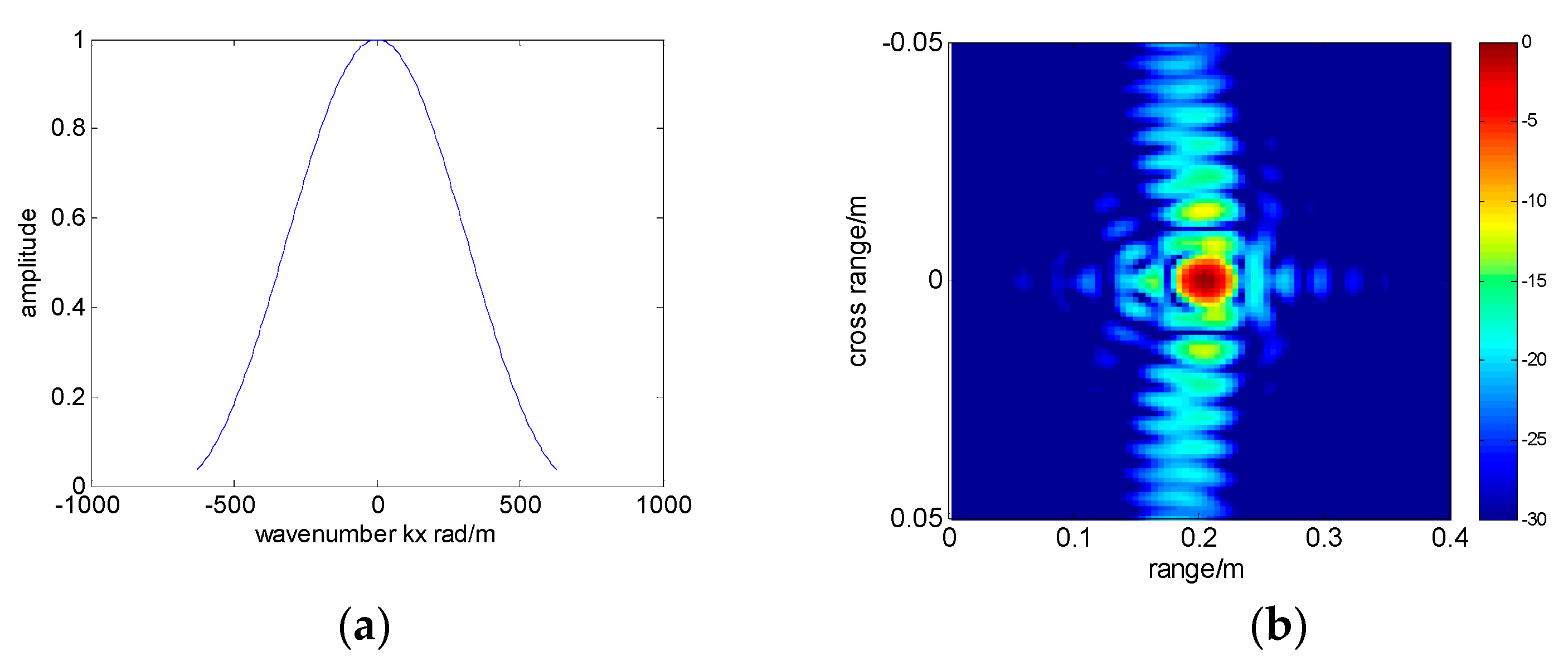
5.1. Simulation Results

Suppose that the configuration of the switch array is K = 5, M = 4, and N = 4. The operating frequency of the system is 27–33 GHz and the isolation of the switch is 10 dB. Then, the switch array can match with a 1 × 80 Tx’s antenna array and a 1 × 80 Rx’s antenna array. The point spread function of the array is simulated. The imaging results are shown in Figure 5 and Figure 6. Figure 5a,b are the PSF when the signal leakages between different channels don’t exist and exist, respectively. Figure 6 shows the comparison of the cross range PSF and the comparison of the range PSF in the two different cases, respectively. It is obvious that the signal leakages between different channels make the PSF broaden in cross range direction but it has little effect on the PSF in range direction. According to Expression (10), the PSF P_original(x,y) influenced by leaked signals is a combination of the P(x,y) shifted (i − n)λ/2 in the x direction but not shift in the y direction. The result of the superposition of several pulses with misaligned centers will be wider than the pulse before superposition, thus, the system cross resolution along the x axis is deteriorated and the range resolution along y axis is not affected. We can see that in Figure 6, the cross resolution of signal leakage is worse, and the range resolution does not change compared to the results without signal leakage. It is consistent with the analysis above.

To eliminate the influence of the signal leakage, a calibration was made according to Expression (11). The array calibration factor is shown in Figure 7a and the calibration results are shown in Figure 7b and Figure 8. The imaging result after calibration is basically the same as the result without the signal leakages. It indicates that the calibration method can eliminate the effects of leakage signals.

On the other hand, it can be found that the calibration factor is similar to a window function. Thus, the calibration process can be seen as an inverse process of windowing in the frequency domain. We can use the window function to replace the array calibration factor. We call this method the window function calibration method (WFCM). A Kaiser window with beta of 2.5 created by MATLAB shown in Figure 9a is used and the calibration result is shown in Figure 9b and Figure 10.

It can be seen that both methods can eliminate the broadening of the main lobe in the cross range. However, the side lobes raise evidently when using the WFCM method at the cross direction compared to the ACFM method described in Expression (11). It indicates that the array calibration factor created by Expression (11) can improve the image quality compared to the general window function. Impulse response width (IRW) and peak side lobe ratio (PSLR) [33] can be used to evaluate the calibration performance. The comparison of two calibration method performance is shown in

Table 1. The comparison of two calibration method performance.

Calibration Method	IRW	PSLR (dB)
Array Calibration Factor Method (ACFM)	1.008	−13.96
Window Function Calibration Method (WFCM)	1.004	−11

. IRW is normalized with its theoretical resolution, so its unit is 1. The measurement results of PSLR are also marked in Figure 10.

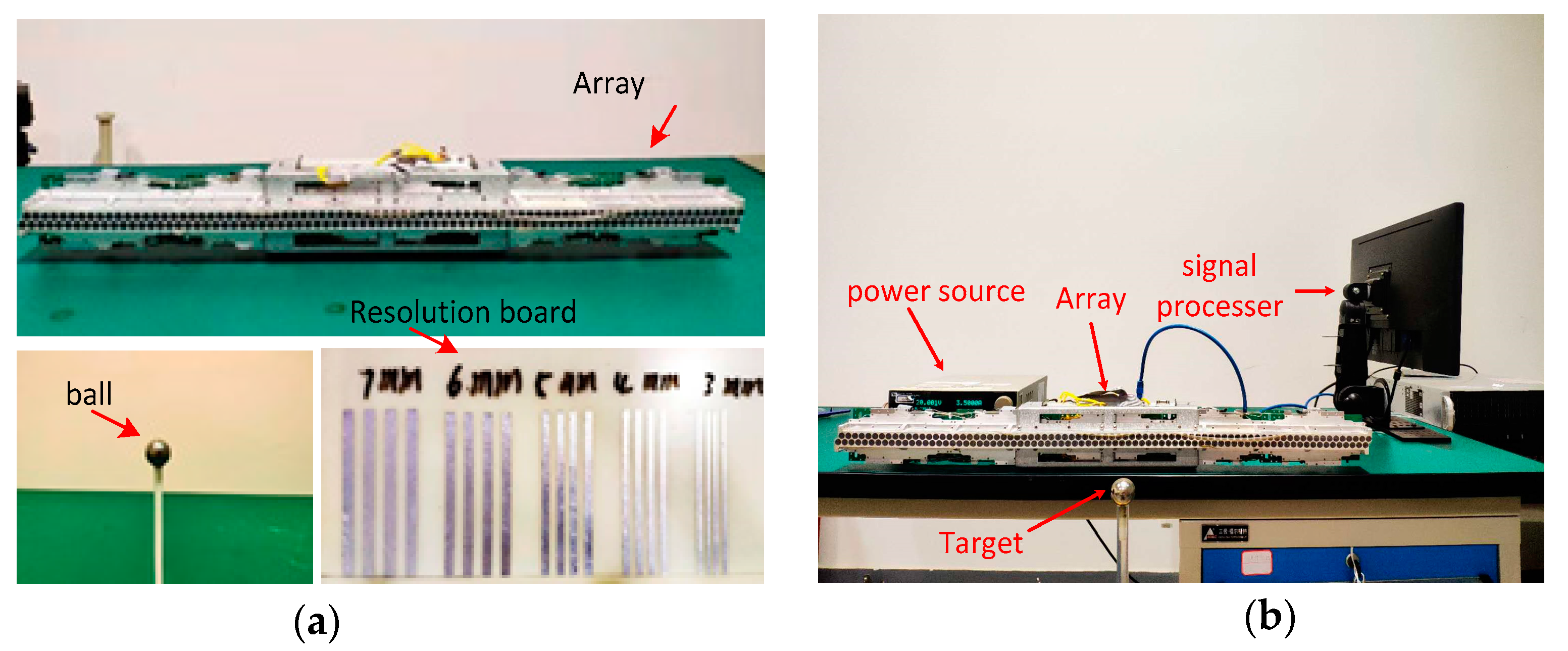
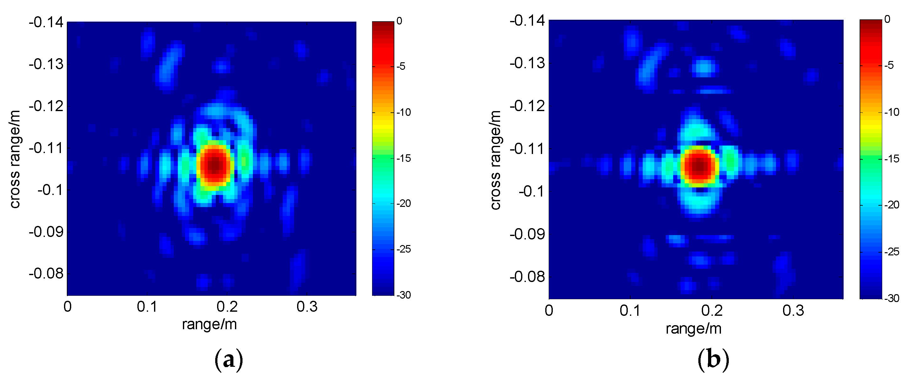
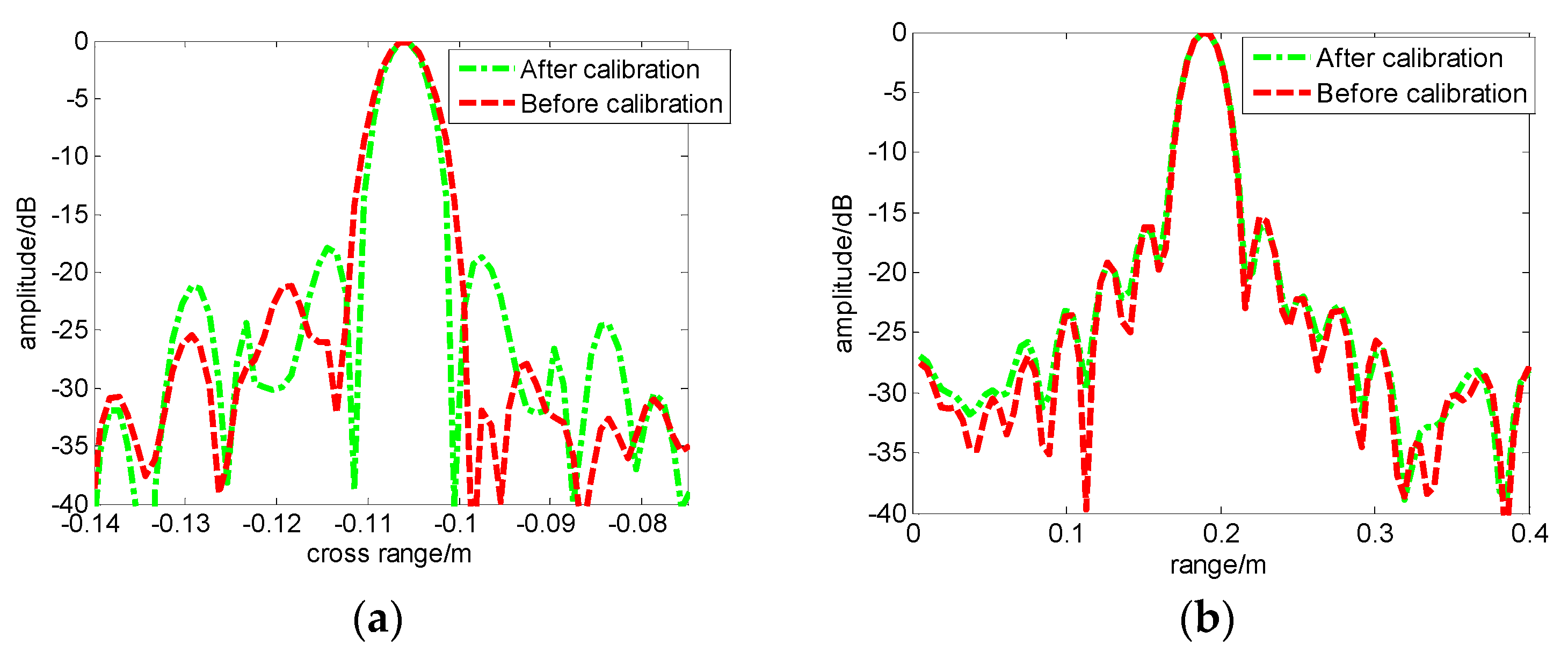
5.2. Experiment Results

An experiment was conducted to verify the effectiveness of the method mentioned above. The real array, targets, and photo of measurements in the experiments are shown in Figure 11. The configuration of the switch array is K = 5, M = 4, and N = 4. The operating frequency of the system is 27–33 GHz. The isolation of the array between different channels is about 25 dB. A two-dimension (2D) imaging was carried out with a ball shown in Figure 11, which can be seen as a point target. The results are shown in Figure 12. Figure 12a is the 2D imaging result without calibration. Figure 12b is the imaging result after calibration. Figure 13a,b are the PSF comparisons between the results before and after calibration. Obviously, it can be seen that the calibration process has an improvement on the cross-range resolution and has no impact on the range resolution. One point to note is that the calibration process improves the cross resolution and also raises the sidelobe levels. However, a set of calibration factors which is designed according to the structure of the array can bring as little side-lobe increases as possible compared to other window functions.

A simple resolution test board shown in Figure 11 was tested with three-dimension (3D) imaging. The maximum projection results are shown in Figure 14. Figure 14a shows the result without calibration. Figure 14b shows the result calibrated with the method mentioned above. We can see that the gap between the aluminum bars in Figure 14b is clearer than the gap in Figure 14a. This shows that the calibration method can eliminate most of the impacts of the signal leakage and improve the cross resolution of the system.

In this section, a simulation and some experiments are carried out to validate the effectiveness of the proposed method. The simulation and the experiment results indicate that this calibration method can mostly cancel the influence of the signal leakages.

6. Conclusions

This paper discussed the influence of the signal leakages between different channels in the application of array imaging. Signal leakage between different channels can deteriorate the system cross resolution but has no impact on the range resolution. When the channel isolation is not good enough, it will lead to the appearance of grating lobes, which we tried to eliminate in this paper. A calibration method was presented to eliminate the influences of signal leakages and was validated with the simulation and some experiments. The calibration factor proposed in this paper can better improve the image quality compared to the used window function. However, we have not yet obtained an optimal window function selection method which may obtain better calibration results. Some optimization methods can be tried in related directions. It will be carried out in future work. The effect of noise on the calibration process proposed in the paper also can be a research direction in the next work. The same analysis method and calibration method can be extended to complex array imaging application analyses.

References

1. Sheen, D.M.; Clark, R.T.; Tedeschi, J.R.; McCall, J.; Hartman, T.S.; Jones, A.M. Efficient image reconstruction method for a millimeter-wave shoe scanner. In Proceedings of the Passive and Active Millimeter-Wave Imaging XXIII, Vancouver, BC, Canada, 23 April 2020. [Google Scholar]
2. Jones, M.; Sheen, D.; Tedeschi, J. Wideband archimedean spiral antenna for millimeter-wave imaging array. In Proceedings of the 2017 IEEE International Symposium on Antennas and Propagation & USNC/URSI National Radio Science Meeting, San Diego, CA, USA, 9–15 July 2017; pp. 845–846. [Google Scholar]
3. Sheen, D.; Jones, M.; Hall, T.E. Simulation of active cylindrical and planar millimeter-wave imaging systems. In Proceedings of the Passive and Active Millimeter-Wave Imaging XXI, Orlando, FL, USA, 18–20 April 2018. [Google Scholar]
4. Meng, Y.; Lin, C.; Zang, J.; Qing, A. MMW Holographic Imaging for Security Check. In Proceedings of the 2019 IEEE Asia-Pacific Microwave Conference (APMC), Singapore, 10–13 December 2019; pp. 569–571. [Google Scholar]
5. Ma, Q.; Chung, H.; Rebeiz, G.M. A 4-Channel 10–40 GHz Wideband Receiver with Integrated Frequency Quadrupler for High Resolution Millimeter-Wave Imaging Systems. In Proceedings of the 2018 IEEE/MTT-S International Microwave Symposium—IMS, Philadelphia, PA, USA, 10–15 June 2018; pp. 883–886. [Google Scholar]
6. Cheng, B.; Cui, Z.; Lu, B.; Qin, Y.; Liu, Q.; Chen, P.; He, Y.; Jiang, J.; He, X.; Deng, X.; et al. 340-GHz 3-D Imaging Radar With 4Tx-16Rx MIMO Array. IEEE Trans. Terahertz Sci. Technol. 2018, 8, 509–519. [Google Scholar] [CrossRef]
7. Li, S.; Zhao, G.-Q.; Sun, H.; Amin, M.G. Compressive Sensing Imaging of 3-D Object by a Holographic Algorithm. IEEE Trans. Antennas Propag. 2018, 66, 7295–7304. [Google Scholar] [CrossRef]
8. Gao, J.; Qin, Y.; Beng, B.; Wang, H.; Li, X. A novel method for 3D milliter-wave holographic reconstruction based on frequency interferometry techniques. IEEE Trans. Microw. Theory Technol. 2018, 66, 1579–1596. [Google Scholar] [CrossRef]
9. Gao, J.; Qin, Y.; Deng, B.; Wang, H.; Li, X. Novel Efficient 3D Short-Range Imaging Algorithms for a Scanning 1D-MIMO Array. IEEE Trans. Image Process. 2018, 27, 3631–3643. [Google Scholar] [CrossRef] [PubMed]
10. Gao, J.; Deng, B.; Qin, Y.; Li, X.; Wang, H. Point Cloud and 3-D Surface Reconstruction Using Cylindrical Millimeter-Wave Holography. IEEE Trans. Instrum. Meas. 2019, 68, 4765–4778. [Google Scholar] [CrossRef]
11. Mirbeik-Sabzevari, A.; Oppelaar, E.; Ashinoff, R.; Tavassolian, N. High-Contrast, Low-Cost, 3-D Visualization of Skin Cancer Using Ultra-High-Resolution Millimeter-Wave Imaging. IEEE Trans. Med. Imaging 2019, 38, 2188–2197. [Google Scholar] [CrossRef] [PubMed]
12. Mirbeik-Sabzevari, A.; Li, S.; Garay, E.; Nguyen, H.T.; Wang, H.; Tavassolian, N. Synthetic Ultra-High-Resolution Millimeter-Wave Imaging for Skin Cancer Detection. IEEE Trans. Biomed. Eng. 2019, 66, 61–71. [Google Scholar] [CrossRef] [PubMed]
13. Mirbeik-Sabzevari, A.; Tavassoian, N.; Ashinoff, R. Ultra-High-Resolution Millimeter-Wave Imaging: A New Promising Skin Cancer Imaging Modality. In Proceedings of the 2018 IEEE Biomedical Circuits and Systems Conference (BioCAS), Cleveland, OH, USA, 17–19 October 2018; pp. 1–4. [Google Scholar]
14. Wang, P.; Millar, D.; Parsons, K.; Orlik, P.V. Nonlinearity correction for range estimation in FMCW millimeter-wave automotive radar. In Proceedings of the 2018 IEEE MTT-S International Wireless Symposium (IWS), Chengdu, China, 6–10 May 2018; pp. 1–3. [Google Scholar]
15. Wang, P.; Millar, D.; Parsons, K.; Ma, R.; Orlik, P.V. Range Accuracy Analysis for FMCW Systems with Source Nonlinearity. In Proceedings of the 2019 IEEE MTT-S International Conference on Microwaves for Intelligent Mobility (ICMIM), Detroit, MI, USA, 15–16 April 2019; pp. 1–5. [Google Scholar]
16. Li, Y.; Hu, W.; Zhang, X.; Zhao, Y.; Ni, J.; Ligthart, L.P. A Non-Linear Correction Method for Terahertz LFMCW Radar. IEEE Access 2020, 8, 102784–102794. [Google Scholar] [CrossRef]
17. Schiessl, A.; Genghammer, A.; Ahmed, S.S.; Schmidt, L.P. Phase error sensitivity in multistatic microwave imaging systems. In Proceedings of the 43rd European Microwave Coference, Nuremberg, Germany, 7–10 October 2013; pp. 1631–1634. [Google Scholar]
18. Pinel-Puyssegur, B.; Lasserre, C.; Benoit, A.; Jolivet, R.; Doin, M.; Champenois, J. A Simple Phase Unwrapping Errors Correction Algorithm Based on Phase Closure Analysis. In Proceedings of the IGARSS 2018—2018 IEEE International Geoscience and Remote Sensing Symposium, Valencia, Spain, 23–27 July 2018; pp. 2212–2215. [Google Scholar]
19. Deng, H.; Farquharson, G.; Sahr, J.; Goncharenko, Y.; Mower, J. Phase Calibration of an Along-Track Interferometric FMCW SAR. IEEE Trans. Geosci. Remote Sens. 2018, 56, 4876–4886. [Google Scholar] [CrossRef]
20. Korner, G.; Oppelt, D.; Adametz, J.; Vossiek, M. Novel Passive Calibration Method for Fully Polarimetric Near Field MIMO Imaging Radars. In Proceedings of the 2019 12th German Microwave Conference (GeMiC), Stuttgart, Germany, 25–27 March 2019. [Google Scholar]
21. Zhao, Q.; Zhang, Y.; Wang, W.; Wang, P.; Wang, R.; Deng, Y.; Zhang, H.; Ye, K.; Zhou, Y. Channel Imbalance Compensation with IF Signal for China’s IDBSAR. In Proceedings of the IGARSS 2019—2019 IEEE International Geoscience and Remote Sensing Symposium, Yokohama, Japan, 28 July–2 August 2019; pp. 1112–1115. [Google Scholar]
22. Shin, D.H.; Jung, D.H.; Kim, D.C.; Ham, J.W.; Park, S.O. A distributed FMCW radar system based on Fiber-Optic links for small drone decetion. IEEE Trans. Instrum. Meas. 2017, 66, 340–347. [Google Scholar] [CrossRef]
23. Lee, S.J.; Jung, J.H.; Yu, J.-W. TX Leakage Canceller for Small Drone Detection Radar in 2-GHz Band. IEEE Microw. Wirel. Compon. Lett. 2020, 30, 213–215. [Google Scholar] [CrossRef]
24. Melzer, A.; Onic, A.; Huemer, M. Self-Adaptive Short-Range Leakage Canceler for Automotive FMCW Radar Transceivers. In Proceedings of the 2018 15th European Radar Conference (EuRAD), Madrid, Spain, 26–28 September 2018; pp. 26–29. [Google Scholar]
25. Bauduin, M.; Bourdoux, A. Mixed-Signal Transmitter Leakage Cancellation for PMCW MIMO Radar. In Proceedings of the 2018 15th European Radar Conference (EuRAD), Madrid, Spain, 26–28 September 2018; pp. 293–297. [Google Scholar]
26. Arnold, B.T.; Jensen, M.A. The Effect of Antenna Mutual Coupling on MIMO Radar System Performance. IEEE Trans. Antennas Propag. 2019, 67, 1410–1416. [Google Scholar] [CrossRef]
27. Colon-Diaz, N.; McCormick, P.M.; Janning, D.; Bliss, D.W. Compensation of Mutual Coupling Effects for Co-located MIMO Radar Applications via Waveform Design. In Proceedings of the 2019 International Radar Conference (RADAR), Toulon, France, 23–27 September 2019; pp. 1–6. [Google Scholar]
28. Chen, X.; Zhang, S.; Li, Q. A Review of Mutual Coupling in MIMO Systems. IEEE Access 2018, 6, 24706–24719. [Google Scholar] [CrossRef]
29. Sheen, D.; McMakin, D.; Hall, T. Three-dimensional millimeter-wave imaging for concealed weapon detection. IEEE Trans. Microw. Theory Tech. 2001, 49, 1581–1592. [Google Scholar] [CrossRef]
30. Kell, R. On the derivation of bistatic RCS from monostatic measurements. Proc. IEEE 1965, 53, 983–988. [Google Scholar] [CrossRef]
31. Stolt, R.H. Migration by Fourier Transform. Geophysics 1978, 43, 23–48. [Google Scholar] [CrossRef]
32. Jiacheng, S.; Chen, M. Research on Imaging Algorithm of Millimeter Wave Radar Based on Stolt Interpolation. In Proceedings of the 2019 IEEE MTT-S International Microwave Biomedical Conference (IMBioC), Nanjing, China, 6–8 May 2019; pp. 1–4. [Google Scholar]
33. Cumming, I.G.; Wong, F.H. Digital Processing of Synthetic Aperture Radar Data Algorithms and Implementation; Artech House: Boston, MA, USA, 2005; pp. 39–41. [Google Scholar]
Figure 1. Array configuration of the transmitting and receiving elements.
Electronics 09 01628 g001
Figure 2. RF switch network.
Electronics 09 01628 g002
Figure 3. Signal path form Tx to Rx.
Electronics 09 01628 g003
Figure 4. The Fourier transform of ui(n).
Electronics 09 01628 g004
Figure 5. Simulated PSF in two different cases, (a) is the PSF when the signal leakages do not exist and (b) is the PSF when leakages exist.
Electronics 09 01628 g005
Figure 6. The comparison of PSF in two different dimensions, (a) is the cross range PSF and (b) is the range PSF.
Electronics 09 01628 g006
Figure 7. The array calibration factor and the imaging result after calibration, (a) is the array calibration factor and (b) is the imaging result after calibration.
Electronics 09 01628 g007
Figure 8. The PSF comparison of three different cases, (a) is the cross range PSF and (b) is the range PSF.
Electronics 09 01628 g008
Figure 9. The Kaiser window with beta of 2.5 and its calibration result, (a) is Kaiser window and (b) is the calibration result.
Electronics 09 01628 g009
Figure 10. The PSF comparison of different cases in cross range and range, (a) is the cross range PSF and (b) is the range PSF.
Electronics 09 01628 g010
Figure 11. The array, targets and photo of measurements in experiments, (a) is array and targets; (b) is the experiment scene.
Electronics 09 01628 g011
Figure 12. 2D imaging result of the ball in experiments, (a) is the imaging result before calibration and (b) is the imaging result after calibration.
Electronics 09 01628 g012
Figure 13. The PSF comparisons of the ball in experiments before and after calibration, (a) is the cross range PSF and (b) is the range PSF.
Electronics 09 01628 g013
Figure 14. Imaging results of the resolution board in experiments before and after calibration, (a) is the imaging result before calibration and (b) is the imaging result after calibration.
Electronics 09 01628 g014