1. Introduction
Underwater Wireless Sensor Networks (UWSN) is an important research field devoted to providing scalable and flexible platforms for a wide range of underwater applications. Some of these applications are related to oceanic monitoring, underwater positioning, and Autonomous Underwater Vehicles (AUV) [
1]. Currently, there are three main technologies capable of operating in underwater environments: Underwater Acoustic Communication (UAC), Underwater Wireless Optical Communication (UWOC), and Underwater Radio Frequency Communication (URFC).
Traditionally, underwater wireless communication has been carried out using pressure waves. UAC is a very well-studied topic in which information is transmitted using acoustic signals which propagate long distances (kilometers) through seawater. The low losses that the medium presents produce severe multi-path responses (several reflections on both seabed and surface), reducing the coherence bandwidth and hence the maximum achievable data rate [
2]. Furthermore, the underwater acoustic channel suffers from saturation, a significant human-generated noise background level, and the possibility of harming cetaceans if the used carrier frequencies are below 200–300 KHz [
3].
UWOC provides very high data rates at short or medium distances (up to 100 m approximately) [
4,
5], and the link quality greatly depends on the alignment between endpoints. Nonetheless, these misalignment restrictions are more relaxed than expected thanks to scattering [
6]. The exponential losses due to light-matter interaction limit the use of this technology to a few meters in UWSN applications (and depends on the working wavelength). Moreover, the optical emission is generally confined to a reduced solid angle, usually limiting the potential network-associated graphs to directed ones [
7]. Nevertheless, some authors have tried to overpass this limitation by emulating isotropic radiation using angular diversity techniques at the nodes [
8]. This solution reduces cost-efficiency, increases the node’s intelligence complexity, and finally shortens the node’s lifespan due to the excess energy consumption.
The use of ElectroMagnetic (EM) signals to establish underwater communication links is a promising field of study. There are two main techniques within this broad technology. On the one hand, terrestrial Radio Frequency (RF) systems can be adapted to underwater environments. However, in this case, communication relies mainly on the electric field, suffering from very high attenuation due to the loss tangent of seawater and Doppler spread [
9]. This dramatically limits both link range and data rate. On the other hand, Magnetic Induction (MI) provides higher robustness, allows higher bandwidth (up to Mbps), and it primarily depends on the seabed’s conductivity [
10]. This work focuses on the latter, and the associated propagation model will be more in-depth analyzed in
Section 4.
UWSN communication protocols determine several capital aspects of the network performance, such as throughput, packet delay, robustness, and the network’s lifespan. JANUS, which is currently the most adopted communications standard in UAC, was motivated by the necessity of inter-operability between manufacturers [
11]. Nonetheless, the specifications of JANUS may not be applicable to other technologies, since they were designed taking into account the underwater acoustic channel behaviour. On the other hand, STANAG 5066 is a military communication standard (STANdard AGreement 5066) focused on optimising low-throughput and low-reliability communications. It is one of the most common and widely used High Frequency (HF) communication protocols for military applications. These characteristics turn this protocol into a serious candidate for EM-URFC UWSN applications.
The simulation of UWSNs has been traditionally carried out using network-level platforms with simplified Medium Access Control (MAC) and Physical (PHY) layers. These simulators provide a high-level interface in which the behavior of the lower layers must be defined ad hoc since the protocols do no work in real-time but in an event-driven manner. Therefore, this approach limits the capacity of testing real-world MAC and PHY implementations. On the other hand, software-in-loop is a paradigm in which a piece of software can be tested within a controlled environment respecting its timing structure.
In this work, a
software-in-loop system capable of simulating the real-time operation of an EM-UWSN based on a STANAG 5066 communications stack is presented. This STANAG 5066 stack is embedded into the development of an actual underwater sensor node, framed within the Spanish Research Administration project HERAKLES. This project has two main objectives. On the one hand, it aims to study the propagation of EM signals in underwater environments, both theoretically and experimentally. On the other hand, it proposes the development of a Multiple Input Node Interface for Offshore Networking (MINION) as the building block of an UWSN.
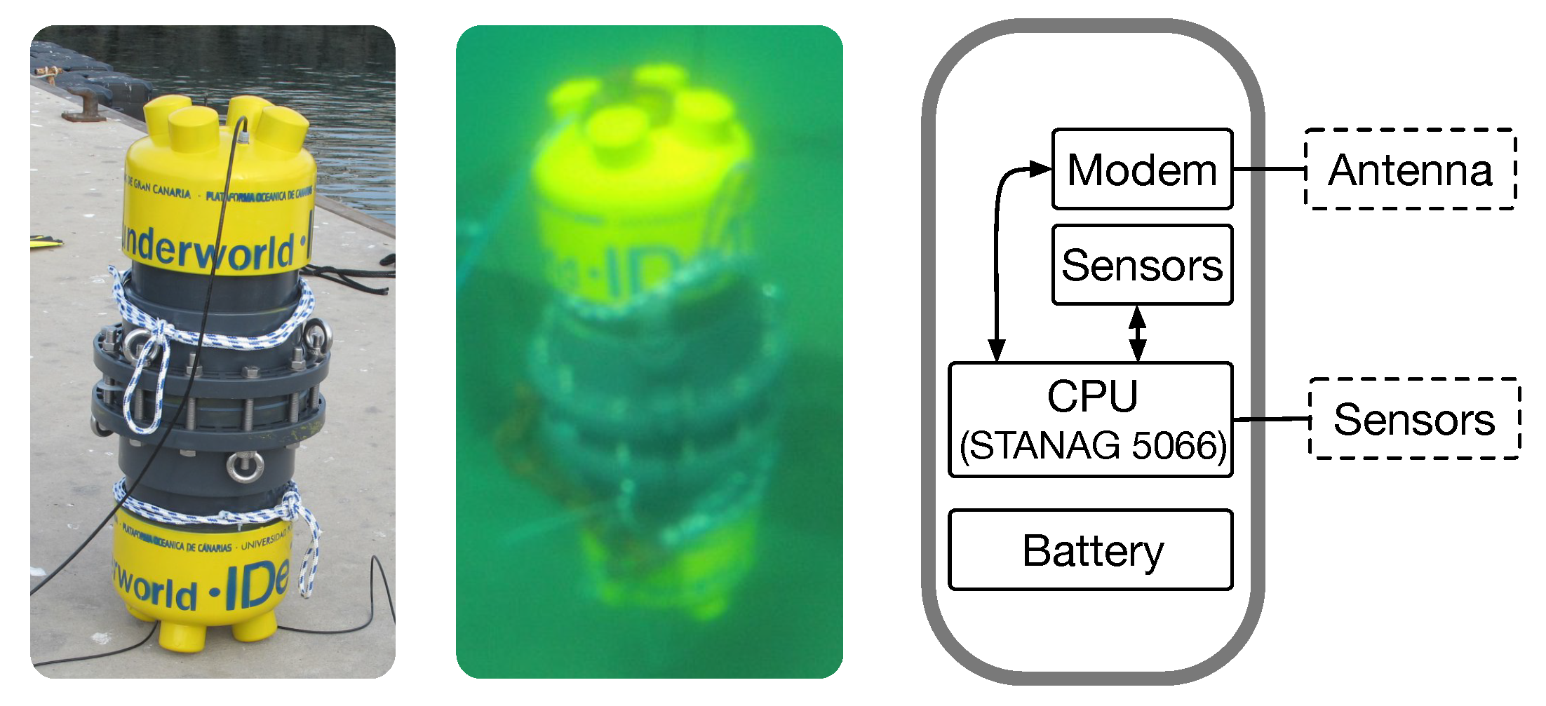
Figure 1 depicts the actual design of the underwater node. This paper focuses on the development of a
software-in-loop platform capable of simulating the behavior of an underwater network of MINIONs, which uses a real-implementation of the STANAG 5066 stack.
With the final objective of embedding the developed STANAG 5066 stack into a real UWSN deployment, a simulator capable of handling the communication of 20 virtual nodes simultaneously was implemented. This simulator allows the execution of the software that will be actually running inside each MINION, without any modification. Unlike other simulation schemes such as discrete event processing, in which framework-specific implementations of STANAG 5066 would have been needed, the proposed scheme is characterized by the complete reuse of the developed software.
This paper is structured as follows—
Section 2 provides a comprehensive analysis of the state-of-the-art solutions regarding UWSN simulation.
Section 3 introduces the NATO STANAG 5066 protocol and describes its particularities. The electromagnetic underwater propagation model considered in this paper is presented in
Section 4. The
software-in-loop system developed in this work is in-depth presented in
Section 5. The methodology used to demonstrate the feasibility of the proposed
software-in-loop approach, and the obtained experimental results are presented in
Section 6 and
Section 7 respectively. Finally, the results are in-depth discussed in
Section 8, and some conclusions are extracted in
Section 9.
2. Related Work
Simulation of UWSN is an important research topic due to its impact on the design and optimization of these networks, which normally have prohibitive node-replacement costs [
12]. Wireless networks are usually simulated with different detail levels, using event-driven approaches that reduce the resulting simulation time. Frameworks such as Castalia, NS-3, OMNeT++, or OPNET are employed to simulate MAC protocols and network algorithms, using specific event-driven implementations [
13]. Therefore, these frameworks do not offer the possibility of testing a given real-world implementation of a communications stack under a realistic scenario. Lalomia et al. carried out a soft real-time simulation of a WSN, merging both virtual and actual sensor nodes [
14]. In their scheme, the authors did not handle communication in a concurrent or parallel manner, incurring sometimes into timing errors. The simulator proposed in this paper is inherently concurrent and easily parallelizable, minimizing this type of error. Saginbekov and Shakenov analyzed in Reference [
15] some hybrid network simulators, capable of handling interaction between physical and virtual nodes. The authors analyzed these frameworks in terms of scalability, synchronization, Graphical User Interface (GUI), and source emulation capability. This last parameter is related to the capacity of executing exactly the same code in both virtual and physical nodes. Although H-TOSSIM [
16] and MULE [
17] are capable of synchronized execution and source code emulation, they need from a specific communication protocol that must be embedded into the real-deployed node (on the contrary, a pure
software-in-loop approach ensures that the protocol that is running on the simulated node will be the same on a real scenario).
Saginbekov and Shakenov’s analysis included not only traditional Discrete Event Simulators (DES), but also frameworks capable of hybrid simulation (virtual and real nodes). Nonetheless, this kind of simulators does not offer the possibility of testing real software before carrying out the physical implementation of the nodes. On the other hand, Naumann et al. studied several schemes capable of protocol emulation in Reference [
18]. The authors distinguished between platforms that allowed partial code reuse and full code reuse. The full reuse objective can be reached using a Software Compatibility Layer (SCL) or by the use of alternative compilation (using shared libraries). SCL provides a higher level of abstraction for network simulation, but the source code must be designed taking this into account
a priori. The Click modular router [
19] provides a modular Application Programming Interface (API) that can be used to design new protocols. However, the applicability of this API for existing protocol adaptation is practically unfeasible, due to the tight integration requirements of Click. Erazo et al. used a Click-based implementation of router modules to carry out a realistic Ethernet network simulation [
20]. Nevertheless, the authors did not compare their results against a real-world deployment of the network under study, but only with respect to the output of a DES. Chitre et al. presented an implementation of a design tool for UWSN named UnetStack [
21]. The underlying concept of this scheme was very similar to Click. Their approach proposed the use of an agent-based architecture for implementing protocol stacks. Nonetheless, as occurred with Click, UnetStack constrains the design procedure, limiting its relevance.
Sharma et al. carried out a comprehensive comparison of DES for WSN simulation [
22]. Several frameworks such as OMNET++, NS-2, NS-3 and MATLAB were analyzed through literature review and experimental evaluation. The authors found that MATLAB offered the lowest simulation time for the Ad hoc On Demand Vector (AODV) protocol benchmark. This metric was remarked as capital for network design in their comparative study. Nonetheless, the considered frameworks and schemes were not evaluated in other terms, such as robustness and accuracy. Although the authors focused on the analysis of DES frameworks, they proposed a list of characteristics that a good network simulator must have. The list comprised simulation-specific metrics such as robustness, scalability, and accuracy, and others related to visualization and support. From a testing and validation viewpoint, DES is usually subject to the quality of the used simplified models. Therefore, their robustness and accuracy are normally below other approaches such as
software-in-loop and hardware-in-loop schemes.
The aforementioned schemes and frameworks were focused on providing a higher abstraction level for protocol implementation. However, they did not offer the possibility of evaluating already-existing protocol stacks. Unlike UnetStack, MULE, HTOSSIM, or Click, this work’s network simulation proposal treats the protocol stack as a black box, interacting at byte level.
Table 1 shows a comparison between the presented frameworks.
Routing algorithms are a fundamental part of WSN since they greatly define the network’s lifespan. The research community has traditionally put a significant amount of effort on this topic and the proposals are generally evaluated using network simulation frameworks [
23,
24,
25]. This approach is interesting when both MAC and PHY layers are well-known and are properly modeled [
26]. UWSN (and WSN in general) research has relied on this assumption. However, in most cases new MAC protocols are proposed, and performance estimation of actually-deployed nodes using event-based simulation is unfeasible. Climent et al. developed an UWSN simulation environment based on NS-3 for UAC [
27] in an attempt to model real hardware. The framework included not only PHY and MAC modeling, but also weather conditions since they severely affect the communications performance of ultrasound-based underwater links. Furthermore, energy-harvesting capabilities on the deployed nodes were also simulated. The authors included a detailed energy consumption framework considering different events such as wake-up, reception, idle state, and transmission, allowing a fine analysis of the network. Nonetheless, the authors only tested a star-like topology and source code emulation was not supported.
STANAG 5066 has been widely used in military maritime communications. In theory, this stack is capable of supporting common network-level protocols such as IP. Gillespie et al. analyzed the feasibility of using STANAG 5066 to support e-mail applications [
28]. The authors compared the performance of IP-over-HF and proxy agents such as HMTP or CFTP. The experimental results suggested that proxy agents provide higher throughput due to their robustness against packet delay, which is an important issue in HF communications due to the reduced bandwidths and the harsh channel. In their following work, Trinder and Gillespie simulated how the ARQ parameters of STANAG 5066 may affect performance [
29]. The authors observed that the optimum frame size depends on the channel’s average Signal-to-Noise Ratio (SNR). Taking into account the variability of the HF channel, the authors concluded that an adaptive algorithm should improve the overall performance.
Nieto studied the impact of using the high data rate HF waveforms of STANAG 4539 on STANAG 5066’s performance [
30]. This work was motivated by the need to improve the HF communications’ throughput. Nieto carried out several experiments in which interleaver, message, and packet sizes were varied, providing some recommendations as key outcomes. Although STANAG 4539 defines six interleaver lengths, the author recommended to use only Long (4.305 s for fading channels) or Short (1.07625 s in AWGN channels) configurations, as well as keeping the packet size for long messages between 6000 and 8000 bits. As it usually occurs in HF, the packet delays are high, and these recommendations help in alleviating this issue.
In a similar work, Raos et al. studied the optimization of the ARQ parameters of STANAG 5066 when used in an HFDVL (HF Data+Voice Link), which relies on Orthogonal Frequency Division Multiplexing (OFDM) with 16-QAM symbols and 73 sub-carriers [
31]. The main analyzed parameter was the presence of spatial diversity on the reception side, although ARQ parameters were also evaluated. Unlike Trinder and Gillespie, the authors carried out an experimental evaluation, resulting in a big marginal performance improvement from one antenna to two antennas. In Reference [
32], Koski et al. carried out TCP over STANAG 5066 simulations using OMNeT++. The authors focused on properly simulating the physical behavior, including a specific layer dedicated to MIL-STD-188-110C narrowband HF waveforms. The results were focused on analyzing the impact of different TCP settings on the system performance under several channel conditions, as Raos et al. in Reference [
31]. After detecting the susceptibility of TCP to the huge ionospheric SNR variations, which generate retransmissions and hence big delays, the authors proposed a Performance Enhanced Proxy to mitigate this effect with successful results.
3. STANAG 5066
STANAG 5066 is a military communication standard (STANdard AGreement 5066), developed focusing on the optimization of low-throughput communications and low-reliability channels. It is one of the most common and widely used HF communications protocols for military applications.
The HF communication channel is characterized by its harshness. It presents a high base noise, as well as selective frequency and Doppler effects. This channel has been traditionally limited to a channel bandwidth, which severely limits the maximum theoretical throughput of any HF link.
STANAG 5066 standard defines a communication protocol focused on providing both efficiency and reliability to applications communicating using an HF channel. This standard defines its own reliability-enhancement mechanisms, codification, and data encapsulation. As it was presented in
Section 1, project HERAKLES decided to use STANAG 5066 due to the reduced reliability of EM-based UWSN.
STANAG 5066 definition divides the protocol into three well-differentiated layers, Subnetwork Interface Sublayer (SIS), Channel Access Sublayer (CAS) and Data Transfer Sublayer (DTS). SIS is the layer that handles the communication between applications and STANAG 5066 stack. Therefore, it is mandatory that applications using STANAG 5066 stack implement the SIS communication protocol defined by the standard. The SIS layer defines a list of encoding structures in which payload data, such as destination address and transmission mode, are encapsulated. These data inform the STANAG 5066 stack about how the information should be managed. In the same way, the STANAG 5066 stack informs the application layer about using the same SIS protocol, indicating the origin address, transmission mode, and other metadata [
33].
STANAG 5066 protocol has two main features that should be remarked. The first feature is its extended data addressability that uses unique address assignation for each node, node group, or broadcasting. The allowed address range goes from 1 to 268,435,456 (00:00:00:01 to 0F:FF:FF:FF), whilst address zero is identified as the broadcast address. This means that up to (more than 268 million) nodes with a unique address could be deployed. This feature guarantees with a high significance level that address collisions are essentially avoided. This characteristic is of high relevance in the underwater scenario in which STANAG 5066 stack is being proposed in project HERAKLES.
The second feature is that STANAG 5066 standard defines two differentiated transmission modes: ARQ and NONARQ. Both ARQ and NONARQ modes use Cyclic Redundant Code (CRC) to identify the integrity of the received data. Furthermore, if the data payload is larger than a configurable amount of bytes, STANAG 5066 carries out data fragmentation into chunks with their CRC codes. Data reassembly is carried out also by the STANAG 5066 stack at the receiver side. The chunk size selected in this work was 100 bytes, based on previous analysis made by Raos et al. [
31].
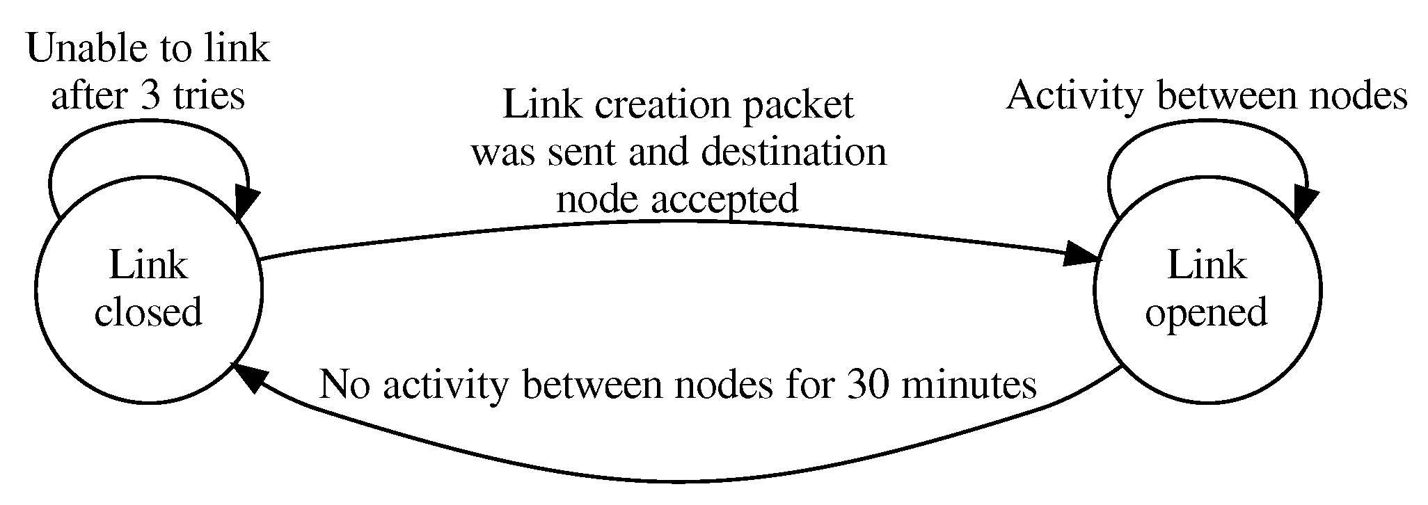
ARQ transmission mode implements Selective Repeat ARQ techniques to perform the retransmission of packets that have been received with errors (or even not received), guaranteeing that information, when received, is sent to upper layers without errors. STANAG 5066 defines a handshake procedure between endpoints before any ARQ message is transmitted. This operation is automatically managed by STANAG 5066 stack, and it establishes a link between both sender and receiver. This link is considered to be active unless 30 minutes of inactivity are reached. The behaviour of the link creation and destruction is depicted in
Figure 2.
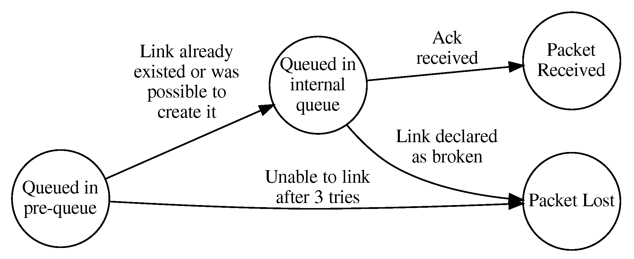
The process that an ARQ message follows is illustrated in
Figure 3. A packet will be considered as lost if the link is unable to be created (as explained above), or if its corresponding acknowledge is not received. If the link is active, the queued messages are retransmitted until the link is declared as broken. If no ACK is received, a uniformly distributed back-off period ranging from 250 ms to 4 s is waited before the next retransmission. The maximum back-off period is doubled after each try.
NONARQ transmission mode uses CRC and segmentation to detect whether the data have been received without errors. Using SIS protocol metadata, transmitter nodes can set NONARQ segments to be retransmitted from 1 to 15 times. During reception, NONARQ data can be reassembled using error-free segments in first place, segments with errors, or even not received ones (padded with binary-zero data) using SIS protocol metadata flags that inform the application about which data parts have present errors.
STANAG 5066 sets an upper boundary for both ARQ and NONARQ transmission modes, limiting the maximum transmission window to 60 s. During this time, each node is allowed to transmit all the queued messages that fit into the aforementioned window. After the transmission window, it is mandatory for STANAG 5066 nodes to stop during an implementation-dependent period before transmitting more data. In this work, the implemented STANAG 5066 protocol stack has been configured for waiting during an uniformly-distributed random time ranging from 250 ms to 4 s (as the ARQ back-off time).
The developed executable binary was developed and compiled to be run under GNU/Linux operating systems, and both to-phy (or its software driver) and to-application communications are driven through a TCP/IP socket. Thus, applications that pretend to use the implemented STANAG 5066 stack will have to implement SIS protocol over a TCP/IP socket. The STANAG 5066 stack implementation has already defined some implementation-dependant characteristics, such as segment sizes or internal timing.
The use of STANAG 5066 standard fits the scenario under consideration in this work. This protocol was designed for low-throughput and high-latency scenarios, and the channel capacity associated with EM underwater propagation, as well as the hardware of the implemented physical devices, fit the characteristics that STANAG 5066 standard has been designed for.
4. Electromagnetic Underwater Propagation Model
Electromagnetic waves in EM bands generally suffer from a high tangent loss in seawater (Equation (
1)) [
34]. These high dielectric losses are closely related to the medium’s conductivity
(which depends on temperature and salinity) and the behavior of the electrical permittivity
with frequency, which is generally described using Debye’s relaxation model (Equation (
2)).
and are the static and optical-range electric permittivity, respectively. is the relaxation time, is the dielectric constant of vacuum, and denotes angular frequency.
EM-URFC can be carried out using two main approaches. On the one hand, terrestrial RF equipment can be adapted to the underwater medium using an appropriate enclosing and adjusting the antennas. This technique relies on the electric field and is highly affected by the aforementioned effects, allowing only short range links [
35]. On the other hand, Magneto-Inductive URFC (MI-URFC) relies on the magnetic field, which suffers from a lower attenuation in seawater although its intensity is
a priori lower than the electric field. Jouhari et al. identified MI-URFC as an enabling technology for UWSN [
1].
In this work, a MI-URFC-based UWSN is proposed. The parametric model described in Equation (
3) [
36] has been used in order to determine the received power associated to each transmission event in the
software-in-loop simulator.
where
is the estimated loss at distance
d (in dB),
is a reference distance,
is a coefficient related to the medium’s absorption,
is a coefficient related to the exponent of the geometrical loss, and
X is a random variable which follows a zero-mean normal distribution with empirically-determined standard deviation
. The parameters used in this study are the same as the ones used in Reference [
36], and can be observed in
Table 2.
5. Proposed Software-in-Loop System
One of the greatest advantages of software-in-loop over hardware-in-loop is that there is no need for actually building all the nodes to simulate complex networks whilst maintaining the capacity to test critical software. Moreover, testing real embedded software instead of carrying out system-level or traditional network simulations allows a faster and more efficient debugging.
In a hardware-in-loop simulation, all the nodes have to be physically built. A hardware-in-loop simulator takes the modulated signal generated by each node as inputs and generates a real-time combined signal for each node as output. That means that the border line between implementation and simulator is located in the electrical domain, between modem and radio. The modem’s output signal, in this case, is not connected to an actual radio emitter, but to the simulation/emulation platform. On the contrary, in a software-in-loop simulation there is no need to build any node since the simulated interface is in the digital domain, and it is located between the CPU’s data interfaces and the modem. Under this scheme, the software-in-loop simulator receives and processes the bits that should be received by the system’s modem, instead of electrical signals. In this case, channel propagation and transceiver behavior are simulated, since the emphasis is put on how the software handles information.
For the software-in-loop simulation proposed in this paper, an ad hoc simulator has been developed. Usually, channel simulators are event-driven and it is not feasible to integrate external developed-and-compiled communication protocols. As STANAG 5066 is implemented and built on its own executable ELF binary, it is not possible to integrate STANAG 5066 stack (nor its events) in an event-driven simulator, as the implemented stacks have a significant amount of temporized events which highly rely on Operating System (OS) calls and are managed internally by the executable. It is obvious that any event-driven simulator must have knowledge about the temporized events in any software that runs in the complete simulation environment since it has to be able to queue them into its internal event list. This does not happen with compiled software that manages its temporized events with OS resources.
5.1. Software-in-Loop Scheme
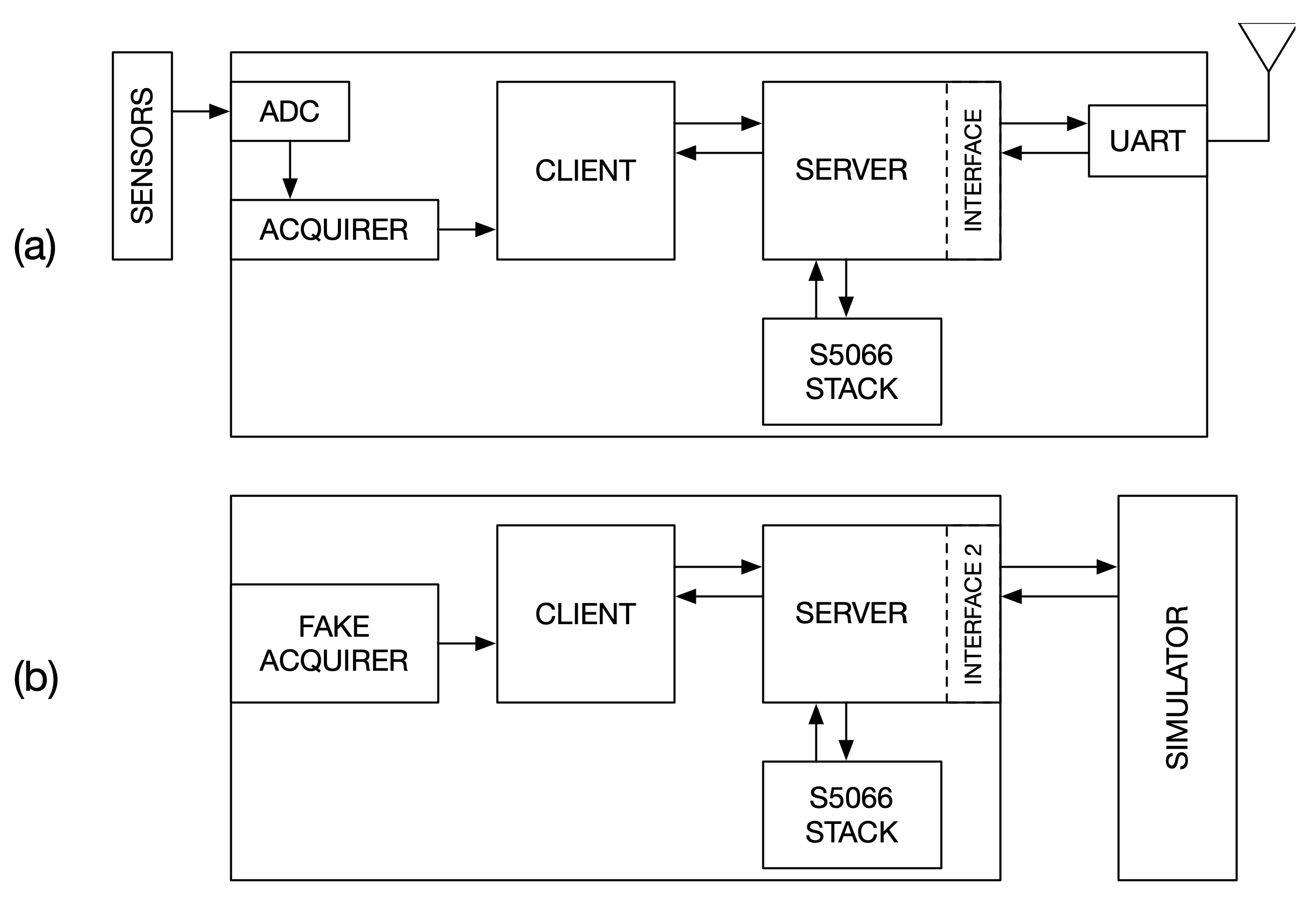
The original (not
software-in-loop) software architecture of the underwater node, shown in
Figure 4a, comprises three main executable software programs: client, server, and STANAG 5066 stack. These processes communicate between them using TCP/IP sockets. Acquirer is a Python script that reads sensor values from a UART, and also uses TCP/IP to send the fetched data to the client.
Both client and STANAG 5066 stack programs need no modification to be integrated under the proposed real-time simulation scheme. Thus, the same version of both programs is used either for deployment and for
software-in-loop simulation. Acquirer and interface are the only two software blocks in the server program that have to be adapted. A new server interface was coded in order to handle the incoming and outgoing data of the simulator, instead of handling it on a physical modem. Acquirer was changed by a
fake acquirer, because there are no available sensors in the simulated environment
Figure 4b. The characteristics of the fake acquirer are explained in
Section 6. In essence, the system’s software dependency on a real node platform (software does not need to access a real modem neither real sensors) has been removed, allowing it to run in a common PC, in a hardware-agnostic manner. Furthermore, several nodes can be simulated in a single PC.
In order to complete the software-in-loop simulation scheme, it is necessary to define how the simulator communicates with the new server interface.
A simulator has been specifically designed as part of the simulation environment developed for this work. This software block is necessary because the software inside the loop is a real-time stack (STANAG 5066), and it was not possible to integrate it with a DES. These simulation environments use next-event time progression techniques for accelerating time between different queued events. Nonetheless, the platform must be omniscient, since all the queued events are internally handled. These simulators require the specific implementation of all the software to be tested using the simulator API, which is time-consuming and does not offer the possibility of evaluating real-time software under controlled environmental conditions. These restrictions are completely incompatible with the use of STANAG 5066 stack, as this software is compiled under GNU/Linux OS, and it uses its own event queue and timing integrated with OS system calls.
The simplified simulation algorithm is depicted in
Figure 5. This algorithm shows that the simulator can be considered as a DES using fixed-increment time progression (resembling a continuos simulation scheme), but every time slice is incremented in real-time. The size of the time increment is represented by
. Internal simulator events represent transmissions made by any node. Once the transmitted message (using the server’s interface) is received by the simulator, it adds the message to the internal event queue. Then, all the queued messages are consumed in
steps. The remaining data is still queued to be consumed in the future. If there is no queued event, a wait cycle is performed. The selection of
value is a trade-off between computational efficiency and real-time event handling capacity. Small values (1 to 50 ms) of
imply that an event-handling cycle is performed very frequently. Therefore, the simulator program will take a high CPU usage. For higher values of
, the CPU usage will decrease, but transmissions that were generated within the handling cycle will be time-aligned to the next starting cycle. For instance, if
s is considered, all the transmissions started by any node during the current 1-second handling cycle will be managed in the following cycle, all of them aligned at the same time. A value of 25 ms was selected, as STANAG 5066 have a randomized medium access time with increments of 25 ms.
One of the positive aspects of this approach is that any asynchronous (from a simulator point of view) event generated by any STANAG 5066 stack (by any node), will be pseudo-immediately inserted into the event queue, and the event consumption will start in the very next data block.
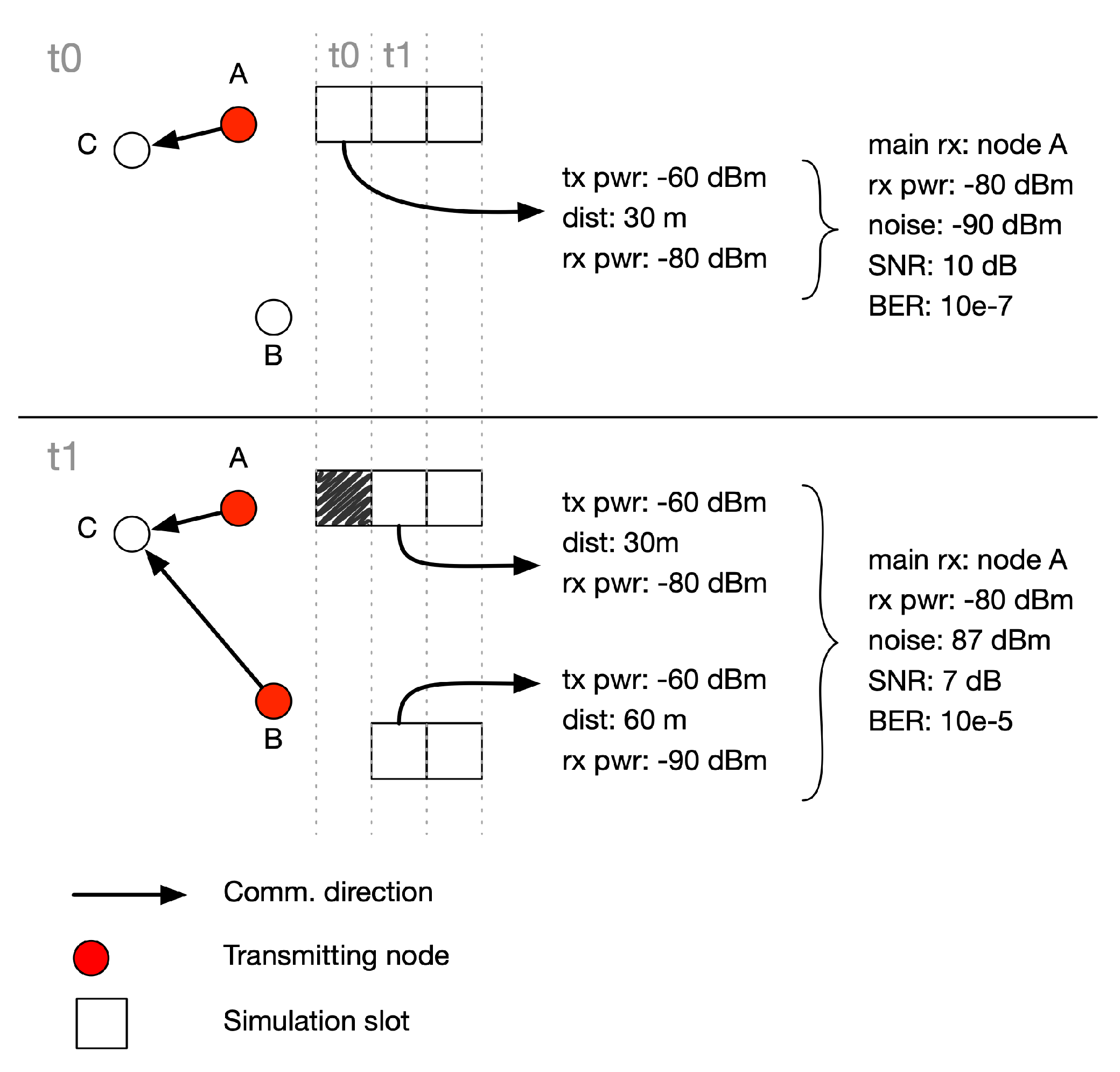
Going into detail, every internal simulator event represents a transmission made by some node with all the binary data to be transmitted on it. In a real transmission case, the server interface software will ask the UART driver to make the transmission, and the UART driver will perform the data transfer to the physical UART. This is now performed by the simulator, to whom the re-coded server interface software sends its complete data stream, and the simulator will pick 25 ms of bitstream at the configured modem speed. Additionally, this transmission event has other metadata attached to it, such as transmission power or transmission radio frequency.
5.2. Channel Simulation
Event processing is implemented from a receiver viewpoint, and the associated algorithm can be observed in Algorithm 1. For every receiver, the most powerful reception among all the queued events (transmissions) is marked as the preferential transmission and is described by
. The parametric model described in Equation (
3) [
37] is used in order to determine the received power associated to each event. All the other transmissions are considered as interference and will be summed up together under the assumption of uncorrelation in addition to the receiver’s thermal noise
, to determine the overall noise power (Equation (
4)).
I is the set comprising all the received powers except the one marked as preferential. Once the Signal-to-Interference-and-Noise ratio (SINR) is calculated, the Bit Error Rate (BER) is estimated for the current modem used by the receiver taking into account the modulation format. The physical modem used in HERAKLES’ nodes is a CML Microcircuits modem. Therefore, a non-coherent Frequency Shift Keying (FSK) demodulator must be considered (Equation (
5)). Moreover, a bit-wise xor operation with a uniformly generated bit mask is performed to the preferential transmission within the 25 ms block in order to simulate errors. The xor mask is randomly obtained taking into account statistical uniformity in the position of the reception errors. Furthermore, the number of errors to be introduced on each event follows a Binomial distribution. After carrying out this process for all the non-transmitting nodes, 25 ms of bits (using modem throughput) will be deleted from every queued event. Taking into account this consideration and the frame length
N, the Packet Error Rate (PER) can be expressed as shows Equation (
6).
| Algorithm 1 Simulator main loop | |
|
Set | |
| while True do | ▹ Main loop, so run until program ends
|
|
| |
|
for all do | ▹ Check for new transmissions
|
|
if StartedTransmission(s) then | |
|
Set | |
|
Append | |
|
end if | |
|
end for | |
|
for all do | |
|
if n) then | |
|
skip n | |
|
end if | |
|
Set | |
|
Set | |
|
Set | ▹ As described in Equation (3) |
|
Set | |
|
Set | ▹ As described in Equation (5)
|
|
Set | ▹ Randomize bitstream
|
|
call n.send()
| |
|
end for | |
|
Set | |
|
Set | |
|
sleep | ▹ Sleep only if , otherwise prints an error
|
| end while | |
| functionFindMostPowerfulReception()
| |
|
Set | |
|
Set | ▹ Power is in dBm
|
|
for all do | |
|
Set | |
|
Set | |
|
if then | |
|
Set | |
|
Set | |
|
end if | |
|
end for | |
|
return | |
| end function | |
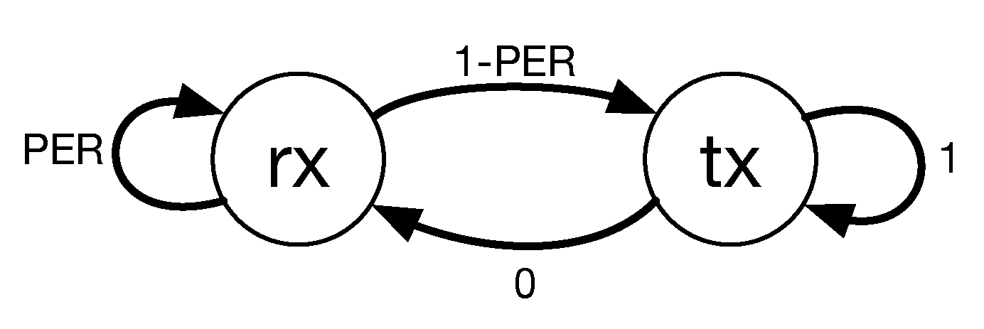
If NONARQ messages with a given number
R of retransmissions are enabled in the network, it may have a significant impact on the network’s reliability. Under this assumption, the retransmission process can be modeled as a one-way Markov model (
Figure 6). A simple transition matrix
P Equation (
7) is straightforward to obtain taking into account Equation (
6) and
Figure 6.
Finally, the Packet Loss Rate (PLR) can be expressed as shows Equation (
8), following the previous matrix notation.
5.3. Integration with Server Software
The developed
software-in-loop platform takes into account the designed software architecture (
Figure 4), which is deeply integrated with the interface module into the server software of the node.
Analyzing the node’s transceiver hardware, there are transmission start/end and reception start/end events, which now have to be simulated. The simulator must keep track of the transmission/reception status of each node to properly simulate their associated hardware. In other words, the simulator has to know what would be the implemented physical modem, which in this work will be CML Microcircuits modem as it is aforementioned. The physical layer bit rate configuration of the system is 1200 bps.
Communication between simulator and server software is performed through a TCP/IP socket. It is encapsulated in packets which carry the associated commands in their payload. The most important and more used command is the transmission request. There are also other commands to control the parameters of the simulated hardware, such as frequency change and transmission power change, but any of these are used in this work.
6. Methodology
In order to demonstrate the feasibility of the software-in-loop approach for simulating a real-time STANAG 5066 protocol stack in underwater RF applications, a set of experiments was carried out. The following subsections introduce the experimental setup and the processes carried out to obtain significant metrics for evaluating the suitability of the platform described in this work.
6.1. Experimental Setup
Two different scenarios were defined in order to assess the impact of the Packet Injection Rate (PIR) and node distance on BER, PLR, and End-to-end delay.
6.1.1. Scenario 1
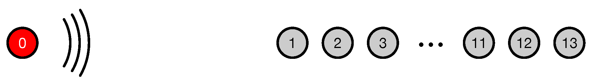
This scenario was defined to perform a simulation of PER and BER and its evolution depending on the distance between transmitter and receiver. For these tests, 14 nodes were set, all of them placed along a straight line (
Figure 7). The first node (Node 0) was placed on the origin of this virtual line, and the other 13 were uniformly placed between 19.5 and 21.5 m. No nodes were placed beyond 21.5 because taking into account Equation (
6) and the propagation model of Equation (
3), the theoretical PLR would be close to 1 beyond that point.
All the nodes were assumed to use 2-FSK modems. Node 0 was configured to use 33 dBm of transmitting power and 116 bytes of packet size, whose 16 first bytes were STANAG 5066 overhead. All application packets carry exactly 100 bytes of payload, so no fragmentation was needed and packets were always of the same length.
As aforementioned, the channel propagation model and the node transmission power leads to find the PER curve interest range between 20.0 and 21.0 m. Therefore, most nodes were placed among these distances, except for the two boundary nodes. The node-placement scheme can be observed in
Table 3.
6.1.2. Scenario 2
This scenario considers the same output powers and modems as Scenario 1, and was specifically designed to carry out experiments involving different PIR. The topology comprises 10 nodes placed along a straight line, equally spaced within a range of 15 m. As a consequence, each node has only communication with its nearest neighbors as depicted in
Figure 8. Node 0 acts as sink, and all the generated traffic has this node as final destination. All the other nodes (from 1 to 9) behave as periodic message generators (with a configurable PIR) and also will route messages from further nodes in order to reach Node 0.
A summary of the simulation parameters, describing physical and STANAG 5066 parameters is shown in
Table 4.
6.2. Description of the Experiments
For the two scenarios mentioned above, three experimental evaluations were carried out. Scenario 1 was used to evaluate the impact of distance and STANAG 5066 ARQ configuration on PLR. On the other hand, Scenario 2 was subject to a long simulation in which a detailed log file was obtained in order to estimate PLR and latency respect to PIR.
6.2.1. Scenario 1
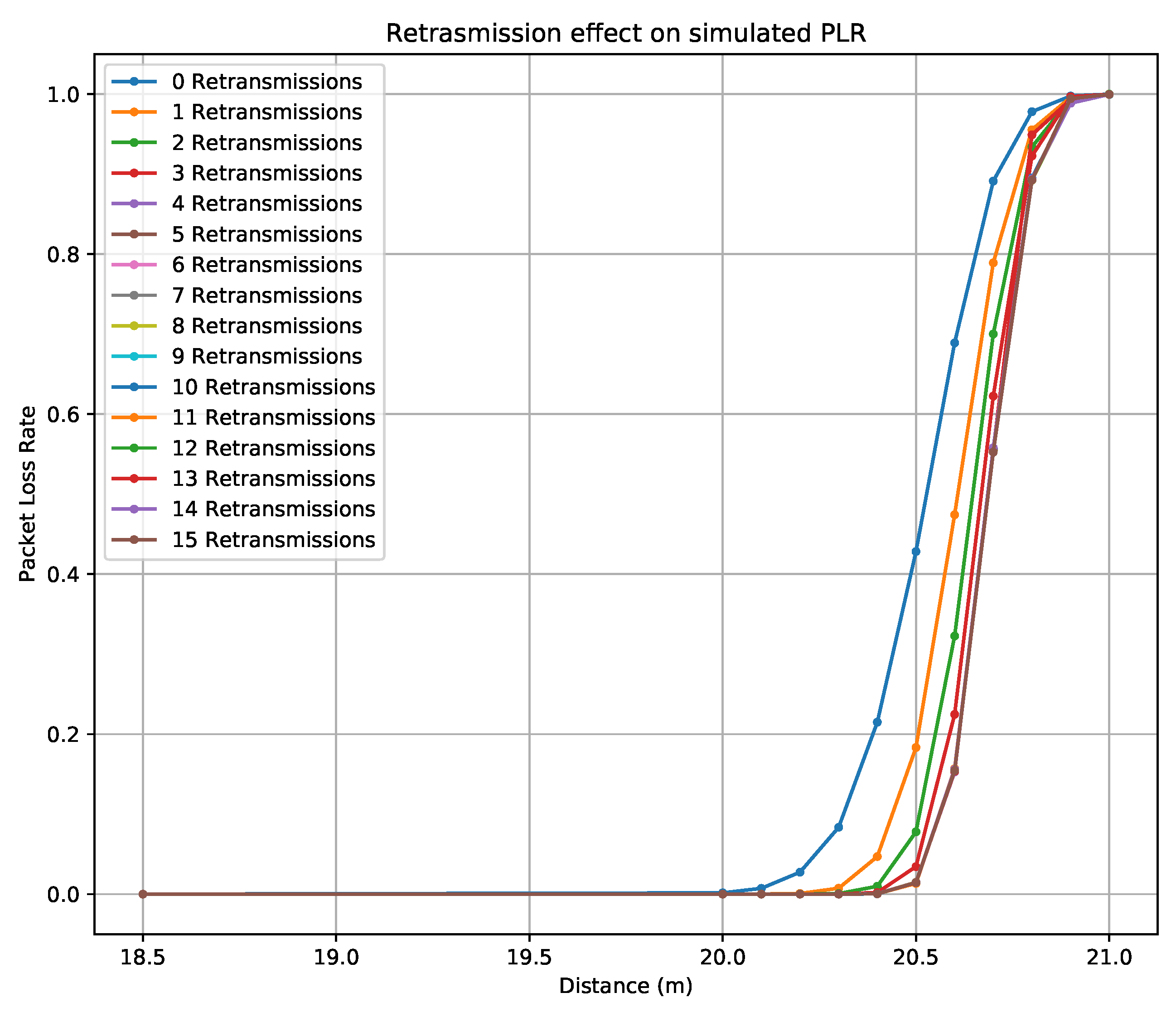
In this case, Node 0 sent a NONARQ message every 20 s. Each message contained a unique ID and a timestamp. The receiver nodes (from 1 to 13) had a passive role, and they only tracked record of all the error-free messages they received. In this scenario, 16 different retransmission configurations were evaluated (from 0 to 15). All the configurations were run independently but simultaneously during enough time to generate a sufficient number of packets. In this case, the simulation was carried out during 25 days, generating more than 110.000 messages.
Transmitter (Node 0) and receiver nodes (from 1 to 13) saved to log files the generated or received messages, containing the aforementioned unique ID for each packet. Each ID generated on Node 0 found on the i-th receiver node incremented a counter, easing the calculation of the PLR as the ratio between found IDs and generated IDs. Finally, thanks to the topology design of this scenario, the PLR of each node corresponded to a link range of interest.
6.2.2. Scenario 2
The objective of Scenario 2’s experiments was to assess the network behavior of a linear topology in terms of latency and PLR. The experimental evaluation of this topology, subject to different values of PIR, would validate the software-in-loop approach developed in this work.
For measuring both PLR and latency, each transmitter node (from 1 to 9) wrote to a log file the information associated to every packet it generated. This information included a timestamp and a unique packet ID. Since that information was included into the packet payload, it could be retrieved at the receiver side, and ultimately written into a reception log. All transmitters’ and receivers’ logs were compared after the execution of the scenario finished. PLR was calculated as in Scenario 1, taking into account that all messages were intended to reach Node 0. Moreover, latency or end-to-end delay was estimated considering the packet-embedded timestamp. It must be taken into account that all the nodes share a common OS clock reference, since the emulated STANAG 5066 stacks are independent processes of the same machine. If a multi-computer simulation approach had been used instead of concurrent execution, the latency would have been impossible to measure, and round-trip time would have substituted it, since no synchronization is needed between nodes.
Different simulations were run to test how the network behaved subject to different values of PIR. For each value of PIR, every node generated packets with a period , with L the network cardinality.
For all the simulations using this scenario, STANAG 5066 ARQ service was used. This means that a STANAG 5066 link is necessary to be created for packet transmissions between nodes. STANAG 5066 link is a handshaking mechanism in which STANAG 5066 standard ensures that the destination node is available to receive data. An initial message was sent from Node 9 to Node 0 prior to start the simulation itself. This strategy ensures that all the links are properly established before generating traffic. The daisy-chain network configuration will make this initial packet to pass through all the nodes of the network, forcing the creation of STANAG 5066 links among neighbour nodes.
Table 5 summarizes the used PIR values and their corresponding
. For each PIR configuration, the simulator ran for 48 h. The total amount of handled packets is also specified in the table.
7. Results
The
software-in-loop platform was running simulations for several days in order to extract the results presented in this section. The log files of all the nodes for all the considered configurations were analyzed using the methodology described in
Section 6. In first place, the results of Scenario 1, which focus on illustrating the impact of distance on each link, are presented. Based on these outcomes, the results of Scenario 2 are comprehensively outlined.
7.1. Impact of Distance
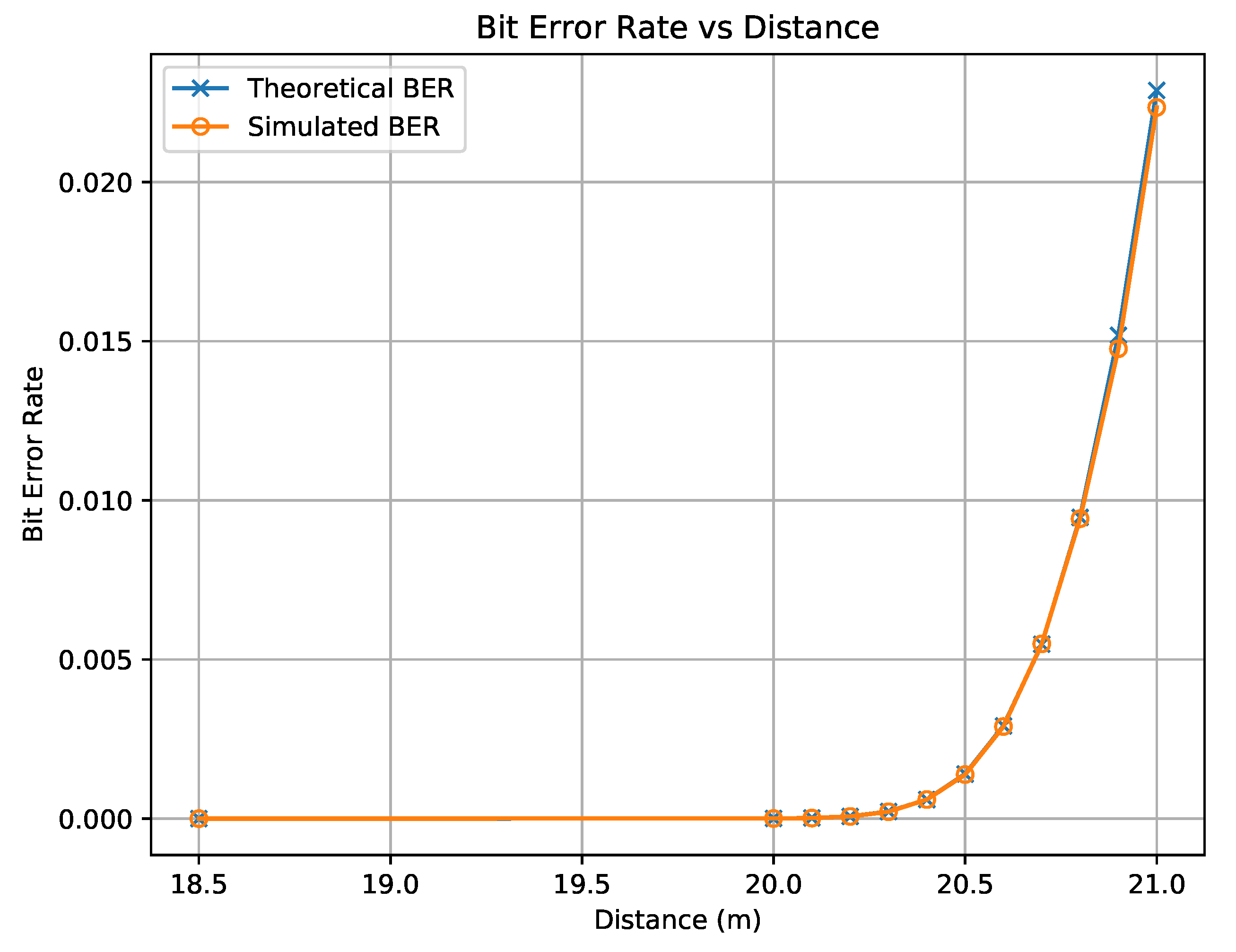
Using Scenario 1’s configuration, the BER curve of a link with respect to distance was obtained.
Figure 9 depicts both the theoretical and simulated curves, which are very close as expected. Similarly,
Figure 10 illustrates the impact of distance on PLR. It can be observed that the number of retransmissions improves the link reliability almost up to 0.5 m with the current physical layer configuration. Furthermore, as it was commented during
Section 6, the maximum achievable link range is below 21 m.
7.2. Impact of Packet Injection Rate
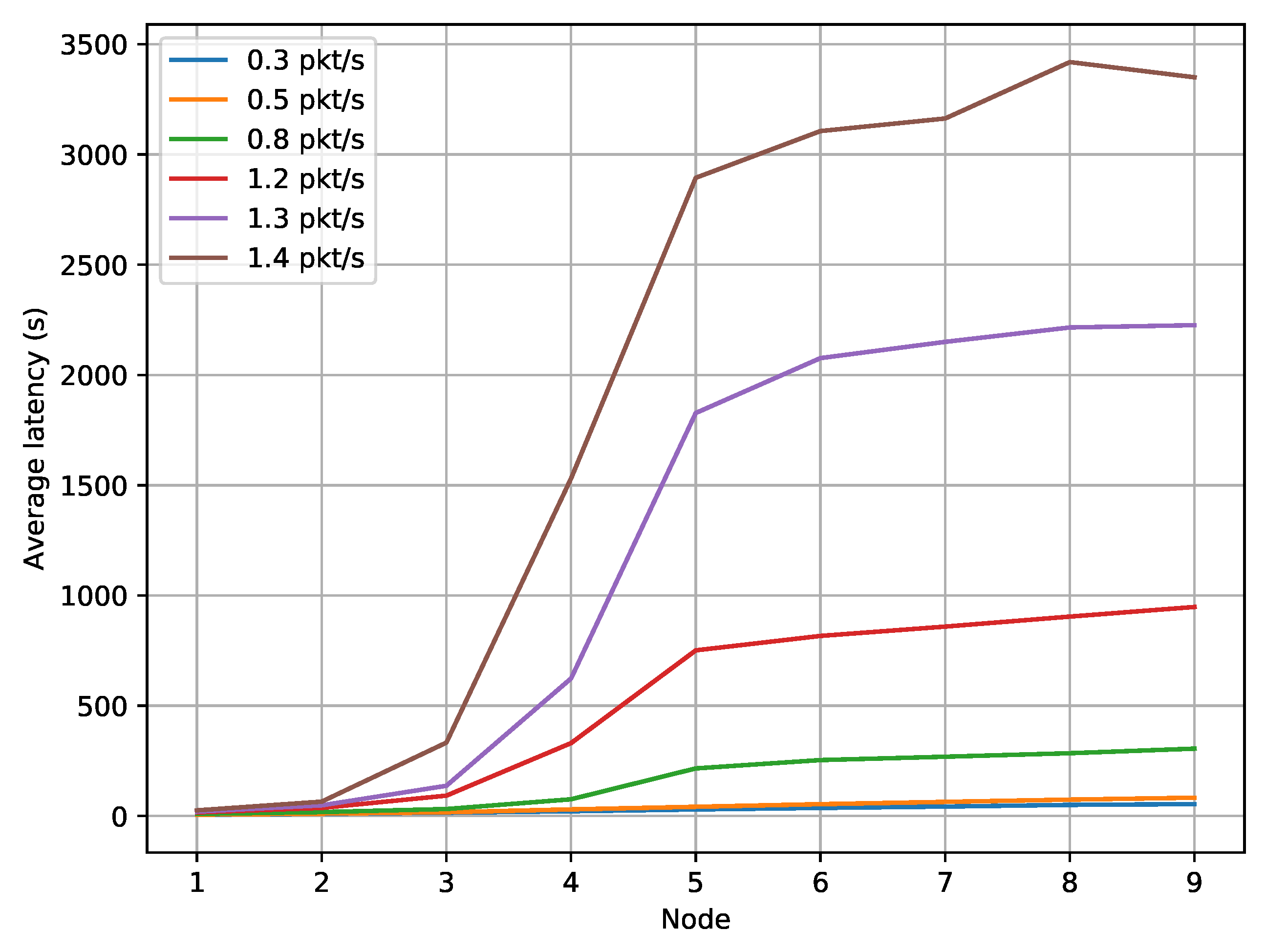
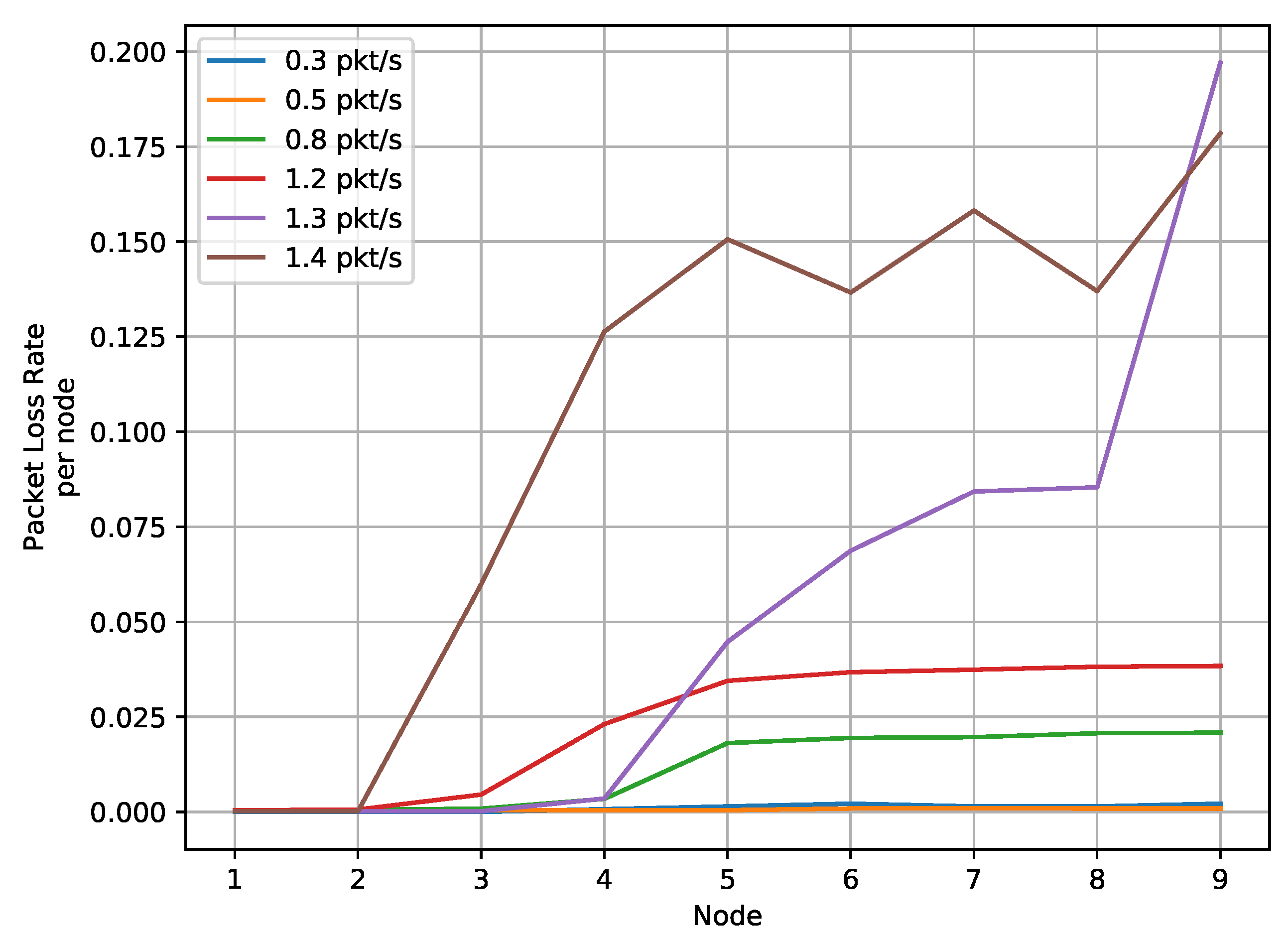
PIR is a parameter that has a huge impact on network performance. It defines the threshold between traffic saturation and smooth packet delivery. The linear design of Scenario 2 will produce a traffic accumulation gradient, forcing the nodes closer to the sink node (Node 0) to make use of the channel more frequently. This effect can be observed in
Figure 11, showing that the farther the node, the higher the latency. The traffic relayed to the following node must be allocated joint to the self-generated traffic. In addition, collisions due to the simultaneous reception of ACK and ARQ messages from neighbouring nodes may induce packet errors. This effect is shown in
Figure 12.
As observed, PLR is also greatly affected by PIR. The same saturation events that caused the latency increase, affected PLR as well. The increment of packet handling while nodes are closer to Node 0 increases transmission times, and this produces a higher number of collisions. STANAG 5066 ARQ protocol implements selective retransmissions, but after a certain amount of time ARQ link is declared as broken, and all the messages buffered by STANAG 5066 stack are discarded. STANAG 5066 informs the upper layer about packet discard, but does not perform any action in this regard. The effect of PIR is more noticeable on those nodes which are closer to Node 0 since they accumulate more traffic, as expected.
8. Discussion
This work has presented a simulation tool capable of real-time simulating an EM-UWSN whilst running production-stage protocol stacks in each of the virtual nodes. The execution of the exact protocol that will be embedded into HERAKLES project’s MINIONs allows an easy evaluation of the expected performance. Furthermore, the developed simulator interacts with the STANAG 5066 stack at byte level, treating the software piece under evaluation as a black box. This approach has many advantages from a practical viewpoint. For instance, the orchestration of the network simulation is reduced to controlling message delivery, since each real-world STANAG 5066 stack is carrying out MAC and PHY operations on their own. In addition, the simulated nodes can execute exactly the same routines that will perform under real operation (apart from STANAG 5066). Finally, the presented framework eliminates the necessity of designing the code taking into account specific API constraints, as it occurs with Click or UnetStack.
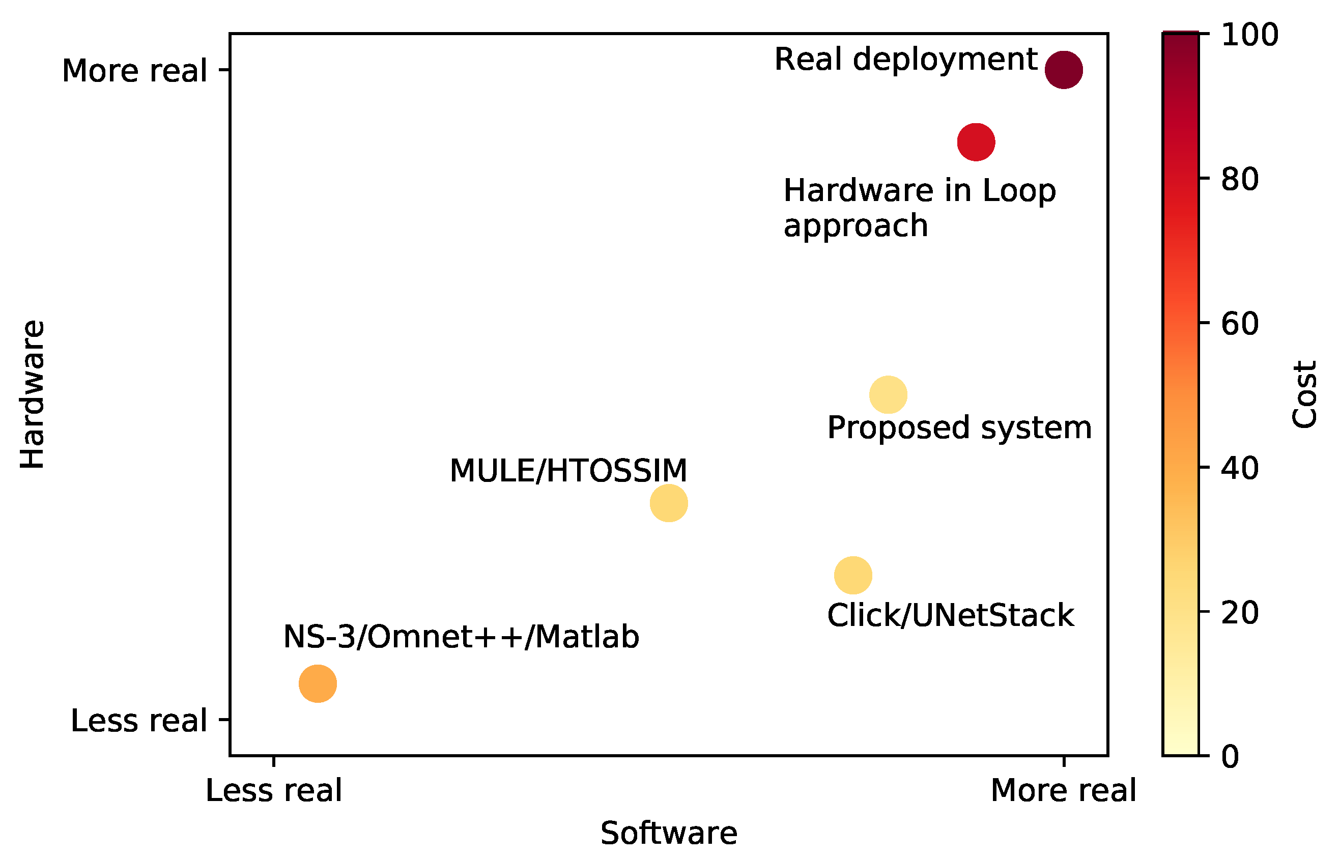
Figure 13 illustrates a comparison relating the realism and cost of different network simulation approaches. The more realistic both software and hardware are, the more expensive the schemes turn. Hardware-in-loop is closer to an actual deployment as it pretends to use the same hardware with minor modifications, with the purpose of adapting it to the simulation hardware. On the other hand, DES (OMNET++, NS-3, MATLAB, etcetera) needs a protocol implementation compliant with the simulation framework’s constraints. Generally, simulating using DES is more unrealistic, but is cheaper and faster. Finally, hybrid simulation (MULE, HTOSSIM) and the use of SCL (such as Click or UnetStack) are more software-realistic, but the development cost is higher since the implementation must fit within the framework’s API.
The simulated network scenario corresponds to a linear deployment in which each node has only visibility with its neighbours. Furthermore, all the nodes generate traffic depending on a network parameter (PIR). Although the scenario’s topology is relatively simple and the distance between nodes minimizes PER, the results suggest that there is a significant amount of collisions. As it was commented in
Section 3, if after waiting the corresponding initial back-off time a node determines that the channel is idle (from its viewpoint, obviously), it carries out the transmission of all the queued messages up to 60 s. Taking into account the parameters of
Table 4, this means that a maximum of 77 queued messages can be transmitted each time. However, since each node is unable the sense transmissions of nodes located above a single-hop distance, collisions are likely to happen. This fact, joint to the long transmission times would make that sometimes a link should be marked as broken. This breakage directly implies that all the buffers are flushed, and hence this information is lost (ultimately increasing PLR). The obtained simulation results suggest that a PLR below 5% for all the network can be assured for PIR values lower than 1.2 packets per second.
Regarding packet delivery time, it was observed that the traffic accumulation effect of the linear topology had a significant impact. In general terms, the latency of the i-th node
can be expressed in terms of medium access delay (
), transmission delay (
), and queueing delay (
). This relation is shown in Equation (
9).
The values of each delay component are different for each node. In general terms, messages flow from each node to the sink, whilst ACKs perform in the opposite direction but just from the immediately forward node. Hence, the traffic originated in the farthest node, will be subject to a higher collision probability since it must be forwarded several times before reaching the sink node. Considering the 0-th node as the sink node, the delay of a packet (
) generated at the
i-th node will accumulate the latencies of the following relaying nodes as expresses Equation (
10). This effect is clearly observed in
Figure 11, in which higher PIR values induce higher collision probabilities and therefore larger delivery times.
Furthermore, the collision probability depends on the amount of traffic accumulated by each node, since larger buffer usage implies longer transmission times (and therefore channel occupation). The average transmission delay depends on the amount of retransmissions, which is inversely proportional to the collision probability. Moreover, medium access delay also depends on this probability and ultimately affects transmission delay, conforming a complex relationship that is, in addition, different for each node.
Although the obtained results reflect the actual behavior of the STANAG 5066 stack assuming the EM-URFC model presented in
Section 4, by the own definition of the real-time paradigm proposed in this work, simulations cannot be sped up as it occurs in DES. The unitary time scale of the
software-in-loop simulator may affect the design of routing or discovery protocols, due to the potentially-excessive time consumption. Nevertheless, the original motivation of this work was not aligned with network-level protocol design. The main objective of this work was to provide a robust and accurate platform to simulate production-ready protocol stacks (STANAG 5066 in this case) under real-time operation inside arbitrarily complex networks. The obtained results demonstrate that the proposed framework can be used to simulate STANAG 5066-based EM-URFC UWSN (and any other stack and channel with minimum adjustments).
9. Conclusions
In this work, the development of a software-in-loop platform to perform UWSN simulations using a real-time STANAG 5066 stack has been presented. The used STANAG 5066 stack is part of a real-world implementation of an EM-based underwater node, framed within Spanish Government’s project HERAKLES. The main objective of this work was to assess the suitability of this software-in-loop simulation approach.
The developed platform integrated a STANAG 5066 stack, but any real-time implementation of production-stage software could be easily integrated with minor modifications. The configurable time-slicing scheme of the simulator allowed to select the appropriate granularity in order to guarantee the real-time processing whilst maintaining CPU usage below a critical threshold.
Taking into account the particularities of STANAG 5066, the simulated results showed no significant divergence from the expected behavior. Two scenarios were simulated. The first one comprised a broadcast situation that was used to assess the performance of NONARQ retransmissions. It was observed that including this feature could improve the effective link range about 0.5 m (using the simulation parameters of
Table 4). Moreover, the results on Scenario 1 demonstrated that the integration of STANAG 5066 communications stack with the developed platform did not show any type of bottleneck. On the other scenario, in which a linear UWSN was deployed, the impact of PIR on both latency and PLR was evaluated. The results suggested that PIR has a critical impact on both parameters, showing a behavior that is within the limits of the expected one. As the PIR increased, the bottleneck link due to traffic accumulation was easily identified. In addition, latency dramatically increased with PIR for the farthest nodes.
This work has demonstrated many advantages in terms of the evaluation of real protocol stack implementations. Furthermore, the physical layer has been simulated using a model based on real-world measurements, but it does not take into account other phenomena such as fading or complex channel impulse responses. Nonetheless, the simulation platform could be improved by integrating the aforementioned physical phenomena in the channel propagation software block.
This work has demonstrated through simulation that software-in-loop techniques are feasible for EM-UWSN using STANAG 5066. The obtained outcomes will be used in further works to simulate real-world deployments using HERAKLES’ underwater nodes.


