1. Introduction
Technical literature concerning three-phase motor drive systems is very wide and rich in contributions investigating several aspects related to that kind of systems. A first set of contributions is related to functional issues such as, for example, the control strategies for three-phase inverters (e.g., [
1]). A second set of contributions is related to circuit modeling and measurement techniques of conducted electromagnetic interference (EMI) [
2,
3,
4,
5,
6,
7,
8,
9,
10,
11,
12]. This point is crucial in modern power systems due to the widespread and pervasive use of power electronics. EMI modeling, indeed, is essential for both analysis and EMI mitigation techniques.
As far as the EMI issue is considered, several approaches have been used to model the high-frequency behavior of power converters. Time-domain and frequency-domain approaches have both several disadvantages, such as long computational time and system oversimplification, respectively. Such drawbacks are potentially overcome by a further approach consisting in the behavioral modeling of power converters, based on the extraction of Thevenin or Norton equivalents from EMI measurements [
6].
In all the approaches mentioned above, conducted EMI are modeled as the superposition of differential-mode (DM) and common-mode (CM) noise. Such separation is essential in EMI modeling and filter design [
13,
14,
15,
16,
17,
18]. It is well-known; however, that such sharp separation between DM and CM noise is possible only under the assumption that the converter is perfectly symmetrical with respect to the ground. In fact, system asymmetries lead to DM–CM noise transformation (i.e., noise conversion between the two noise components) [
6,
19].
Several papers can be found about this point when single-phase converters are considered [
19,
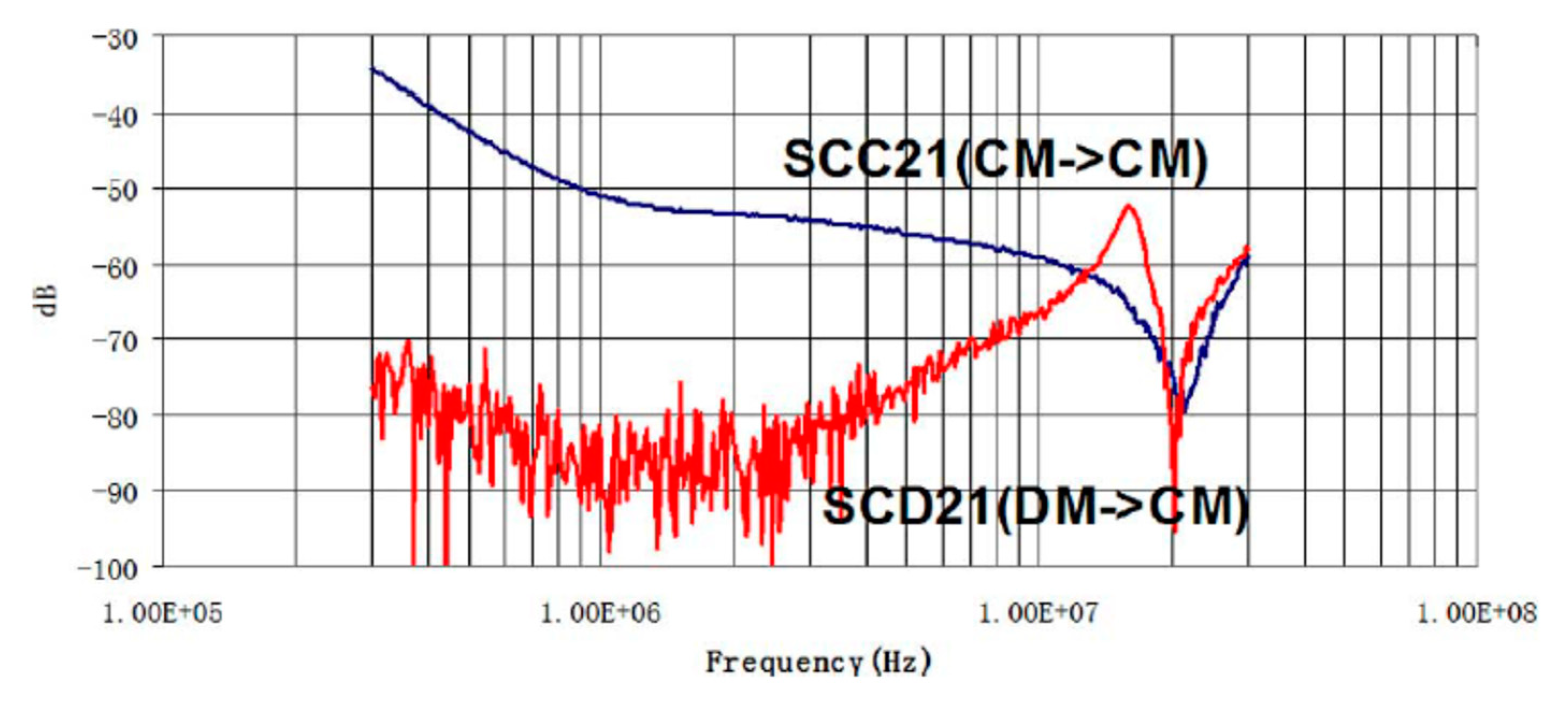
20]. As an example,
Figure 1 shows measured DM–CM noise transformation due to asymmetries in an EMI filter [
19]. As far as three-phase converters are studied, however, few analytical contributions are available in the literature. Nevertheless, mode conversion in three-phase converters is well documented by experiments. For example, the experimental results reported in [
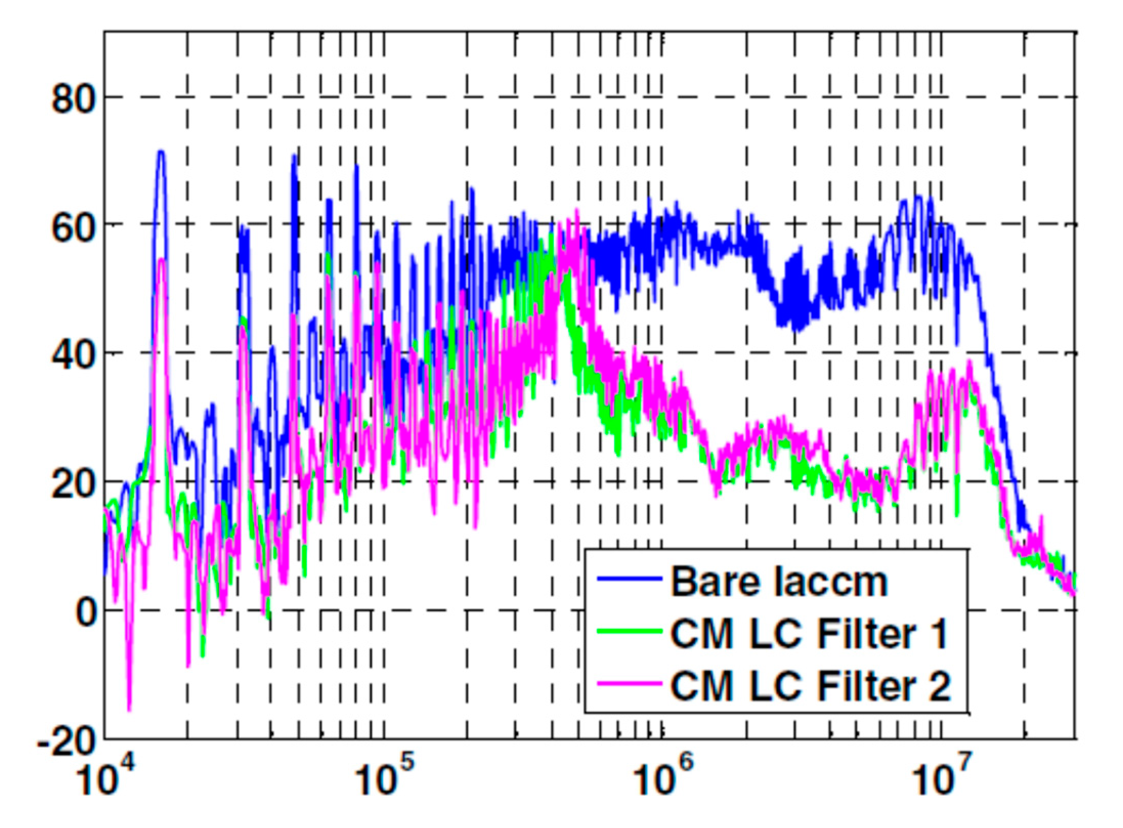
21] show clearly that the three-phase LC filter is a critical component. In fact, in case of slight filter asymmetry, the DM resonances can be measured as resonances in the CM current. As an example,
Figure 2 shows the amplitude spectrum of the measured CM current in the three-phase motor drive system reported in [
21]. The blue curve was measured without filter, whereas the green and the magenta curves were measured for two different values of the DM inductances (i.e., 3.5 and 2.5 μH, respectively) of a DM–CM LC filter. The resonances of the DM circuit (i.e., 380 and 450 kHz corresponding to the two values of the DM inductance, and 50 nF capacitance) were clearly measured in the spectrum of the CM current. This is a clear experimental evidence of DM-to-CM noise conversion. Recognizing this point is crucial for a proper filter design. In fact, if DM-to-CM noise conversion is not recognized, unnecessary overdesign of the CM filter could be implemented.
Although the general idea of noise mode conversion due to three-phase asymmetry is well established, to the Author’s knowledge a rigorous analytical description of differential-to-common-mode noise conversion in three-phase systems is still a challenging point. The main novelty introduced in this paper is the mathematical derivation and explanation of differential-to-common-mode noise transformation in asymmetrical three-phase systems by resorting to the Clarke transformation and the eigenvalue analysis. In particular, differential-to-common-mode noise conversion due to a slightly asymmetrical LC filter will be investigated. The proposed methodology, however, has general validity. Thus, the analytical results derived in the paper can be used to describe the impact on the CM circuit of any three-phase asymmetry (e.g., asymmetrical cable parameters). It will be shown that, in case of three-phase asymmetry, the CM circuit is affected by the DM circuit on the whole frequency axis, but the main impact is due to the DM resonances injected into the CM circuit. Thus, the spectral lines corresponding to the DM resonances appear in the amplitude spectrum of the CM current with shifted frequency. The proposed analytical derivations provide the magnitude and the frequency location of the CM current peaks due to noise conversion, as functions of the filter asymmetry.
A second novelty introduced in the paper is a statistical analysis based on the assumption that, due to component tolerances, the filter parameters can be treated as random variables. Randomness in the filter parameters results in randomness in the frequency location of the CM current peaks due to differential-to-common-mode noise conversion. A complete statistical characterization of the frequency shift of the CM current peaks due to noise conversion is derived in terms of probability density function, mean value, and variance.
The relevance of the analytical results derived in the paper can be summarized in two points. First, the differential-to-common-mode noise conversion in an asymmetrical three-phase system is rigorously described in terms of theoretical properties and circuit equivalents. Second, the derived models allow quantitative prediction and explanation of the impact of noise conversion on frequency-domain measurements of CM currents.
The paper is organized as follows. In
Section 2 the Clarke transformation is recalled, and its relationship with the well-known symmetrical component transformation in the frequency-domain is clarified. In
Section 3 the impact of asymmetrical parameters of the LC filter on the differential-to-common-mode noise conversion in a three-phase motor drive system is described in analytical terms. To this aim, the equations in terms of Clarke variables are decoupled through the eigenvalue analysis. The magnitude and frequency location of the CM current spectral lines due to DM resonances are provided in closed form. In
Section 4, specific three-phase motor drive system is implemented in Simulink to provide numerical validation of the analytical results.
Section 5 is devoted to the statistical analysis of differential-to-common-mode noise conversion. In particular, by treating the asymmetrical parameters of the LC filter as random variables, the probability density function, the mean value, and the standard deviation of the frequency location of the CM current peaks from noise conversion are derived in closed form. Finally, conclusions are drawn in
Section 6.
2. The Clarke Transformation
The analytical derivations proposed in the next Sections are based on the well-known Clarke transformation, which is a mathematical transformation broadly used in the analysis of three-phase power converters [
22]. In fact, under the common assumption of circuit symmetry between the three phases, the Clarke transformation allows the introduction of voltage/current space vectors able to provide a compact and meaningful description of the three-phase system.
The Clarke transformation operates on a triplet
a,
b,
c, of time-domain phase variables (e.g., phase voltages and currents) to obtain a triplet of transformed variables named
α,
β, and 0. For example, by considering phase currents, the Clarke transformation operates as:
It is worth noticing that the transformation defined in (1) is in its rational form (i.e., the transformation matrix T is orthogonal ()). This property guarantees power conservation across the transformation and allows consistent derivation of equivalent circuits in the transformed domain.
In case of circuit symmetry between the three phases, the transformation matrix
T operates diagonalization of parameter matrices. For example, by considering the inductance matrix
L of a three-phase component with symmetrical phases:
Similar results can be obtained for capacitance/resistance matrices. Matrix diagonalization is a crucial point since it results in decoupled equations in the transformed variables. Notice that
α and
β parameters in the transformed matrix take the same values (i.e.,
in (2)). This means that the
α and
β equations have the same structure and the same parameters. Therefore, the
α and
β circuits can be treated as a single circuit with the
α and
β variables combined to form complex space vectors. Each space vector has a real part given by the
α component and imaginary part given by the
β component. Thus, the current space vector corresponding to (1) is defined as:
where
. Notice that since the Clarke transformation operates in the time domain, it can be used to analyze three-phase systems under transient conditions. However, when distorted steady-state conditions are considered, the same transformation in (1) operates on the phasor quantities at each frequency. In this case, the Clarke transformation can be put in relation with the well-known symmetrical component transformation [
23]. The following relationship between phasors can be readily derived:
where
,
, and
are the positive, negative, and zero-sequence phasor components, respectively. Notice that from (4) we obtain that the
α component is proportional to the sum of the positive-sequence and negative-sequence components, whereas the
β component is proportional to the difference between the same quantities. The zero-component
of the Clarke transformation equals the zero-sequence component
. Thus, the
α and
β components can be identified as the common mode (CM) and the differential mode (DM) of the pure three-phase system, respectively, whereas the zero-component can be identified as the conventional CM resulting from the interconnection of a three-phase circuit with a single-phase circuit. That is the usual condition of a three-phase inverter where the so-called CM current circulates in a single-phase circuit consisting mainly in the system parasitic elements.
Finally, it is worth highlighting that the diagonalization property (2) of the Clarke transformation holds only in case of circuit symmetry between the three phases. In case of asymmetrical phases, the straightforward use of (2) leads to a full matrix (i.e., to circuit coupling between the Clarke variables
α,
β, 0) [
24]. In particular, since the zero components correspond to the conventional CM variables, asymmetrical phases result in injection of
α and
β component currents into the CM circuit. The theoretical investigation of such phenomenon is presented in the next Sections where the spectral lines of the CM current due to phase asymmetry are characterized in analytical and statistical terms.
3. Differential-to-Common-Mode Conversion Due to LC Filter Asymmetry
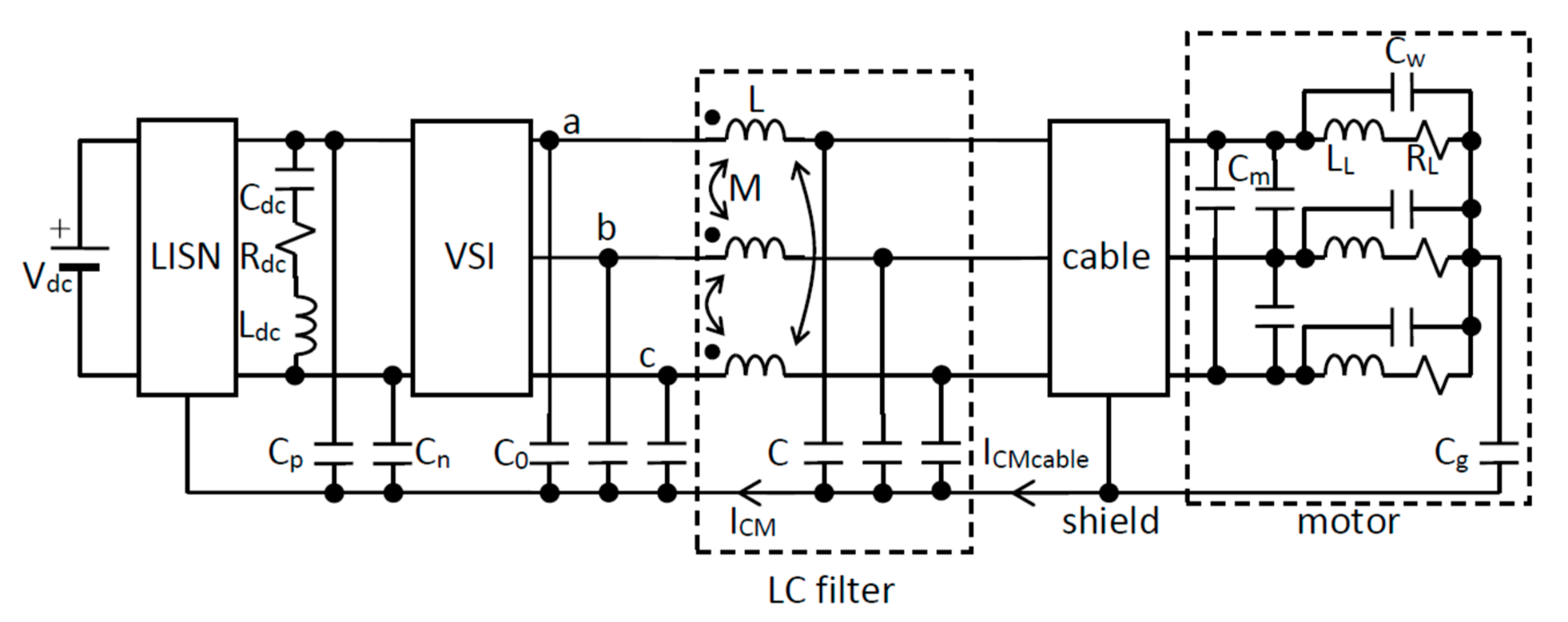
Let us consider the three-phase motor drive system represented in
Figure 3 and consisting in a dc-fed three-phase inverter, a line impedance stabilization network (LISN), a dc-link capacitor, a CM/DM LC filter, a shielded cable, and an induction motor. The LC filter is realized by means of a CM choke whose leakage inductance provides DM filtering, and three star-connected grounded capacitors [
21]. The following derivations, however, have general validity and can be readily adapted to different filter realizations. The cable is represented by a lumped RLC circuit, whereas each motor phase is represented by a series RL connection and a parallel capacitor to take into account high-frequency effects of windings.
The main parasitic elements are also included in the model, that is, the series resistance and inductance of the link capacitor , the capacitances and from the dc-bus to the ground, the three capacitances from each inverter phase to the ground, the motor input capacitances , and the capacitance between motor windings and frame.
The following analysis considers the impact of asymmetrical values of the LC filter parameters on the differential-to-common-mode noise conversion. The proposed methodology, however, can be readily used to investigate the impact on noise conversion of other asymmetrical parameters (e.g., the three-phase cable parameters).
3.1. Circuit Modeling and Analytical Derivations
The three-phase system depicted in
Figure 3 can be analyzed through the Clarke transformation recalled in
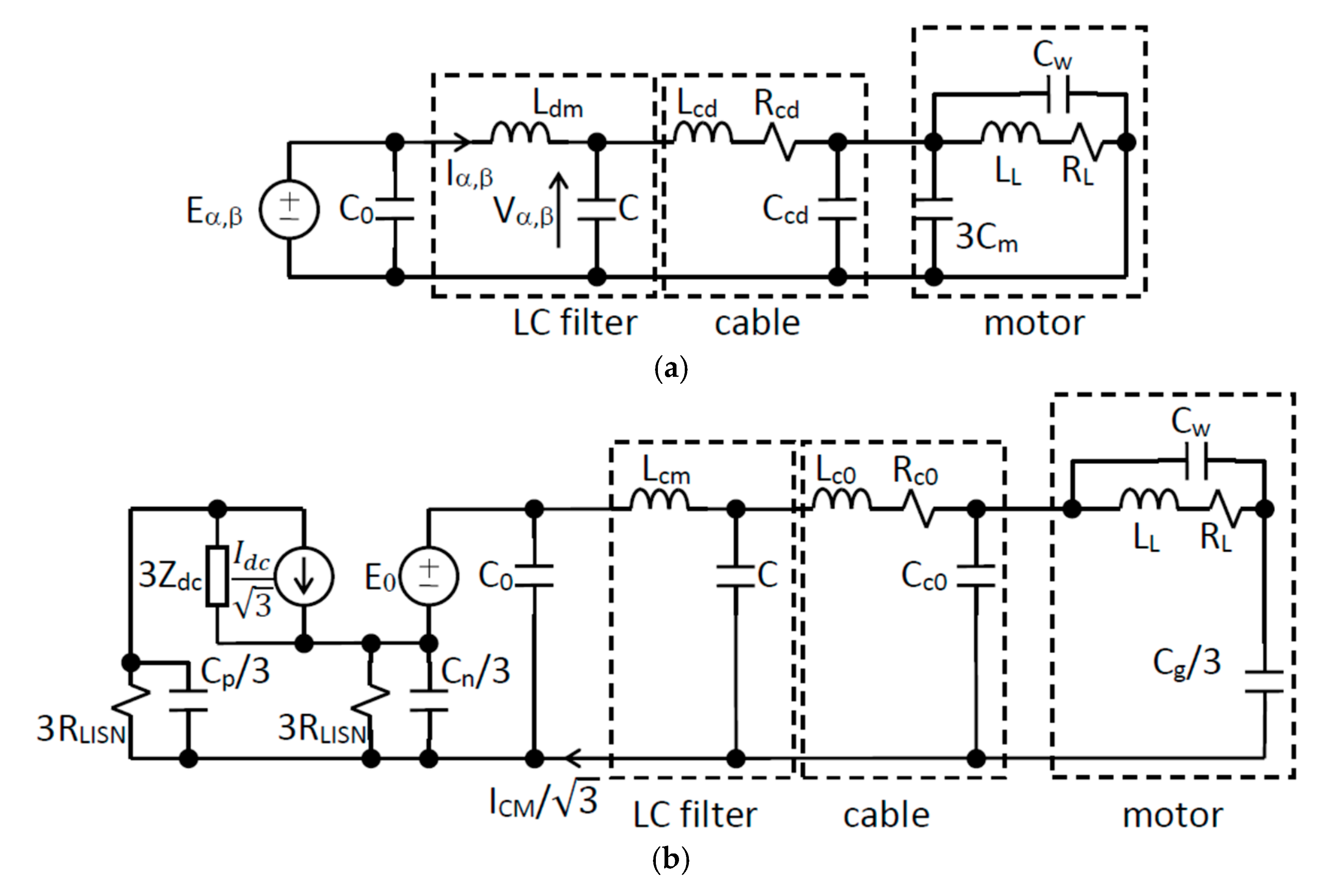
Section 2. In case of ideal circuit symmetry between the three phases, the
α and
β circuits show the same topology and the same parameter values (see
Figure 4a). To this aim it is worth recalling that the topology of
α and
β circuits follows the same rules as the positive- and negative-sequence circuits for the symmetrical components, that is, a short circuit connects all the star centers of the three-phase system (notice that the delta-connected capacitors
can be first transformed into star connected capacitors
) [
23]. As far as the zero-component circuit is considered, however, a different circuit topology is obtained (see
Figure 4b). In fact, by following the same rules valid for the zero-sequence component in the symmetrical components framework, the interaction between the three-phase and the single-phase parts of the system must be taken into account. In particular, in previous works it was shown that a single-phase circuit connected to the star centers of a three-phase circuit can be moved, with unchanged topology, to the three-phase side through a multiplication by 3 of single-phase impedances and by
of single-phase voltage sources, and division by
of single-phase current sources [
23,
24].
In case of circuit symmetry between the three phases, the α, β, and zero circuits are uncoupled. In particular, the resonances of the α and β circuits have no impact on the zero circuit. It can be easily observed that the main resonance in the α and β circuits is given by the filter components. In fact, the low-level impedance corresponding to the large filter capacitance is only slightly affected by the high-level cable and motor impedances due to capacitances much smaller than . Thus, the differential-mode inductance of the filter can be approximately considered in series with the filter capacitance . The resulting series resonance is located at the frequency . In case of asymmetrical filter components, it is expected that such resonance is injected into the zero-component circuit (i.e., the CM circuit). The impact of asymmetry in filter capacitances and inductances on the CM circuit is analyzed in the following Subsections.
3.1.1. Asymmetrical Filter Capacitors
As far as the filter capacitors
are considered, the simple case of a small perturbation
of the capacitance connected to the phase
a is first investigated. The voltage–current relationship for the phasor Clarke components is given by [
25]:
After simple algebra the following equations can be obtained from (5):
where it is apparent that the
β circuit is not affected by the capacitance perturbation.
The interaction between
α and 0 circuits can be investigated by introducing two reasonable approximations in (6a) and (6c). First, under normal conditions the zero-component variables are much smaller than the
α and
β variables. Moreover, the impact of
α and
β circuits on the zero-component circuit is large around the resonances of
α and
β circuits. Therefore, in (6a) it is reasonable to assume
(i.e., no feedback is assumed from the zero to the α circuit). Second, the small perturbation assumption
allows for neglecting the term
in (6c). Therefore, the approximate versions of (6a)–(6c) are given by:
From (7a) we observe that the equivalent α capacitance is changed by the additive term
. As a consequence, the resonance in the α circuit is shifted to the value
Such resonance has impact on the zero-component circuit through (7c):
Thus, the resonance in the α circuit is injected into the CM circuit. The frequency location of the corresponding spectral line is given by (8), and both the frequency location shift and the magnitude of the spectral line are proportional to the capacitance deviation .
The above analytical results hold in the case of capacitance deviation of the phase a. It is expected that similar results hold in case the capacitance deviation is placed on the phase b or c. By writing (5) for or , however, the equations corresponding to (6a)–(6c) do not allow a straightforward interpretation as in the case of because a further coupling is introduced between α and β variables. Moreover, from both theoretical and practical viewpoint, the general case of simultaneous deviation of all the three parameters , , and would be of interest. To this aim, a more general analytical approach is derived.
In case of simultaneous deviation of the three capacitances with respect to the nominal value
, the Clarke transformation:
provides the three equations:
By introducing the same approximation used above (i.e., negligible feedback from the zero-component circuit to the
α and
β circuits), for the
α and
β variables we obtain the following approximate expressions:
Therefore, the problem can be reformulated as the diagonalization of a matrix:
where:
It can be readily shown that the eigenvalues of
A are given by:
By substituting (15) into (16), after simple algebra we obtain the eigenvalues
of the full matrix in (13):
It is worth noticing that in (17) the term in the first bracket is the mean value of the capacitance deviations, whereas the square-root term represents the root mean square value of the capacitance deviations.
The matrix
P of the eigenvectors, corresponding to the eigenvalues (17), when applied to (13) leads to transformed variables:
and matrix diagonalization:
Therefore, we obtain decoupled equations in the transformed variables:
The fundamental result in (20) provides two different shift values to the nominal capacitance
in case of distinct eigenvalues (17). This means that under the general condition of two or three capacitance deviations, two different resonances are generated in the
α and
β circuits, and they are coupled into the zero-component circuit through (11c). The frequencies of the two resonances are given by:
Notice that in the special case of only one capacitance deviation (i.e., any phase, a, b, or c), one of the two eigenvalues (17) is zero, whereas the second is given by . Null eigenvalue means no circuit interaction (i.e., only the resonance corresponding to is injected into the zero-component circuit). Therefore, only one spectral line due to mode conversion is present in the CM current in case of one capacitance deviation, whereas two spectral lines are expected in case of two or three capacitance deviations.
Finally, in case of equal capacitance deviations from (17), we have one double eigenvalue, but from (11c) there is no interaction with α and β circuits. This is consistent with the fact that means symmetrical capacitance values.
3.1.2. Asymmetrical Filter Inductors
A CM choke can be modeled as a coupled three-phase inductor according to (2). In the symmetrical case the DM inductance is , and the CM inductance . Notice that small asymmetrical self-inductances can result in large relative deviations of the DM inductance , because usually and take close values.
By assuming simultaneous deviations of the three self-inductances with respect to the nominal value
, the Clarke transformation:
provides the following equations:
By introducing the same approximation used in the previous Subsection (i.e., negligible feedback from the zero circuit to the
α and
β circuits), for the
α and
β variables we obtain the following approximate expressions in matrix form:
The full matrix in (24) has the same structure as (14). Therefore, the matrix diagonalization can be obtained by using the same results already shown in
Section 3.1.1. In particular, from (16) we obtain the eigenvalues:
Thus, the corrected values of the inductance in the
α and
β circuits are given by
and
. The corresponding frequencies of the resonances injected into the zero-component circuit are given by:
The same remarks already highlighted for (21) hold for (26). In particular, it is worth noticing that, in general, two spectral lines are generated in the CM circuit, and the frequency displacement with respect to the ideal location depends on .
Finally, the case of asymmetrical mutual inductances
can be included into the above derivations. Starting from the Clarke transformation of a completely asymmetrical inductance matrix:
by simple algebra and by using the approximation of no-feedback from the zero-component circuit to the
α and
β circuits we obtain:
The eigenvalues of the full matrix in (28) can be still evaluated through (16). Explicit expressions are not reported here for the sake of simplicity. Also in this case the eigenvalues result, in general, in two inductance shifts and , and the related resonance frequencies injected into the zero-component circuit.
4. Numerical Validation
The three-phase motor drive system represented in
Figure 3 was implemented in Simulink. The three-phase voltage source inverter (VSI) was controlled with pulse width modulation (PWM) with 50 Hz modulating frequency and 1650 Hz carrier frequency (i.e., the frequency-modulation ratio was 33), whereas the amplitude-modulation ratio
m was 0.95.
was 100 V,
, and the dc-link capacitor was represented by a high-frequency equivalent circuit consisting in the series connection of
,
, and
. The VSI parasitic capacitors were
and
. The LC filter was implemented by a CM choke with
and
, and star-connected capacitors with
[
21]. Thus, the DM and CM cutoff frequencies were
and
, respectively. The shielded cable was represented by a lumped equivalent circuit (see
Figure 4) with
,
,
, and
. Thus, the DM and CM cable resonance frequencies were
and
, respectively. The motor phases were represented by
,
, and
, whereas the motor parasitic capacitances were
and
.
The time-domain simulations were performed with sampling frequency
, and the samples of the CM current (see
Figure 3) were processed through the fast Fourier transform (FFT) to obtain the amplitude spectrum within the
frequency range.
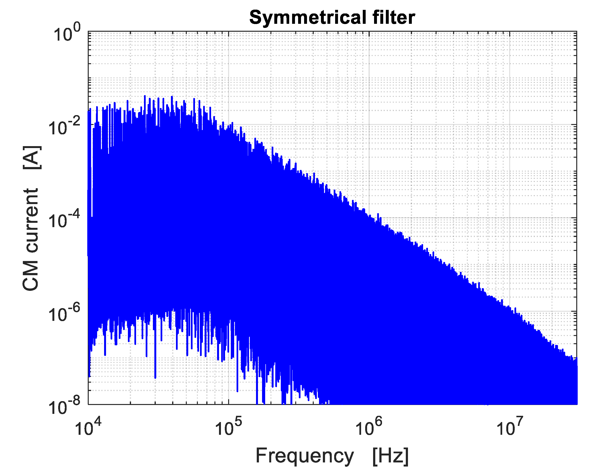
Figure 5 shows the amplitude spectrum of the CM current (limited to
, according to the conducted emissions standards [
21]) in case of filter symmetry. The impact of the CM filter with
cutoff frequency is clearly apparent. Moreover, no resonance frequencies can be identified (i.e., no peaks), even in proximity of the DM resonance located at
. This means that, according to the theory, in case of symmetrical parameters there is no interaction between DM and CM circuits.
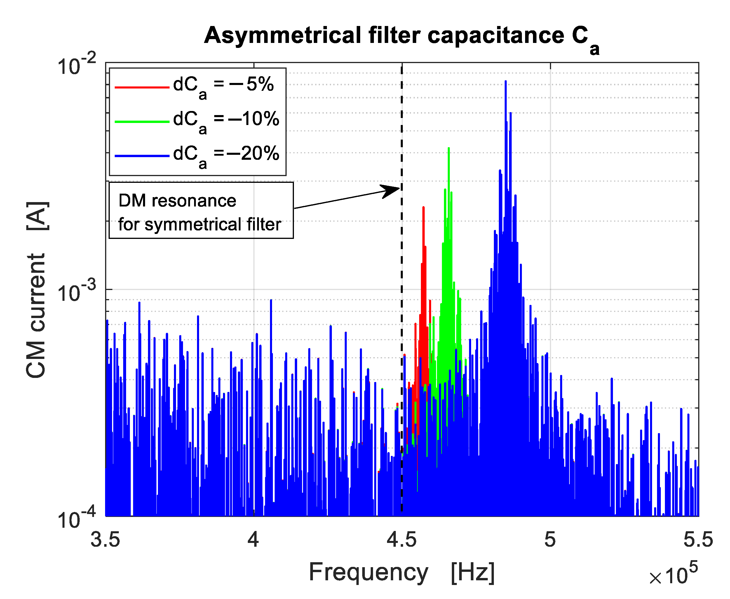
Figure 6 shows the effect of a deviation
of the filter capacitance
with respect to its nominal value
. According to (8), a negative deviation
results in a positive relative increase
in the resonance frequency of the α circuit. Moreover, according to (9) such resonance is injected into the CM circuit with increasing magnitude with the deviation
. This is confirmed in
Figure 6, where three different percent values of
were selected (i.e.,
,
, and
). The corresponding shift in the DM resonance frequency (i.e.,
) are given by
,
, and
, respectively. According to the eigenvalue analysis derived in
Section 3.1.1, similar results can be obtained when the asymmetrical capacitance is either
or
.
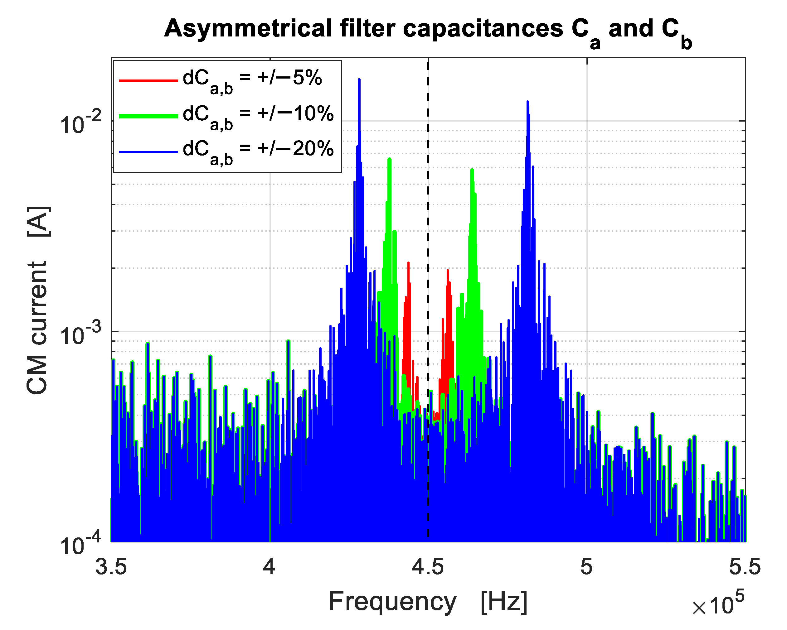
Figure 7 shows the case of two simultaneous deviations
and
. The deviation
was selected such that
. According to (17) and (21), the two eigenvalues are
, and the two resonance frequencies
. Thus, the two peaks have frequency separation
. Three different percent values were assumed for
(i.e.,
,
, and
). The corresponding frequency separation of each couple of peaks are 13 kHz, 26, kHz, and 52 kHz. This point is confirmed by
Figure 7. Notice that for
the two peaks (blue line) are not perfectly symmetrical with respect to
. This is because the formula
is approximate, and it provides better results for small values of
.
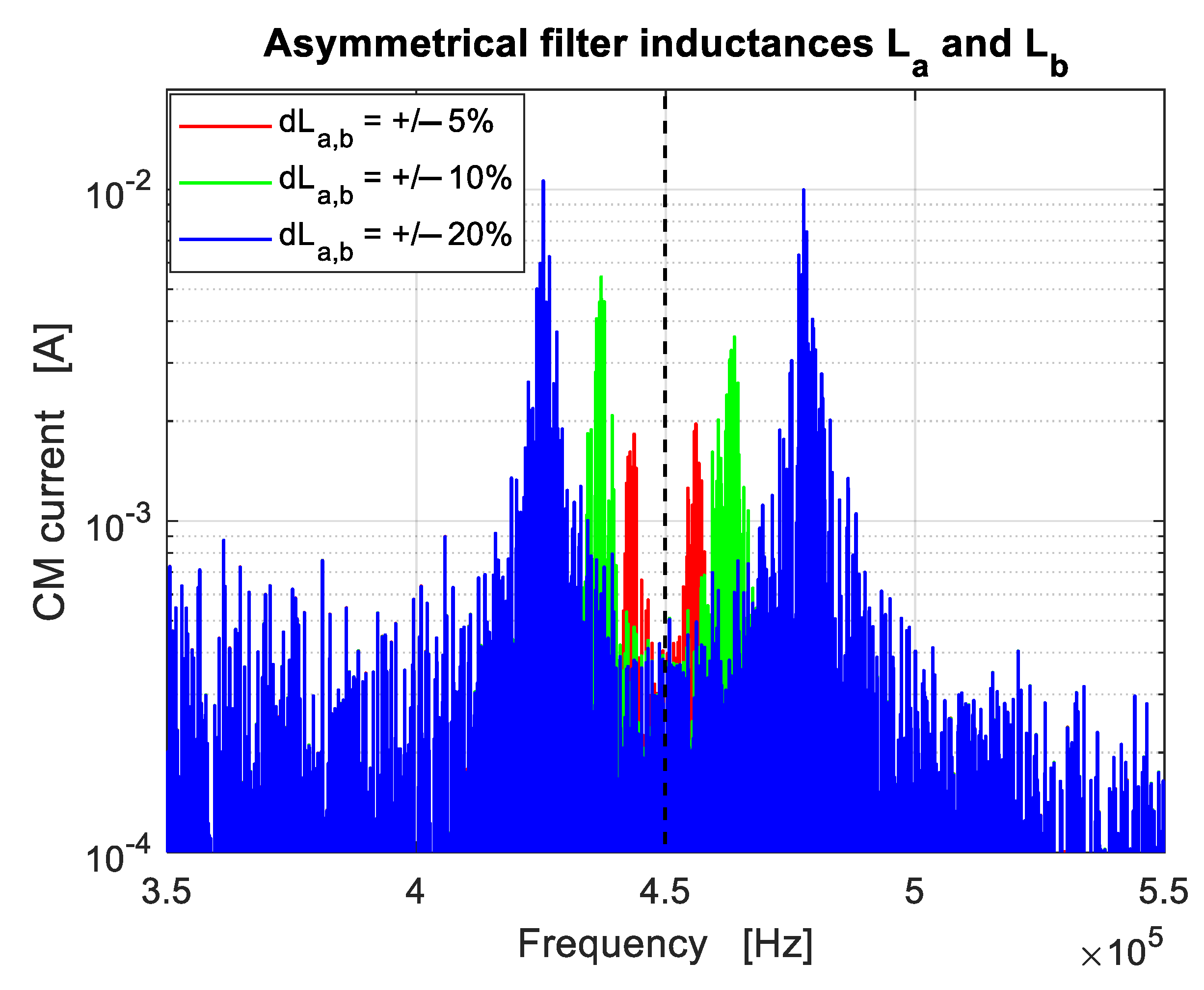
Figure 8 shows the case of simultaneous deviations of the inductances
and
. By selecting, as in the previous case,
, according to (25) and (26), the two eigenvalues are
, and the two resonance frequencies
. Thus, the two peaks have frequency separation
. Three different percent values were assumed for
(i.e.,
,
, and
). The corresponding frequency separation of each couple of peaks are 13, 26, and 52 kHz. This point is confirmed by
Figure 8. The same remark mentioned in the previous case holds for the location of peaks when
.
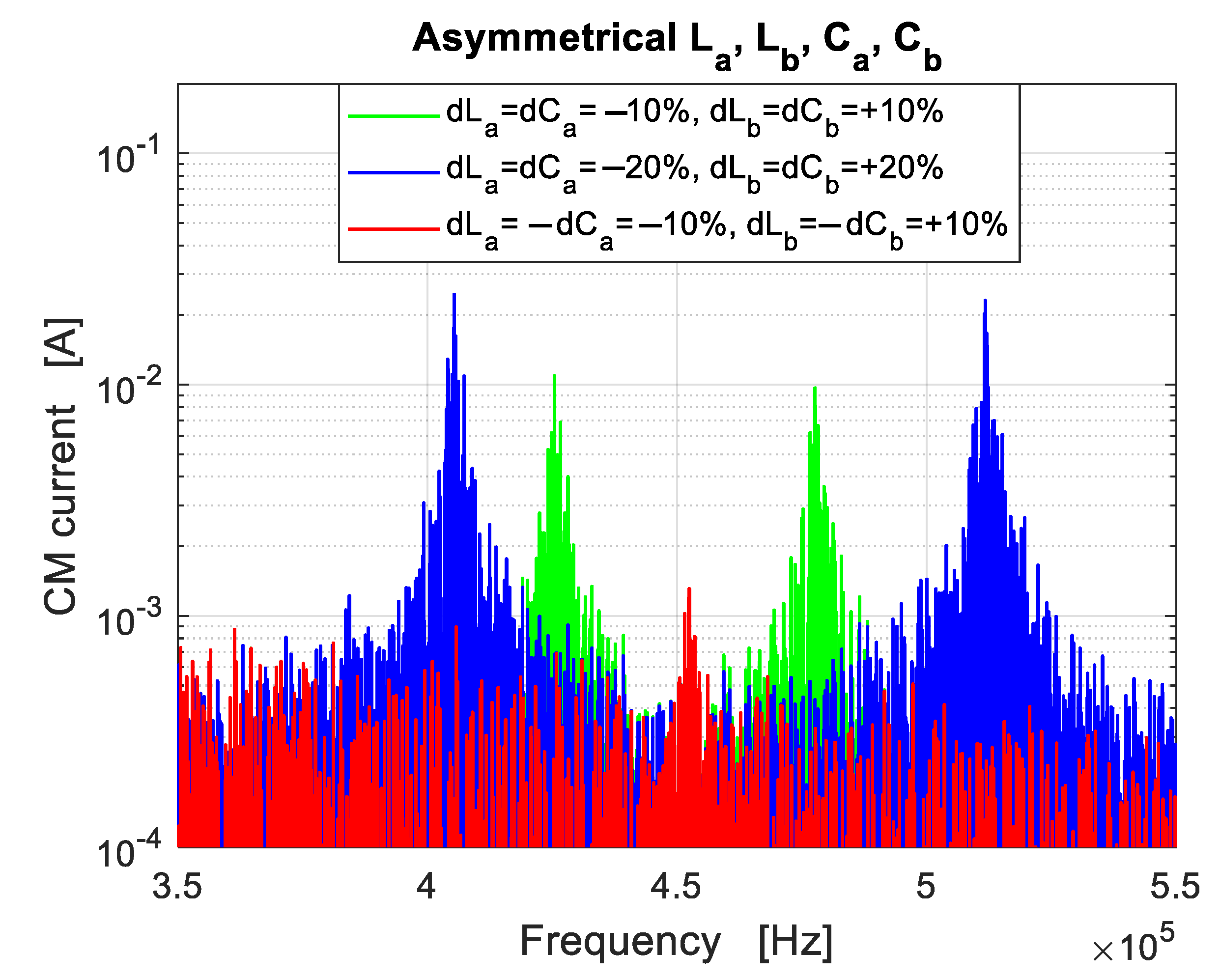
Figure 9 shows the impact of simultaneous deviations of both filter inductances and capacitances. Two cases can be put into evidence. First, the deviations of components
a (i.e.,
and
) have the same sign (i.e.,
), as well as the deviations of components
b (i.e.,
). In this case, the two peaks are reinforced by the two filter components. In the second case, the deviations of components
a have opposite sign (i.e.,
), as well as the deviations of components
b (i.e.,
). In this case, the action of the two filter components are in the opposite directions, resulting in a contrast to the frequency shift of the peaks. To highlight this phenomenon, a first simulation was performed with
and
(green curve). The effect of each deviation is doubled. In particular, the frequency separation between the two peaks is doubled with respect to
Figure 8. A second simulation (blue curve) was performed by doubling the relative deviations (and keeping the same signs as before). The frequency separation of the two peaks is doubled with respect to
Figure 8. Finally, a simulation with opposite sign was performed (red curve) (i.e.,
and
). Since the deviations of the two filter components act in opposite directions, the result is only one peak with small magnitude and negligible frequency shift.
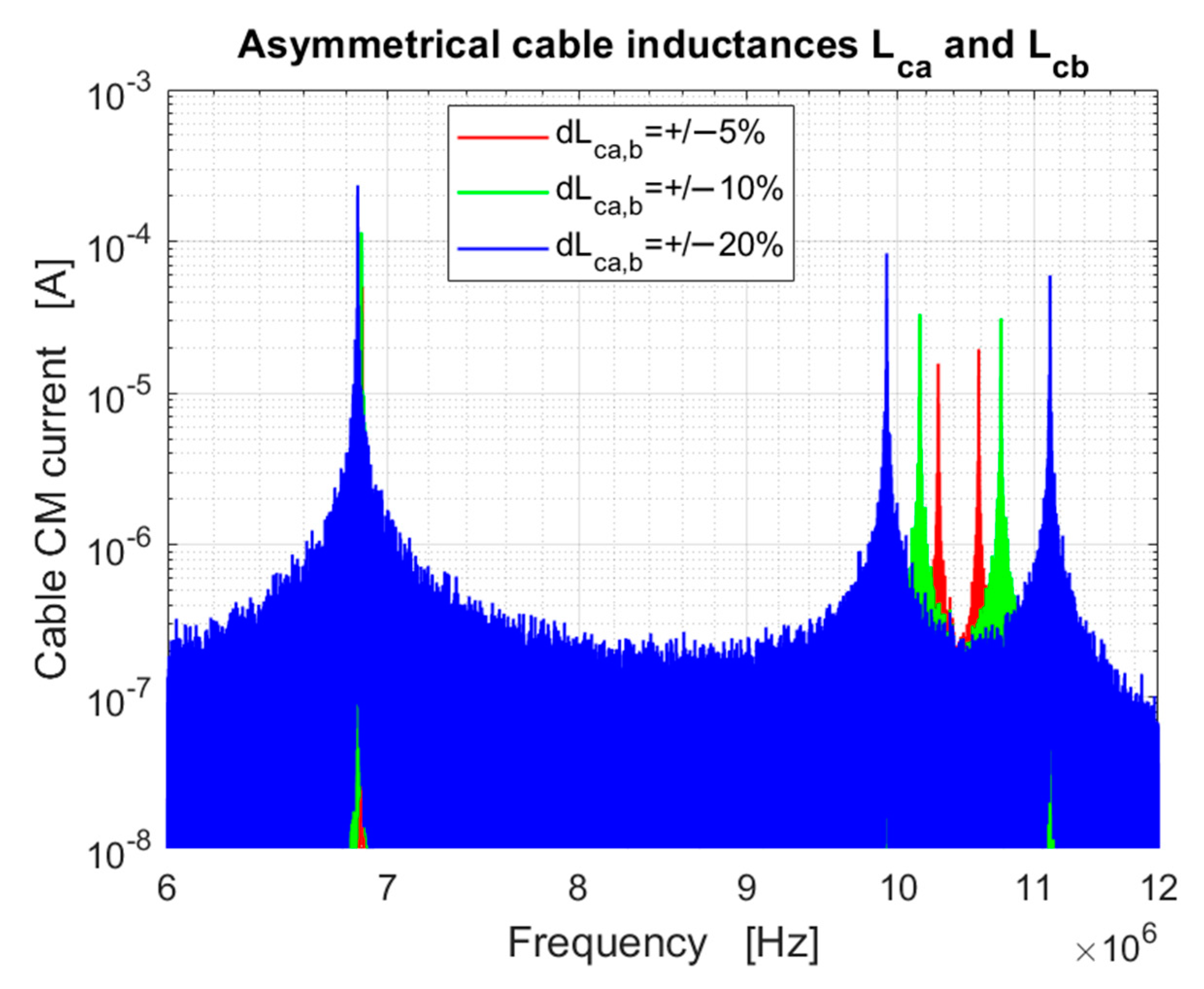
Figure 10 shows the amplitude spectrum of the cable CM current (see
in
Figure 3) for different deviations of the cable self-inductances. This set of simulations was performed to show how the DM circuit can inject current into the CM circuit at any system asymmetry (i.e., not only the LC filter). In case of cable asymmetry, the DM resonance involving the cable leads to current injection into the cable CM circuit. According to
Figure 4a, the cable is responsible of a DM resonance corresponding to its DM inductance
(i.e., the difference between the self and the mutual inductances) and the total capacitance consisting in the sum of the cable capacitance
and the parasitic capacitances
and
(in fact, at high frequencies the branch
can be ignored). Thus, the frequency of the DM resonance is given by
. The self-inductance deviations were selected such that
, and three different values were selected for
(i.e.,
,
, and
). According to
the corresponding frequency separation of each couple of peaks were 300 kHz, 600 kHz, and 1.2 MHz. This is confirmed by
Figure 10, where another spectral line can be clearly seen at 6.9 MHz. Such spectral line is independent of cable asymmetry since it is related to the resonance of the CM circuit (see
Figure 4b):
, where
.
5. Statistical Analysis
Analytical results derived in
Section 3 allow accurate evaluation of DM resonances injected into the CM circuit in case of known asymmetrical values of the filter components. When we are interested in the effects of component tolerance, however, a statistical approach is more suited to the objective. The statistical analysis of the eigenvalues (17) and (25), and the related resonance frequencies (21) and (26), will be derived in this Section by treating all the deviations
(i.e.,
and
) as random variables. Two cases will be investigated, corresponding to two different statistical distributions for the random variables
: Gaussian and Uniform distributions. In order to obtain unitary and normalized results, the following transformation of random variables will be investigated:
where
,
,
for capacitances, and
,
,
for inductances. The corresponding normalized resonance frequencies are given by:
5.1. Gaussian Distribution
Let us assume
as uncorrelated Gaussian random variables with zero mean and variance
. The transformation (29) requires first the analysis of the random variable:
By taking into account that
, for the mean value and the variance of
we obtain [
26]:
Therefore, the mean value and the variance of
can be approximated as:
where the approximations through the first and second order derivatives were used (i.e., the Taylor series approach) [
26,
27].
From (29) and (33) the mean values and the variance of
are given by:
Notice that since and are defined as the sum of uncorrelated random variables, their distribution can be approximated as a Gaussian distribution with mean values and variance given by (34).
Finally, the mean value and variance of the normalized resonance frequencies (30) can be approximated as:
The probability density function (PDF) of (30) can be obtained through the theorem of the transformation of random variables [
26]. By taking into account that, as mentioned before,
can be approximated by Gaussian random variables, the PDF of the two normalized resonance frequencies are given by:
where
and
are given by (34).
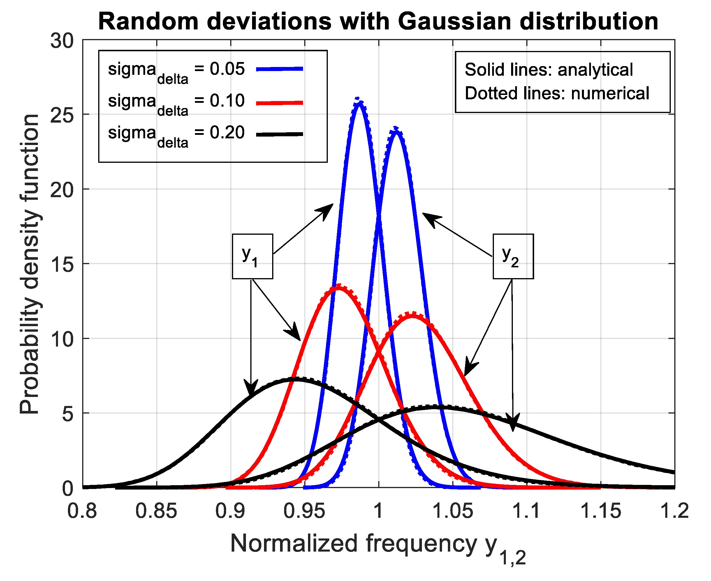
Figure 11 shows the behavior of the two PDFs (36) for three values of
(i.e., 0.05, 0.10, and 0.20). The analytical curves corresponding to (36) (solid curves) are compared with numerical results obtained by repeated run analysis (dotted curves). Notice that for each
the two PDFs show one peak on the left and one peak on the right side of the normalized frequency 1. By increasing
, the two peaks decrease in magnitude and move away from 1, whereas the PDF spread increases. For
the left resonance can decrease till about
, whereas the right resonance can increase till about
. For
0 the left resonance can decrease till about
, whereas the right resonance can increase till about
. For
the left resonance can decrease till about
, whereas the right resonance can increase till about
.
5.2. Uniform Distribution
Let us assume as uncorrelated Uniform random variables with zero mean and variance , where is the range of each random variable (i.e., the interval ).
By taking into account that
, for the mean value and the variance of
we obtain:
Therefore, the mean value and the variance of
can be approximated as:
where the approximations through the first and second order derivatives were used [
26,
27].
From (29) and (33) the mean values and the variance of
are given by:
Notice that since and are defined as the sum of uncorrelated random variables, their distribution can be approximated as a Gaussian distribution with mean values and variance given by (39). In this case, however, a worse approximation is obtained with respect to the Gaussian case because Uniform distributions have limited range.
Finally, the mean value and variance of the normalized resonance frequencies (30) can be approximated as:
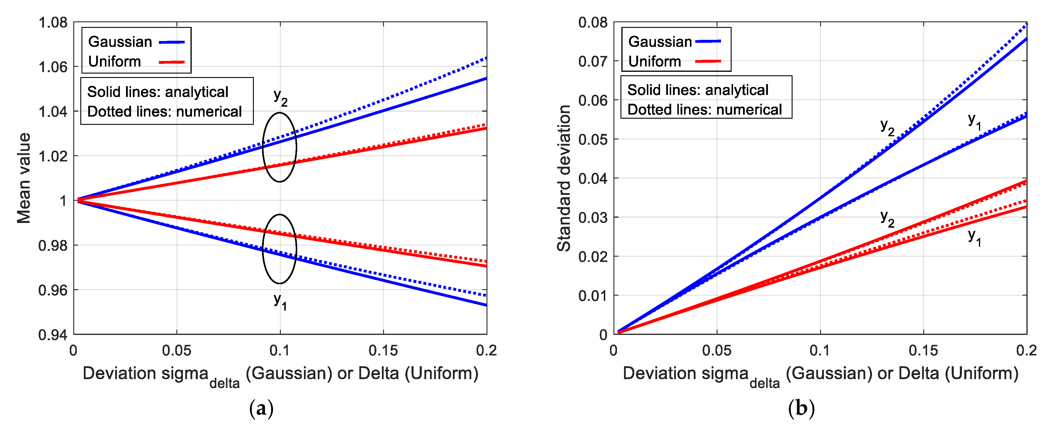
Figure 12a,b shows the behavior of the mean value and the standard deviation of
as functions of
(red lines). Analytical results (40) (solid lines) are compared with numerical results obtained through repeated runs (dashed lines). The same figure shows the behavior of the mean value and the standard deviation of
in the Gaussian case (35) (blue lines) for
in the same range of
. Gaussian distribution results clearly in larger spread of the resonance frequencies.
The PDF of (30) could be readily obtained through the theorem of the transformation of random variables as in the Gaussian case. By taking into account that can be approximated by Gaussian random variables, the PDF of the two normalized resonance frequencies are given by (36), where and are given by (40).


