When a constructive parameter of the modules of TCW-MPMSMs is subjected to tolerance analysis, more than a single module should be taken into account to obtain comprehensive conclusions. In a real manufacturing process, multiple modules can exhibit failures (and combinations of them) and therefore a deeper analysis is required. For a single parameter subjected to analysis, when n failures are considered in addition to the faultless condition, a total of possible combinations in a single module must be studied. This holds true for a discrete tolerance analysis. For instance, considering the lowest dimensional tolerance for the angular displacement, each module can be either centered (faultless), displaced 0.05° clockwise or displaced 0.05° counter-clockwise regarding its axis of symmetry, which sums up three combinations to be evaluated and two possible failures () for each stator segment.
Hence, to analyze a single dimensional tolerance (e.g., angular displacement of modules) regarding all modules of the selected 24-slot machine, the model must be evaluated roughly 4000 times in presence of one failure per module (n = 1) and 500,000 times in case of two failures per module (n = 2), which is infeasible by means of FE simulations only.
4.1. Superposition Method
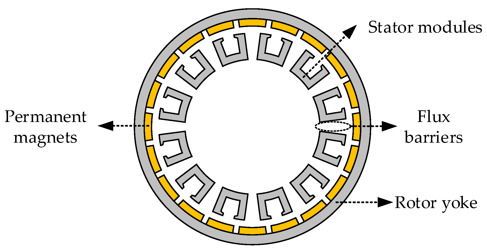
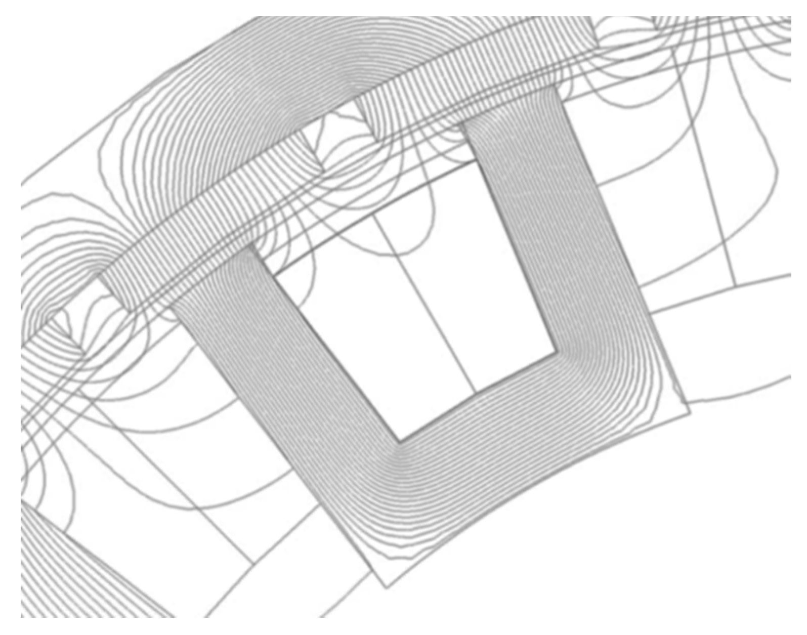
For TCW-MPMSMs with the number of slots given by (1), modules are ideally magnetically decoupled from each other, as depicted in
Figure 10, which shows the no-load flux lines of a 24-slot 28-pole machine.
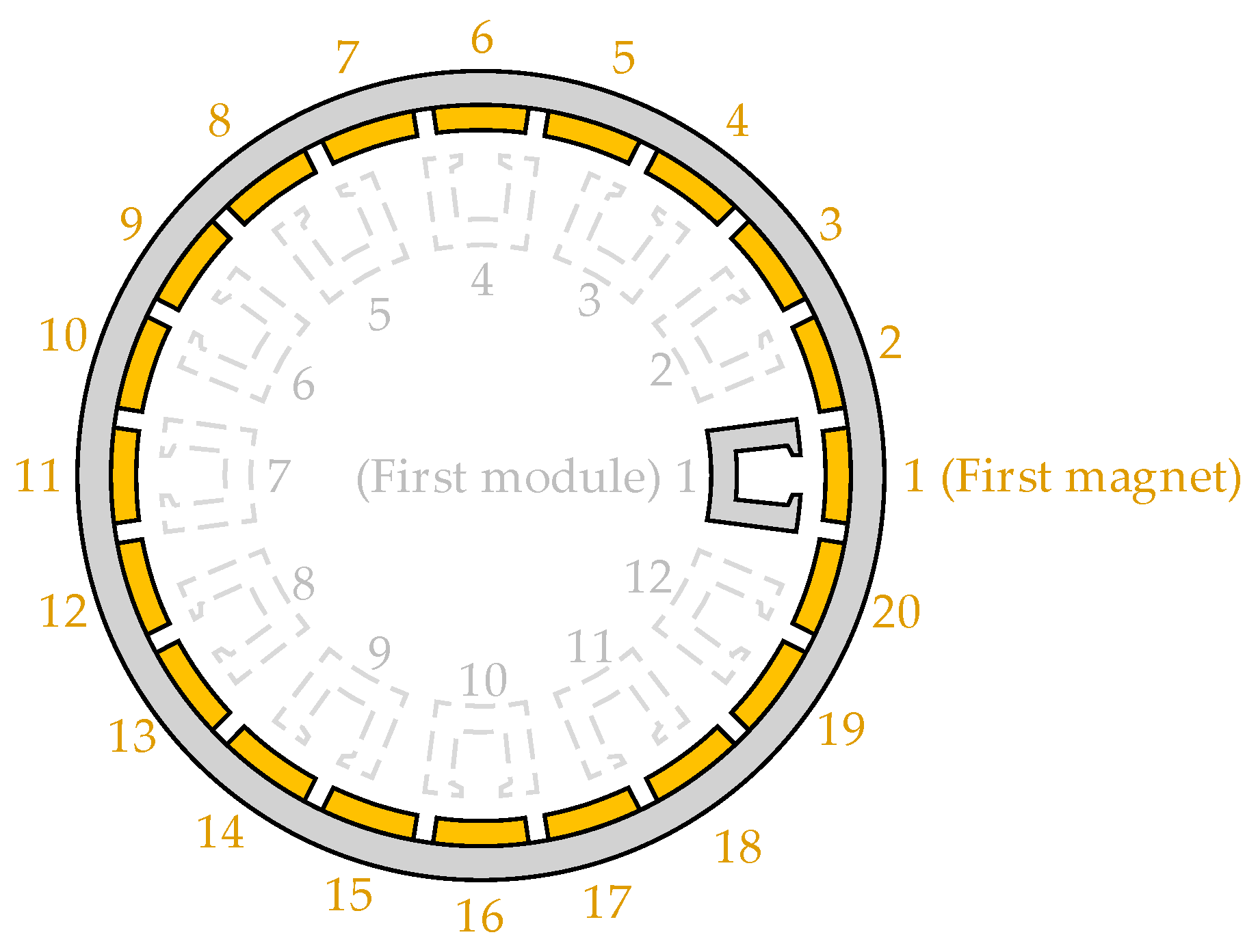
A negligible number of magnetic field lines link two or more modules, while most of the lines close the magnetic circuit through a single module. Hence, the overall cogging torque can be synthesized considering the contribution of each stator module separately. In such case, a FE simulation of the machine with only one active module should be carried out, as shown in
Figure 11. The contributions of the other modules can be obtained from the cogging torque of the active module and introduction of an appropriate offset angle.
Considering a reference frame in which the first magnet is aligned with the first stator segment, as shown in
Figure 11, the second magnet will be shifted by 360/(2
p) degrees with respect to the first one, and the second stator segment will be shifted by 360/(
Qs/2) with respect to the first module. Therefore, the second magnet will be misaligned with respect to the pertinent module by 360/(
Qs/2) − 360/(2
p). Following a similar analysis, the general expression for the angular displacement (in mechanical degrees) of the cogging torque produced by the
i-th module is given by
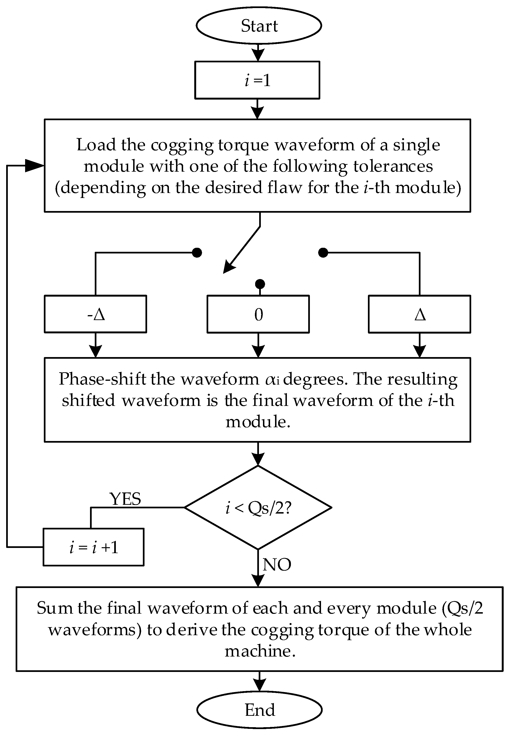
The overall cogging torque can be obtained by summing up the shifted waveforms of each module.
Different tolerances can be included in this superposition method. For instance, if angular displacement needs to be evaluated, the offset angle for the cogging torque waveform of each module is required to be adjusted, following the pertinent displacement tolerance. The general algorithm of the superposition method is described in the flowchart shown in
Figure 12, which allows semi-analytical estimation of the cogging torque waveform for faultless and faulty machines.
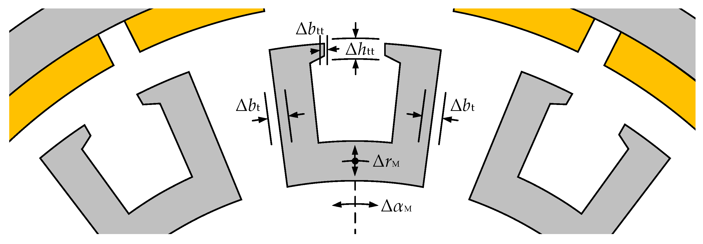
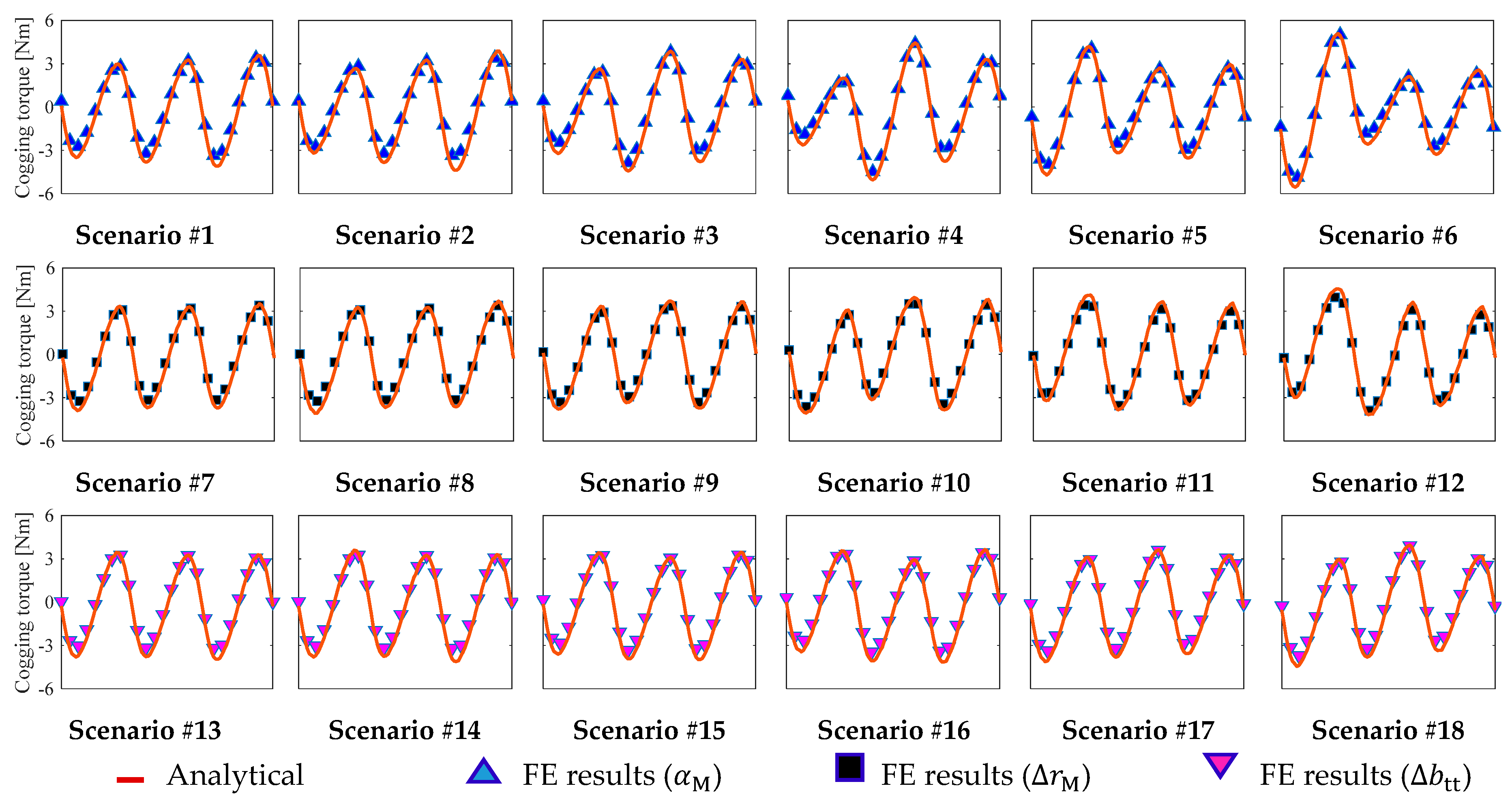
In order to validate the proposed superposition method, eighteen faulty scenarios are defined. These scenarios allow evaluating the cogging torque when angular displacements, radial displacements, and tooth–tip width deviations are applied to the modules separately. For example, the first six scenarios evaluate the angular displacement of the modules, while neglecting the other tolerances (radial displacement and tooth–tip width deviation), and the same principle is applied for every six scenarios. Also, the scenarios evaluate the presence of faults in one, three and seven modules of the machine following the same fault pattern.
Table 2 groups the main data of the validation scenarios, including the tolerance put through validation, the degree of tolerance and the modules affected by faults. The comparison of the cogging torque between FEA and the superposition method, for a 24-slot 28-pole machine is presented in
Figure 13, considering the aforementioned scenarios.
It can be observed that in all 18 cases, the results provided by the different methods show good correspondence, even though the changes are large from scenario to scenario, hence proving the accuracy of the proposed method.
4.2. Results and Robustness Analysis
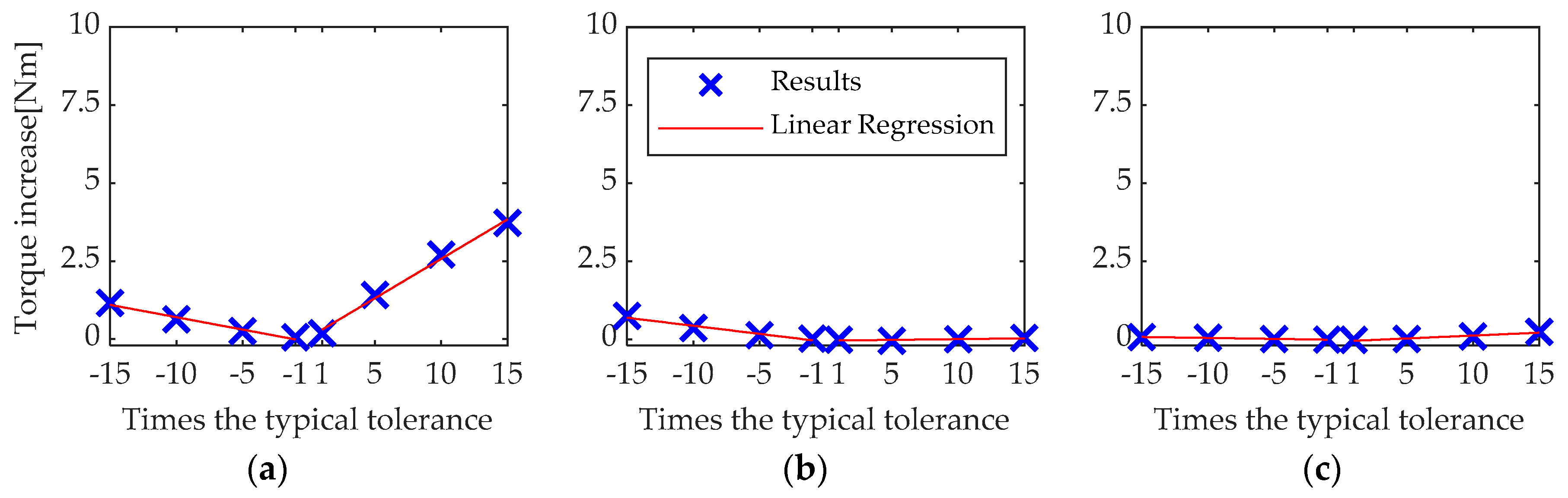
Aiming to evaluate the robustness of the selected topology, a full-range tolerance analysis considering two failures for each tolerance (
) is carried out by means of the superposition method presented in the previous subsection. The cases of study cover four different tooth–tip faultless/nominal widths (from 0 to 6 mm) and two magnet-to-pole arc faultless/nominal values from 0.8 to 0.9, summing up eight designs to be analyzed, as shown in
Table 3.
In
Section 3, angular and radial displacements of the modules, as well as the tooth–tip width tolerance, developed the most significant impacts on the cogging torque. Therefore, upon each of the eight designs, tolerance degrees of 0.05° and 0.10° will be considered for the angular displacement, and tolerance degrees of 0.1 and 0.2 mm will be applied both to the radial position and tooth–tip width of the modules.
A tolerance degree of Δ means that each module can have positive deviation (Δ), null deviation (0) or negative deviation (−Δ). E.g., a tooth–tip width subjected to a degree of tolerance of 0.1 mm means each one of the 12 modules of the machine (for a 24-slot 28-pole machine) can have tooth tips of width , or , where is the faultless tooth–tip width.
To improve the visualization of the large amount of data obtained from this methodology, a statistical overview of the results is presented. A probability density distribution of the normalized peak-to-peak value of the cogging torque (
) of each design, when all tolerance combinations are considered, is derived.
is given by
where
is the mean value of the full-load electromagnetic torques of the design, which depends, among other parameters, on the tooth–tip width and the magnet pole-arc ratio [
10].
, for a TCW-MPMSM, can be approximated by using the no-load flux density distribution in the airgap of the machine and the linear current density [
27], as:
where
is the stator outer diameter;
is the no-load flux density distribution in the airgap [
10],
is the linear current density along the perimeter of the stator, which depends on the number of turns, the winding factor and other parameters; and
is the effective core length.
Table 3 summarizes the mean value of the electromagnetic torque obtained with (6) for the eight designs analyzed.
After obtaining the probability density distribution of a design, two values are highlighted: the faultless/ideal case, and the expected value (probabilistic median of all tolerance cases).
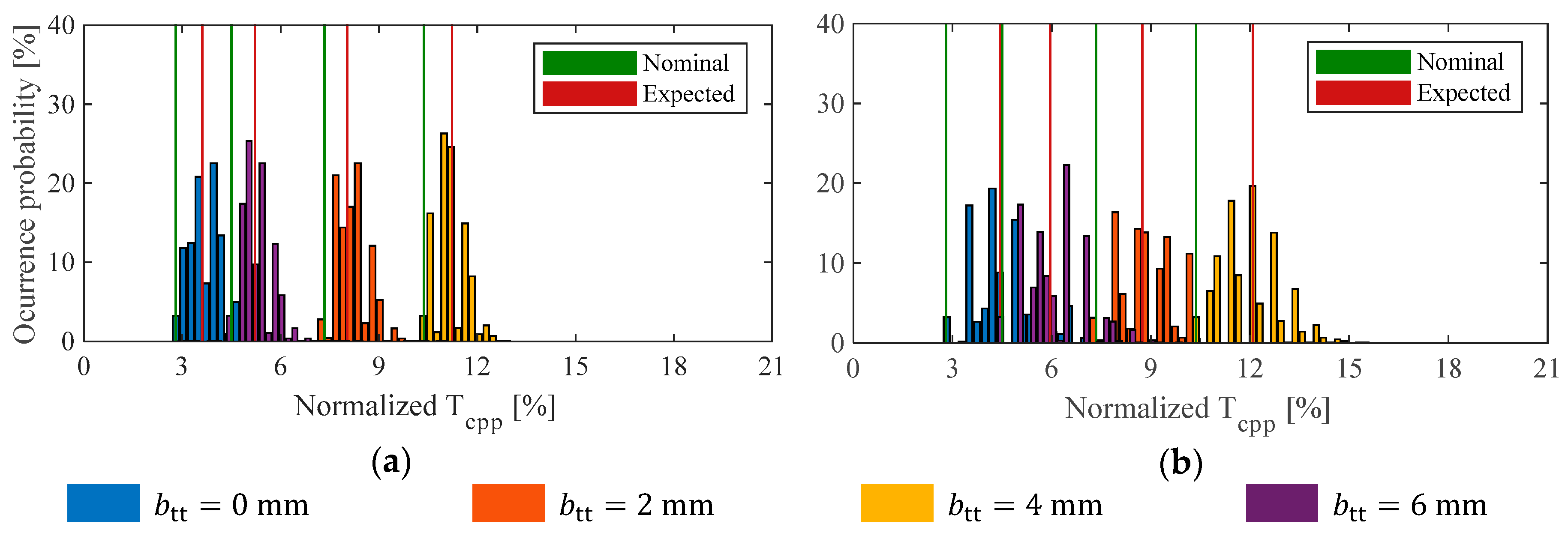
In
Figure 14, the probability distribution of
of the four designs with
(Design #1 to #4) are shown.
Figure 14a shows the distribution when a tolerance degree of 0.05° is considered for the angular displacement of modules, whilst
Figure 14b shows the distribution when the tolerance degree is 0.10°. Overall computation time for obtaining the results shown in
Figure 14 was approximately 3 h, considering five FE simulations of one-magnet machine, following the procedure explained in the previous subsection, and carrying out the post-processing by means of the proposed superposition method. As roughly 1 million combinations were evaluated, carrying out this analysis entirely through FEA would be impractical to perform, as each simulation lasts 30 min until completion on a 6-core 12-thread processor.
From
Figure 14, it can be noted that the
density distributions (shown as groups of colored bars) substantially change for different values of tooth–tip width
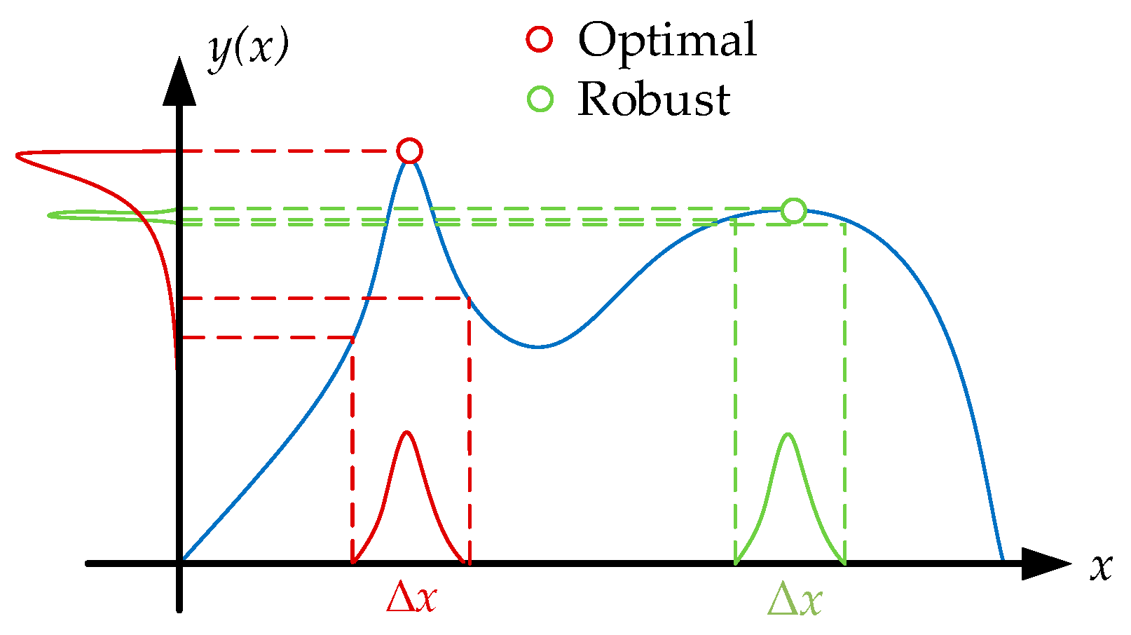
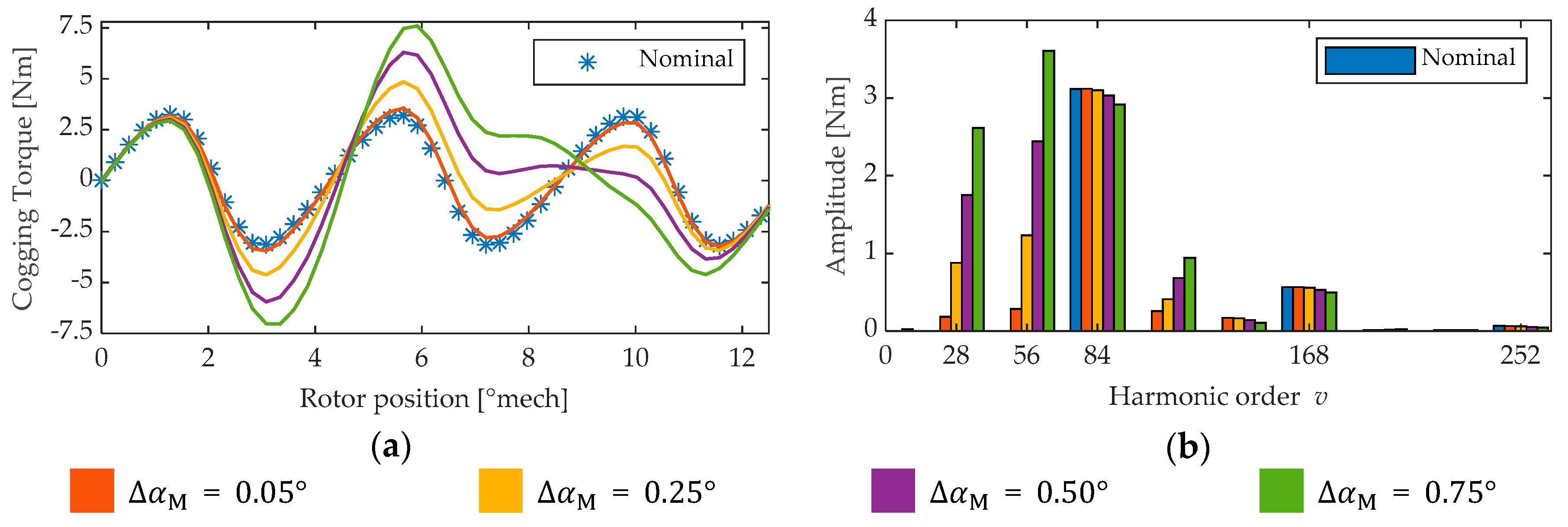
. More importantly, angular displacement of the modules causes
to be higher than the nominal value, in agreement with the behavior shown in
Figure 5.
The expected
value, which is the probabilistic median of the results obtained for all possible faulty combinations, is also higher than the nominal one for the four designs. When the tolerance degree doubles, as depicted in
Figure 14b when compared with
Figure 14a, similar conclusions can be drawn: the expected cogging torque is higher than the nominal/faultless for all cases with
. As the tolerance degree increases (from 0.05° to 0.10°), the difference between the expected and the nominal values also increases.
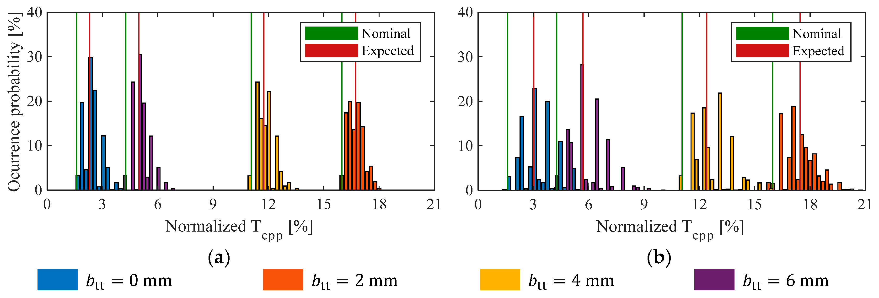
On the other hand,
Figure 15 shows the probability distribution of
of the four designs with
(Designs #5 to #8), evaluating two degrees of tolerances: 0.05° for the angular displacement of the modules in
Figure 15a, and 0.10° in
Figure 15b. From both figures it can be noted that, unlike the previous designs with
, adopting 2 mm wide tooth–tips develops the worst nominal cogging torque among all designs with
. Notice that the expected
value (highlighted as a vertical red line) is higher than the nominal one (highlighted as a vertical green line) for the four designs, irrespective of the selected degree of tolerance.
With the aim of quantifying this behavior and describing the robustness of the eight designs, a robustness error (
) is defined as
Table 4 summarizes the main results of the evaluation of the eight designs, when a tolerance degree of 0.05° is applied to the module angular position. These results take into account the nominal and expected values of
, the difference between nominal and expected (
), and the robustness error (
).
Table 5 groups the results when a tolerance degree of 0.10° is evaluated.
From both tables, it can be noted that
is always positive, and its value is similar for the eight designs when a certain degree of tolerance is considered. This means that
can be considered as independent of the tooth–tip width as well as being independent of changes to the arc-to-pole ratio changes (e.g., in
Table 4 for all eight cases).
When the degree of tolerance doubles (from
Table 4 to
Table 5),
approximately doubles. This can be seen from Design #1 (Δ
= 0.8 and
= 0 mm) results:
is 0.8% in
Table 4 (a tolerance degree of 0.05°), whereas
is 1.6% in
Table 5 (a tolerance degree of 0.10°). Therefore, it can be stated that
mainly depends on the considered tolerance degree, while the nominal tooth–tip width and the pole-to-arc ratio show negligible influence. Furthermore, even when there are large differences between the nominal cogging torque of the designs, i.e., when different tooth–tips and pole-to-arc ratios are adopted, the variation of the cogging
due to mechanical tolerances is relatively constant for all the designs, when the same tolerance degree is considered.
On the other hand, in
Table 6, the main results of the evaluation of the eight designs, for a tolerance degree of 0.1 mm over the radial displacement, are summarized, while
Table 7 groups those results for a tolerance degree of 0.2 mm over the radial displacement.
Table 8, in turn, groups relevant results of the evaluation of the eight designs, when a tolerance degree of 0.1 mm over the tooth–tip width is considered, are summarized.
Table 9 presents the results when a tolerance degree of 0.2 mm is evaluated.
Similar conclusions can be obtained from these four tables (
Table 6,
Table 7,
Table 8 and
Table 9) when compared to
Table 4 and
Table 5: the impact of radial displacement and tooth–tip width tolerances on the cogging torque of the machine is approximately independent of the nominal tooth–tip width and pole-to-arc ratio, and the difference between the expected and the nominal
mainly depends on the degree of tolerance evaluated.
However, it can be noted that tooth–tip width tolerances are not as relevant as angular displacement or radial displacement of the stator segments on modular machines. This can be seen, for example, by analyzing Design #8: angular displacement tolerances cause a robustness error of 16% and radial tolerances cause an error of 14%, whereas tooth–tip width tolerances generate a 5% error.
These findings further determine the value of the robustness error of each design: In (7), the numerator () of the expression has been found to be relatively constant for a certain tolerance degree. Then, can be taken as inversely proportional to the nominal cogging torque peak-to-peak value. This can be explained by separating the cogging torque “sources”. One “source” is the geometry of the design and the slot–pole count: the faultless machine generating the rated cogging torque, and the asymmetries/tolerances are another “source”, generating . Therefore, minimizing the first source, i.e., the nominal cogging torque, will then lead to a higher relative cogging increment due to tolerances and a higher robustness error.
From the analysis, it can be concluded that, for lower cogging torque requirements, it will be necessary to have tighter tolerances, as lower nominal cogging torque designs exhibit lower robustness. This can be seen by analyzing the results of Design #5, which has the lowest nominal cogging–torque peak-to-peak value among the eight selected designs. However, for this design is 88% (the highest among all the designs), which means that the expected , once typical mechanical tolerances are considered, will be 88% higher (almost twice) than the original value. The optimization process of a machine, in its dimensioning stage, must be carried out carefully to integrate these properties if the goal is low cogging torque.

 ,
, 


