A Multi-Objective Evolutionary Algorithm Based on KNN-Graph for Traffic Network Attack

Abstract

The research of vulnerability in complex network plays a key role in many real-world applications. However, most of existing work focuses on some static topological indexes of vulnerability and ignores the network functions. This paper addresses the network attack problems by considering both the topological and the functional indexes. Firstly, a network attack problem is converted into a multi-objective optimization network vulnerability problem (MONVP). Secondly to deal with MONVPs, a multi-objective evolutionary algorithm is proposed. In the new approach, a k-nearest-neighbor graph method is used to extract the structure of the Pareto set. With the obtained structure, similar parent solutions are chosen to generate offspring solutions. The statistical experiments on some benchmark problems demonstrate that the new approach shows higher search efficiency than some compared algorithms. Furthermore, the experiments on a subway system also suggests that the multi-objective optimization model can help to achieve better attach plans than the model that only considers a single index.

1. Introduction

The complex network is a popular formal description of complex systems. Some typical complex networks include social networks [1,2], internet of things [3,4], transportation networks [5], Internet networks, power system networks [6] and so on. Based on the complex network model, scholars can perform a variety of analyses, such as the shortest path [7], community detection [8] and so on. In real-world applications, what we most concern might be the complete function of the complex system. In other words, if a complex system cannot complete its mission, it might be broken. However, in most cases, systems losing part of its function rather than all may still work in a sense. So how to describe the network quantitatively becomes a challenge task. A large number of research results indicate that a complex network will suffer performance degradation due to various modes of attacks [5,9,10]. Attacks may come from many sources, such as a disconnection of the Internet line, a damage to the transportation network road, and a firepower of the military network.

The vulnerability is widely used to analyze complex networks. It can be simply understood as the degree to which a network maintains its original function when it is attacked. The purpose of network vulnerability research is to find the weak and vulnerable nodes of a network [11]. Network vulnerability analysis plays a key role in many real-world applications. For example, the vulnerability analysis of hydro-power resource allocation network can provide effective suggestions for resource allocation. For a network of confrontation type, such as military combat system networks, the vulnerability is important to analyze and find the best attack strategy in the operation. The vulnerability analysis of the logistics transportation network helps find the key nodes in the transportation channel. Whether for attacking nodes to damage the network, or optimizing the network structure before the attack, or repairing the network after the attack to restore the function as much as possible, vulnerability analysis can provide highly targeted for these problem instructions.

The index design and/or numerical analysis of network vulnerability have attracted much attention. Basically, the vulnerability analysis depends on the type of a network. To analyze the vulnerability of the power system network, Biswas et al. [12] used graph theory knowledge to analyze whether a contingency will create a saturated cut-set in a meshed power network. For computer networks, Yan et al. [13] used attack graph theory to analyze the network estimation vulnerability of the optimal compensation set. For the military combat network, Liu et al. [11] used the analytic hierarchy process to give the military combat network nodes various attributes such as firepower, control, and intelligence. For the transportation network, Liu [14] et al. conducted a quantitative analysis on the topological characteristics of China Comprehensive Transportation Corridors and Hubs (CCTCH) based on graph theory and complex network theory. Their research incorporates topological and non-topological factors such as node degree, betweenness, socioeconomic factors (i.e., GDP, population, GDP per capita).

In the previous work, the vulnerability is often regarded as a static topological logic index. However, in many cases, people are more concerned about how much the network’s functions decline when facing specific attacks. In other words, the network’s vulnerability should be oriented to specific attacks and specific functions. For example, a same transportation route should show different vulnerabilities when carrying people and goods, subjecting to random natural disasters and man-made terrorist attacks. Therefore, the vulnerability of a network should be related to specific situations.

Regarding the network vulnerability as a confrontation between the attacker and the network itself, then for the attacker, the most concerned issue is to achieve the maximum attack effect with the least possible attack cost. The attack cost can be seen as how many nodes, links, or network equipment have suffered losses. The attack effect can be measured as the degree to maintain the original functions after being attacked. To consider the two indexes simultaneously, we could model the vulnerability as a continuous multi-objective optimization problem (MOP).

With regard to continuous MOPs, since Schaffer [15] first applied an evolutionary algorithm to solve MOPs, multi-objective evolutionary algorithms (MOEAs) has been the most popular approach for dealing with MOPs [16], which can achieve an approximate solution set of the PS in one run. According to the basic ideals adopted by MOEAs, which have developed in the past few decades. MOEAs can be roughly divided into the following three categories [17]:

(1)

Pareto dominance based MOEAs, such as the nondominated sorting genetic algorithm II (NSGA-II) [18] and improved strength Pareto evolutionary algorithm (SPEA2) [19];

(2)

Performance indicator based MOEAs, such as the indicator-based evolutionary algorithm (IBEA) [20] and S-metric selection evolutionary multi-objective optimization algorithm (SMS-EMOA) [21];

(3)

Decomposition based MOEAs (MOEA/D), MOEA/D [22] is different from the above two kinds of algorithms, since it is not a specific algorithm, but a general algorithm framework that can be incorporated into evolutionary strategies [23,24].

However, those aforementioned evolutionary multi-objective optimization (EMO) approaches focus on environment selection methods. In fact, offspring reproduction also has a remarkable influence on MOEAs. What is more, it should be worth our attention that the structure of Pareto Solution Set (PS) emerges as a regularity property, that is the PS of a bi-objective optimization problem defines a piece-wise continuous curve, meanwhile the PS of a tri-objective optimization problem defines a piece-wise continuous surface. An efficient EMO method should make use of thus problem knowledge to guide its search directions. With this consideration, the clustering learning-based mating restriction strategies are popular practices [25,26,27]. In our previous work, the adaptive population structure learning and multi-source mating restriction [28,29] both have well performance while solving complex MOPs, however the clustering operation also brings a lot of computing overhead. Hence, in this work, we aim to find other low computational cost approach to learn the PS manifold structure for mating restriction in MOEA reproduction.

Considering these limitations, we aim to study the vulnerability of the network by constructing a new model and evolutionary algorithm framework. This paper attempts to construct the nearest neighbor relationship of parent solutions, and proposes to use a K-nearest-neighbor Graph (KNN-Graph) that can effectively express the absolute position distribution relationship of complex high-dimensional data. By using the KNN-Graph based reproduction operator, we design a new framework of MOEA. To assess this framework, this paper collects part of the Shanghai Subway network and its daily passenger flow data to construct a traffic network for vulnerability analysis. The main contributions of the paper are summarized as follows.

(1)

We design a new vulnerability index based on the traffic information that represents the network function. This makes the result more suitable for specific functions of a traffic network.

(2)

We regard the vulnerability of the network as a confrontation between the network attacker and the network itself and convert it into a multi-objective optimization problem by considering the attack cost and attack efficiency simultaneously.

(3)

We propose a KNN-Graph based reproduction operator for MOEAs to improve the convergence of MOEAs.

The remainder of this article is organized as follows: Section 2 introduces a multi-objective optimization model for a traffic network attack and its evaluation indexes. In Section 3, we propose a new KNN-Graph based reproduction operator and design a new MOEA. In Section 4, we compare the new algorithm with some state-of-the-art MOEAs on some benchmark problems. We also apply the algorithm to the Shanghai subway network to assess its performance on real-world problems. In Section 5, we conclude the paper with some discussions for the future work.

2. Model of Network Attack

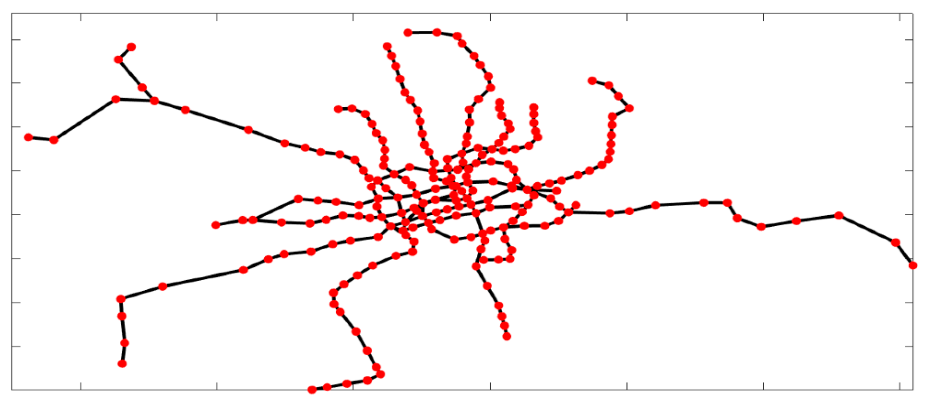
2.1. Subway Network Model

The Shanghai Subway was originally built in 1990. After the completion of 19 lines in 2021, the total length will reach 830 km. This paper selects 11 lines, Lines 1 to 11, from the Shanghai Subway system, with 232 stations and 256 edges. Among them, 16 stations have one neighbor station, 188 stations have two neighbor stations, five stations have three neighbor stations, 22 stations have four neighbor stations, and two stations can reach five stations directly. The four lines, Lines 1, 3, 7 and 8 connect the north and south areas and pass through the city center. Lines 2, 10 and 11 traverse east-west. Line 4 is a loop line, passing through downtown areas such as Xuhui District, Yangpu District, and Putuo District.

After collecting the geographic locations and daily passenger flow data of the Shanghai Subway website, this paper models the subway, and the result is showed in Figure 1.

2.2. Optimization Model Construction of Complex Network

For a given traffic network $\mathit{G}\left(\mathit{V},\mathit{E}\right)$, after suffering some kinds of attack, some links $e\in \mathit{E}$ and nodes $v\in \mathit{V}$ will be destroyed, and some nodes will become unconnectable with others. We defined the network after attacked as ${\mathit{G}}^{\prime }\left({\mathit{V}}^{\prime },{\mathit{E}}^{\prime }\right)$. And we also defined its nodes $v^{\prime }\in {\mathit{V}}^{\prime }$ and $e^{\prime }\in {\mathit{E}}^{\prime }$. All pairs of nodes in common networks have shortest path properties. This paper uses $dist\left(v_i,v_j\right)$ to represent the length of the shortest path from node $v_i$ to node $v_j$. The traffic network has the properties of ordinary networks, but also has its own unique properties. For a traffic network, each node has traffic that needs to be transmitted to other nodes. For example, the passenger flow that needs to be transmitted from one airport to another in the national air transport network. This paper uses $K\left(v_i,v_j\right)$ to represent the flow from node $v_i$ to node $v_j$.

As mentioned in Section 1, the vulnerability of a network can be designed as a simulation of an attack on the network, of which the two important issues are the attacker’s effect and cost. To address the two issues, we convert the problem about network vulnerability into the multi-objective optimization network vulnerability problem (MONVP), which is defined as follows.

$$min\left(f_1\left(\mathit{x}\right),f_2\left(\mathit{x}\right)\right),\mathrm{s}.\mathrm{t}.\mathit{x}\in \mathit{X}$$

(1)

where $\mathit{x}\in \mathit{X}$ is an attack plan for a given traffic network $G\left(V,E\right)$, $\mathit{X}$ denotes the set of all possible attack plans,$f_1\left(\mathit{x}\right)$ and $f_2\left(\mathit{x}\right)$ represent the efficiency and cost of an attack $\mathit{x}$. It should be noted that for the simplicity, we require that $f_1\left(\mathit{x}\right)$ and $f_2\left(\mathit{x}\right)$ are to be minimized. The details of the two objectives and the attack plan are introduced in detail in the following sections.

2.2.1. Network Transmission Efficiency $f_1\left(\mathit{x}\right)$

Existing researches often use the maximum connectivity component of the network [30] or network efficiency [31] to measure the vulnerability of the entire network. These methods can only reflect the nature of the network in logical topology but ignore the characteristics of the node itself. Each station in the subway network will have different characteristics due to the different geographical location, economic conditions, and population density. These differences will be concentrated in passenger traffic. So how to take passenger traffic into consideration is the focus of the definition of vulnerability index.

For a network $\mathit{G}\left(\mathit{V},\mathit{E}\right)$, it has many topological properties, such as the betweenness of nodes

$$Bet\left(v_i\right)={\displaystyle \sum }_{j\ne k\ne i}\frac{Path\left(v_i,v_j,v_k\right)}{Path\left(v_i,v_j\right)}$$

(2)

where $Path\left(v_i,v_j\right)$ is the number of the shortest paths from node $v_j$ to node $v_k$, $Path\left(v_i,v_j,v_k\right)$ is the number of paths from node $v_i$ to node $v_j$ through node $v_k$.

Links also have betweenness

$$Bet\left(e_{ij}\right)={\displaystyle \sum }_{l\ne m,\left(l,m\right)\ne \left(i,j\right)}\frac{Path\left(v_l,v_m,e_{ij}\right)}{Path\left(v_l,v_m\right)}$$

(3)

where $e_{ij}$ is the edge connecting node $v_i$ and node $v_j$. $Path\left(v_l,v_m\right)$ is the number of the shortest paths from node $v_l$ to node $v_m$, and $Path\left(v_l,v_m,e_{ij}\right)$ is the number of paths from node $v_l$ to node $v_m$ through edge $e_{ij}$.

Betweenness reflects the contribution of a node to network connectivity. In some cases, people are more concerned about whether a network is connected and can transmit traffic. In this paper, we call this network a traffic network. Obviously, this kind of network is more suitable for expressing its vulnerability with an index like betweenness.

This paper proposes the concept of network transportation efficiency. This index is based on the betweenness and is used to evaluate the functional decline of the traffic network. Given a traffic network $\mathit{G}\left(\mathit{V},\mathit{E}\right)$ and the remaining network ${\mathit{G}}^{\prime }\left({\mathit{V}}^{\prime },{\mathit{E}}^{\prime }\right)$ after suffering some kinds of attack, we define $T$ as the level of decline in network transportation efficiency.

$$\begin{gathered} T=\left({\displaystyle \sum }_{dist\left(v_i{}^{\prime },v_j{}^{\prime }\right)=\infty }K\left(v_i,v_j\right)+\left(\frac{T_a}{T_0}-1\right)\times {\displaystyle \sum }_{dist\left(v_i{}^{\prime },v_j{}^{\prime }\right)\ne \infty }K\left(v_i,v_j\right)\right) \\ /{{\displaystyle \sum }}^{}K\left(v_i,v_j\right) \end{gathered}$$

(4)

$$T_0={\displaystyle \sum }_{dist\left(v_i{}^{\prime },v_j{}^{\prime }\right)\ne \infty }\left(dist\left(v_i,v_j\right)\times K\left(v_i,v_j\right)\right)$$

(5)

$$T_a={\displaystyle \sum }_{dist\left(v_i{}^{\prime },v_j{}^{\prime }\right)\ne \infty }\left(dist\left(v_i{}^{\prime },v_j{}^{\prime }\right)\times K\left(v_i,v_j\right)\right)$$

(6)

while $K\left(v_i,v_j\right)$ is the passenger flow from node $v_i$ to node $v_j$ in the network $G$.$dist\left(v_i,v_j\right)$ is the shortest path distance from node $v_i$ to node $v_j$. $dist\left(v_i,v_j\right)=\infty$ means node $v_i$ is unconnected with $v_j$. In this paper, it is obviously that $dist\left(v_i{}^{\prime },v_j{}^{\prime }\right)\ge dist\left(v_i,v_j\right)\ne \infty$.

The greater the T, the greater the degree of network damage. In Equation (1) we hope to minimize $f_1\left(\mathit{x}\right)$, so we define the objective as

$$f_1\left(x\right)=-\mathit{T}$$

(7)

2.2.2. Network Attack Cost $f_2\left(\mathit{x}\right)$

According to the definition of ${\mathit{G}}^{\prime }$, this paper regards the attack behavior as the behavior that produces $V^{\prime }$ and $E^{\prime }$. According to the literature, attacks on the network can be divided into point attacks [9] and surface attacks [10]. Point attack selects some nodes or links to attack, while surface attack selects a certain area to attack and all nodes and links in this area will be damaged. Figure 2a shows the central area of Figure 1 and Figure 2b shows three surface attacks on the network. With the circular area as the surface, all lines and stations in the area are damaged. Although some stations are not attacked, the stations connected to them are destroyed. This makes them isolated stations, which can also be seen as damaged. The destroyed subway stations are shown in red. Point attack simulates random factors such as equipment failures and will not affect other stations. Surface attack often occurs because of deliberate attacks such as battlefield artillery strikes and urban terrorist attacks. This paper focuses on the surface attack.

The cost of a surface attack is related to many factors, and the most intuitive one is the radius of the attack area. As we just said, surface attack often occurs because of terrorist attacks or fire attacks. It’s easy to imagine that the larger the radius of the attack plan, the higher of cost. In other words, the cost is related to the ammunition equivalent. According to the equivalent physical formula, the equivalent of ammunition is proportional to the cube of the explosion radius:

$$f_2\left(\mathit{x}\right)={\displaystyle \sum }_{i=1}^{t}r{a}_i{}^3$$

(8)

while $f_2\left(\mathit{x}\right)$ is the attack cost, $t$ is the number of attacked areas, and $ra$ is the radius of an attacked area.

2.2.3. Representation of an Attack Plan $\mathit{x}$

In this paper, our target is to find an optimal attack plan. Therefore, we need to define a parameterized plan, i.e., a coding strategy to represent an attack plan that can be processed by an MOEA. The most commonly used way to encode a graph data structure is vector expansion of the adjacency matrix [32]. However, this may lead a long solution. According to the attack scheme introduced in Section 2.2.2 we encode the attack plan as follows in this paper:

$$\mathit{x}=\left[x_1,x_2,x_3;x_4,x_5,x_6;\dots x_{3t-2},x_{3t-1},x_{3t}\right]$$

(9)

while $x_{3i-1},x_{3i-2}$ are the coordinates of the center of the attack point, which is expressed in latitude and longitude, and $x_{3i}$ is the attack radius. This vector indicates there are $t$ attack points.

Figure 3 shows an example. The coded vector is [121.45, 31.22, 0.0471; 121.54, 31.01, 0.0032; 121.38, 31.11, 0.0102]. It represents three attacks near the Shanghai Subway. Their latitude and longitude are (121.45° E, 31.22° N), (121.54° E, 31.01° N) and (121.38° E, 31.11° N). Their radiuses are 0.0471, 0.0032 and 0.0102, respectively. This paper uses one latitude as the unit of distance, which is approximately 111 km. In other words, 0.0471, 0.0032 and 0.0102 in the code represent approximately 5.22 km, 3.55 km and 1.13 km.

After encoding the attack method, for each solution we can obtain an attack plan like Figure 2b.

3. An MOEA Based on KNN-Graph

3.1. Clustering Based Reproduction Operators

An MOEA maintains a set of candidate solutions, called population. It evolves the population by using the reproduction operator and the selection operator alternatively. The population will gradually approach the Pareto optimal solutions. It is clear that in the reproduction operation, choosing similar solutions for reproduction can improve algorithm convergence while selecting different individuals for reproduction can improve algorithm diversity. The clustering techniques can help to balance the algorithm convergence and diversity.

Li et al. [27] used the K-means algorithm to design a clustering-based self-adaptive mating restriction strategy, which can adaptively adapt different mating strategies for individuals in different clusters. Zhang et al. [33] designed a multi-objective evolutionary algorithm that can adaptively determine the probability of mating restriction, which is based on the nearest neighbor propagation and reproduction utility. It balances local exploration and global mining in the iterative process of the multi-objective evolutionary algorithm. After that, considering the expensive computational cost of clustering during evolution, Zhang et al. proposed a multi-objective evolutionary algorithm that organically combines clustering operations with evolutionary iterations [25], which allows the algorithm to evolve in one evolutionary process. The clustering operation is completed naturally. Considering the non-stationary nature of multi-objective evolutionary algorithm data, Sun et al. [26] designed an environment selection operator for online clustering of non-stationary and dependent data learning. Considering the non-stationary nature of multi-objective evolutionary algorithm data, Sun et al. [26] designed an environment selection operator for online clustering of non-stationary data learning. Its operator combines the iterative process of online agglomeration clustering with the evolution process of evolutionary algorithms. This allows the algorithm to complete the category update operations of adding individuals and deleting inferior solutions while selecting the environment. In addition, there are some multi-objective reproduction operators constructed from other perspectives [34,35,36].

Based on these studies, this paper proposes a reproduction operator based on KNN-Graphs to improve the search efficiency of MOEAs.

3.2. Establishment of KNN-Graph

To facilitate the description of the nearest neighbor graph, we first give the definition of the K-nearest-neighbor Graph.

Given a collection of data objects $\mathit{P}\mathit{o}\mathit{p}\mathit{u}=\left\{{\mathit{x}}^1,\dots ,{\mathit{x}}^{\mathit{n}}\right\}$, the adjacency weight in the similarity adjacency matrix of KNN-Graph is set as long as one $x_i$ is in the K neighbors of another point ${\mathit{x}}^{\mathit{j}}$. For each ${\mathit{x}}_{\mathit{i}}\in \mathit{P}\mathit{o}\mathit{p}$, we can find its corresponding KNN set

$$\mathit{K}\mathit{N}\mathit{N}\left({\mathit{x}}^{\mathit{i}}\right)=\left\{{\mathit{x}}^{\mathit{j}}|{\mathit{x}}^{\mathit{i}}\in \mathit{N}\left({\mathit{x}}^{\mathit{j}}\right)\mathit{o}\mathit{r}{\mathit{x}}^{\mathit{j}}\in \mathit{N}\left({\mathit{x}}^{\mathit{i}}\right)\right\}$$

(10)

while ${\mathit{x}}^{\mathit{i}}\in \mathit{N}\left({\mathit{x}}^{\mathit{j}}\right)$ means that ${\mathit{x}}^{\mathit{i}}$ is one of the K-nearest neighbors of ${\mathit{x}}^{\mathit{j}}$.

Connecting each node $x$ to the points in its $\mathit{K}\mathit{N}\mathit{N}\left(\mathit{x}\right)$ and we will get the KNN-graph of $P$. Figure 4 shows a KNN-Graph, while $K=5$, on a synthetic data set. It is clear that the KNN-Graph can successfully distinguish the complex data distributions and it is not affected by the local densities.

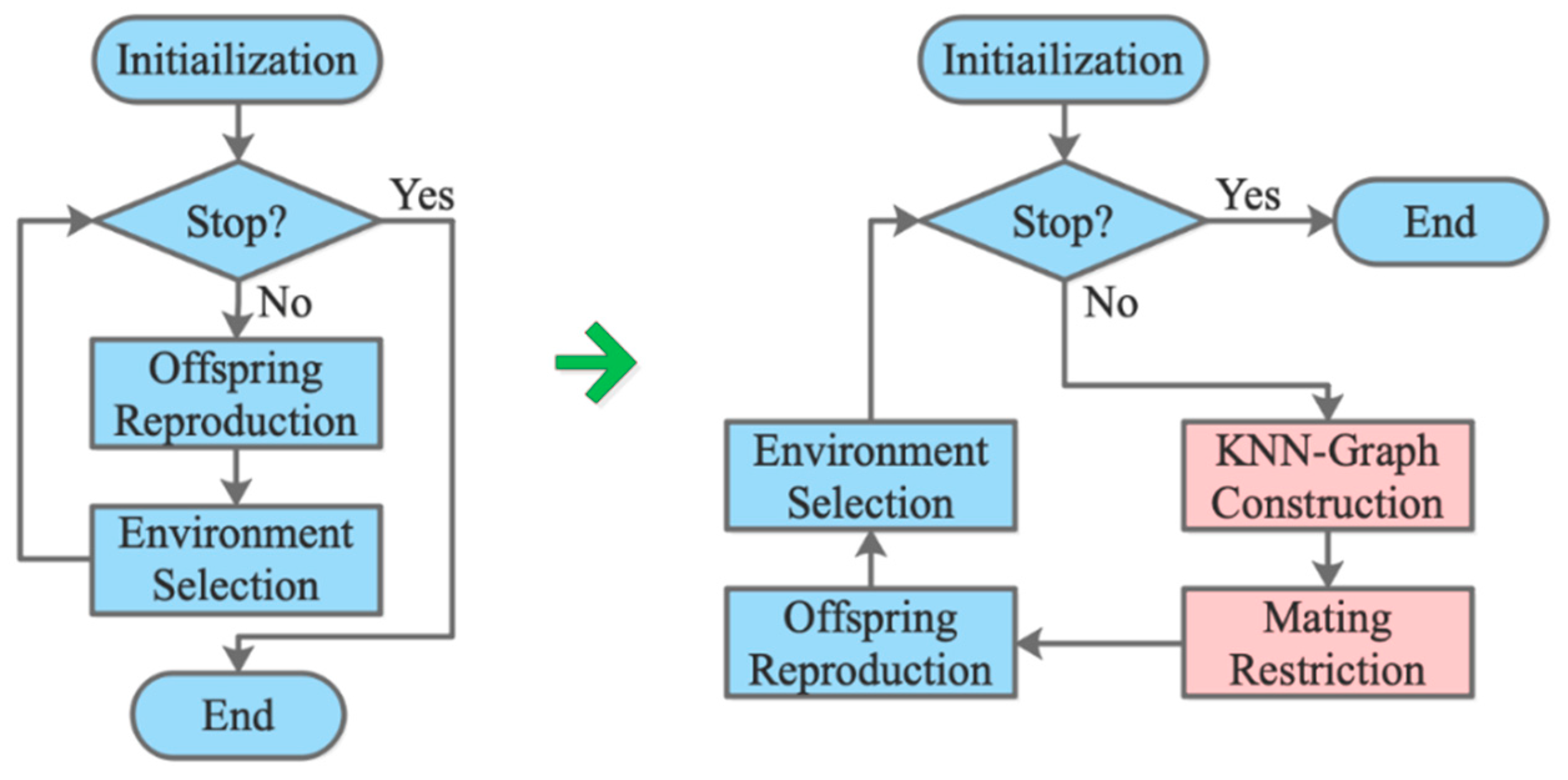
3.3. Proposed Algorithm Based on KNN-Graph

A general MOEA framework is shown in the left part of Figure 5. To improve the search efficiency, we propose to use a KNN-Graph to learn the population structure and guide the new solution generation. The new algorithm framework is shown in the right part of Figure 5 The pseudo code of the new algorithm, which is called MOEA-KG, is presented in Algorithm 1. Some comments about the algorithm are given as follows.

Algorithm 1 MOEA—KG

Input:   n: Population size   Time: The maximum number of generations   K: Number of neighbors-graph  $\beta$: probability of mating restriction Output:   $\mathit{P}\mathit{o}{\mathit{p}}_{\mathit{T}\mathit{i}\mathit{m}\mathit{e}}$: Final population Population initialization, $\mathit{P}\mathit{o}{\mathit{p}}_{\mathbf{0}}=\left\{{\mathit{x}}^{\mathbf{1}},\dots ,{\mathit{x}}^{\mathit{n}}\right\}$ for t = 1: Time do Set an archive population $A$ = $\varnothing$, construct KNN-Graph with $P_t$ foreach$\mathit{p}\in \mathit{P}\mathit{o}{\mathit{p}}_{\mathit{t}-1}$do    $\mathit{Q}=\{\begin{array}{c}\mathit{K}\mathit{N}\mathit{N}\left(\mathit{p}\right)\mathit{i}\mathit{f}\mathit{r}\mathit{a}\mathit{n}\mathit{d}()<\mathit{\beta }\\ \mathit{P}\mathit{o}{\mathit{p}}_{\mathit{t}-\mathbf{1}}\mathit{o}\mathit{t}\mathit{h}\mathit{e}\mathit{r}\mathit{w}\mathit{i}\mathit{s}\mathit{e}\end{array}$, where $rand()$ produces a random number with uniform distribution between [0,1] $\mathit{y}=\mathit{S}\mathit{o}\mathit{l}\mathit{G}\mathit{e}\mathit{n}\left(\mathit{Q},\mathit{p},@DE\right)$    $\mathit{A}=\mathit{A}{{\displaystyle \cup }}^{}\left\{\mathit{y}\right\}$   endforeach $\mathit{P}\mathit{o}{\mathit{p}}_{\mathit{t}-\mathbf{1}}=\mathit{A}{{\displaystyle \cup }}^{}\mathit{P}\mathit{o}{\mathit{p}}_{\mathit{t}-\mathbf{1}}$   $\mathit{P}\mathit{o}{\mathit{p}}_{\mathit{t}}=\mathit{E}\mathit{n}\mathit{v}\mathit{S}\mathit{e}\mathit{l}\left(\mathit{P}\mathit{o}{\mathit{p}}_{\mathit{t}-\mathbf{1}},\mathrm{n}\right)$ endfor Return$\mathit{P}\mathit{o}{\mathit{p}}_{\mathit{T}\mathit{i}\mathit{m}\mathit{e}}$

Initialization (line 1): Randomly generate an initial population $\mathit{P}\mathit{o}{\mathit{p}}_{\mathbf{0}}=\left\{{\mathit{x}}^{\mathbf{1}},\dots ,{\mathit{x}}^{\mathit{n}}\right\}$.

Offspring reproduction (lines 3–7): Firstly, an archive population is set, then the KNN-Graph is established. With the obtained neighbor relationship, solutions are mated with similar solutions by mating restrictions probability. The differential evolution (DE) operator is used to generate new individuals, and then the polynomial mutation method is performed with the new trail solutions (line 6). The mating restriction probability β is used to balance the local exploitation and global exploration of the population.

The details of this reproduction operator are given in Algorithm 2. Three individuals are selected from the mating pool. Through difference operator, the algorithm will get a new individual $\mathit{q}$. Then $\mathit{q}$ will mate with the parent individual $\mathit{x}$ with probability $\mathit{C}\mathit{R}$ to produce the individual $\mathit{u}$, which is returned as a new candidate solution.

Algorithm 2 Reproduction Operator: $\mathit{y}=\mathit{S}\mathit{o}\mathit{l}\mathit{G}\mathit{e}\mathit{n}\left(\mathit{Q},\mathit{x},@DE\right)$

Input:   $\mathit{Q}$: mating pool   $\mathit{p}$: a parent solution   $@DE$: scaling operator $F$; crossover probability $CR$ Output:   $\mathit{y}$: a new candidate solution Randomly select ${\mathit{q}}^{\mathbf{1}}$, ${\mathit{q}}^{\mathbf{2}}$, ${\mathit{q}}^{\mathbf{3}}$, from $\mathit{Q}$ $\mathit{q}={\mathit{q}}^{\mathbf{1}}+F\times \left({\mathit{q}}^{\mathbf{2}}\mathbf{-}{\mathit{q}}^{\mathbf{3}}\right)$ $\mathit{y}=\mathit{p}$ for i =1:$\left|\mathit{y}\right|$ do $if\left(\mathit{rand}()<CR\right){\mathit{y}}_{\mathit{i}}={\mathit{q}}_{\mathit{i}}$ endfor Return$\mathit{y}$

Environment selection (line 10): different environment selection approaches can be embedded with the proposed approach. To indicate the proposed offspring reproduction method, the SPEA2 [21] and SMS-EMOA [37] environment selection paradigms were used to update the population. The SMS-EMOA and SPEA2 environment selection operators are shown in Algorithms 3 and 4, respectively.

Algorithm 3 shows the environment selection operator of SMS-EMOA. First, we obtain the Pareto front (PF) of the input data through fast non-dominated sorting. Then, we find the individuals with the lowest hypervolume contribution $\left[{\Delta }_{\mathit{s}}\left(\mathit{x},R_v\right)\right]$ in the worst frontier and remove them. Finally, the remaining individuals are returned. Non-dominated sorting is a sorting algorithm for multi-dimensional arrays. Its definition and specific steps are from the literature [38]. The calculation method of $\left[{\Delta }_{\mathit{s}}\left(\mathit{x},R_v\right)\right]$ is referred to [37].

Algorithm 3 Environment Selection of SMS—EMOA: $\mathit{P}\mathit{o}{\mathit{p}}_{\mathit{t}}=\mathit{EnvSel}\left(\mathit{P}\mathit{o}{\mathit{p}}_{\mathit{t}-\mathbf{1}},n\right)$

Input:   $\mathit{P}\mathit{o}{\mathit{p}}_{\mathit{t}-\mathbf{1}}$: a combination of the old population and the newly generated solutions   n: population size Output:   $\mathit{P}\mathit{o}{\mathit{p}}_{\mathit{t}}$: the new population $\left\{R_1,\dots ,R_v\right\}\leftarrow \mathit{Fast}-\mathit{Non}-\mathit{Dominated}-\mathit{Sorting}\left\{\mathit{P}\mathit{o}{\mathit{p}}_{\mathit{t}-\mathbf{1}}\right\}$ $\mathit{r}\leftarrow \mathit{argmi}{\mathit{n}}_{\mathit{x}\in R_v}\left[{\Delta }_{\mathit{s}}\left(\mathit{x},R_v\right)\right]$ $\mathit{P}\mathit{o}{\mathit{p}}_{\mathit{t}}=\mathit{A}{\displaystyle \cup }\mathit{P}\mathit{o}{\mathit{p}}_{\mathit{t}-\mathbf{1}}\backslash \left\{\mathit{r}\right\}$ Return$\mathit{P}\mathit{o}{\mathit{p}}_{\mathit{t}}$

Algorithm 4 shows the environment selection operator of SPEA2. First, the next generation population ${\mathit{P}}_{\mathit{t}}$ is left blank. Then, the non-dominated individuals of the input data, namely the Pareto Set (PS), will be added to the next-generation population individuals. If the population size is larger than the target number N, individuals with higher density values will be removed. If the population size is less than N, continue to add Pareto Set to the ${\mathit{P}}_{\mathit{t}}$. The detailed process of the algorithm is referred to [21].

Algorithm 4 Environment Selection of SPEA2: $\mathit{P}\mathit{o}{\mathit{p}}_{\mathit{t}}=\mathit{E}\mathit{n}\mathit{v}\mathit{S}\mathit{e}\mathit{l}\left(\mathit{P}\mathit{o}{\mathit{p}}_{\mathit{t}-\mathbf{1}},n\right)$

Input:   $\mathit{P}\mathit{o}{\mathit{p}}_{\mathit{t}-\mathbf{1}}$: a combination of the old population and the newly generated solutions   n: population size Output:   $\mathit{P}\mathit{o}{\mathit{p}}_{\mathit{t}}$: the new population $\mathit{P}\mathit{o}{\mathit{p}}_{\mathit{t}}=\varnothing$ $\mathit{P}\mathit{o}{\mathit{p}}_{\mathit{t}}\leftarrow \mathit{N}\mathit{o}\mathit{n}-\mathit{dominant}\mathit{individual}\mathit{choice}\left\{\mathit{P}\mathit{o}{\mathit{p}}_{\mathit{t}-\mathbf{1}}\right\}$ $if\mathit{P}\mathit{o}{\mathit{p}}_{\mathit{t}}$≥n $\mathit{P}\mathit{o}{\mathit{p}}_{\mathit{t}}\leftarrow \mathit{truncate}\mathit{the}\mathit{population}\mathit{P}\mathit{o}{\mathit{p}}_{\mathit{t}}$ $else$ $\mathit{P}\mathit{o}{\mathit{p}}_{\mathit{t}}\leftarrow \mathit{select}\mathit{the}$superior individual from$\left\{\mathit{P}\mathit{o}{\mathit{p}}_{\mathit{t}-\mathbf{1}}\right\}\backslash \mathit{P}\mathit{o}{\mathit{p}}_{\mathit{t}}$ Return$\mathit{P}\mathit{o}{\mathit{p}}_{\mathit{t}}$

4. Experimental Study

4.1. Performance Index

In order to measure the convergence and diversity of the proposed algorithm, we use two performance indicators: Inverted Generational Distance (IGD) [39] and Hypervolume (HV) [40]. Both IGD and HV can simultaneously evaluate the diversity and convergence of algorithms, and have good intuitiveness.

(1)

Inverted Generational Distance (IGD)

For an obtained population P and a reference population P*, IGD is defined as

$$IGD\left(P^{\ast },P\right)=\frac{{{\displaystyle \sum }}_{x^{\ast }ϵP^{\ast }}d\left(x^{\ast },P^{\ast }\right)}{\left|P^{\ast }\right|}$$

(11)

where $d\left(x^{\ast },P^{\ast }\right)$ is the minimum distance between the target point $x^{\ast }$ and all points in the set point $P$. $\left|P^{\ast }\right|$ is the number of points in $P^{\ast }$. The larger IGD, the more ideal the frontier P is.

(2)

Hypervolume (HV)

For an obtained population P and a reference point r, HV is defined as

$$HV\left(P,r\right)=VOL\left\{\begin{array}{c}\mathrm{Y}\\ xϵP\end{array}\left[f_1\left(x\right),r_1\right]\times \dots \left[f_m\left(x\right),r_m\right]\right\}$$

(12)

where $r=\left(r_1,\dots ,r_m\right)$ is a reference point dominated by any target point in the target space.$VOL()$ is the Lebesgue measurement. The HV index measures the volume of the target space surrounded by all points in the boundary with $r$. The larger the value of the HV index, the more widely the Pareto solution set obtained can cover its real front end, and the better the scalability and distribution of the algorithm.

4.2. Comparison and Analysis of KNN-Graph Based Operator on General Problems

In order to verify the effectiveness of the KNN-Graph based reproduction operator, we introduce it into the two MOEAs, i.e., SMS-EMOA and SPEA2, and get two new algorithms, called SMS-EMOA-KG and SPEA2-KG respectively. In addition to comparing with the original algorithms, we also conduct a comparative study with some state-of-the-art multi-objective evolutionary algorithms MOEA/D-DE [24], RM-MEDA [41], IM-MOEA [42], and SMEA [43]. In order to have a fair comparison, the differential evolution operator is used to replace the reproduction operators used in the original SMS-EMOA and SPEA2. The parameters required for each comparison algorithm are shown in

Table 1. Experimental parameter setting.

Instance	Parameter Settings
Public parameter	Population size N: 100
	The maximum number of evolutions T: 300
	Number of operations: 30
DE operator	$F=0.5,CR=1$, $P_m=\frac{1}{\mathrm{n}},{ŋ}_m=20$
MOEA/D-DE	Neighborhood size NS: 5
	Parent selection probability $\beta$: 0.9
	Number of new solutions nr: 0.2
IM-MOEA	Number of reference vectors K: 10
RM-MEDA	Number of clusters K: 5
	Number of clustering iterations: 50
	Sampling expansion rate: 0.25
SMEA	Initial learning rate ${\tau }_0$: 0.9
	Neighbor mating pool size H: 10
	Mating limit probability $\beta$: 0.9
Proposed MOEA	Nearest neighbor size K: 10
	Gaussian similarity bandwidth σ: 1
	Mating restriction probability β: 0.7

. In practical engineering applications, because the actual PS or PF is often unknown, when choosing an algorithm, it is often biased toward an optimization algorithm that can solve complex rule structures. Therefore, this paper chooses GLT1-GLT6 [42] with complex PFs and UF1-UF10 [43] with complex PSs as the test sets. The reference point for calculating HV is $r=1.1\times \max PF\left[f_1,\dots ,f_m\right]$.

Table 2. The statistical results obtained by two SMS-EMOA variations. The numbers outside the parentheses indicate the average of 30 experiments. The numbers in () indicate the variance of 30 experiments.

Instance.	SMS-EMOA-DE	SMS-EMOA-KG
	IGD
GLT1	1.4693 × 10−1 (2.12 × 10−2) −	1.8742 × 10−3 (6.57 × 10−5)
GLT2	9.0037 × 10−1 (5.12 × 10−1) −	2.9636 × 10−2 (8.15 × 10−4)
GLT3	2.0581 × 10−1 (4.16 × 10−2) −	5.7233 × 10−3 (1.61 × 10−3)
GLT4	2.2679 × 10−1 (3.10 × 10−2) −	2.9274 × 10−2 (4.57 × 10−2)
GLT5	1.8252 × 10−1 (6.64 × 10−2) −	6.5220 × 10−2 (5.92 × 10−3)
GLT6	3.1223 × 10−1 (2.64 × 10−1) =	1.2574 × 10−1 (7.16 × 10−2)
+/−/=	0/5/1	-

and

Table 3. The statistical results obtained by two SPEA2 variations. The numbers outside the parentheses indicate the average of 30 experiments. The numbers in () indicate the variance of 30 experiments.

Instance	SPEA2-DE	SPEA2-KG
	IGD
GLT1	1.3775 × 10−1 (2.60 × 10−2) −	2.6329 × 10−3 (1.27 × 10−4)
GLT2	5.9186 × 10−1 (3.30 × 10−1) −	3.0671 × 10−2 (1.21 × 10−3)
GLT3	1.6531 × 10−1 (5.41 × 10−2) −	8.3622 × 10−3 (5.54 × 10−3)
GLT4	2.1576 × 10−1 (3.18 × 10−2) −	6.1220 × 10−3 (1.26 × 10−4)
GLT5	5.6489 × 10−2 (2.20 × 10−2) =	4.2734 × 10−2 (1.94 × 10−3)
GLT6	1.9984 × 10−1 (2.66 × 10−1) =	7.9232 × 10−2 (6.32 × 10−2)
+/−/=	0/4/2	-

present the results obtained by the two algorithms SMS-EMOA-DE and SPEA-DE that use differential evolution operators, and SMS-EMOA-KG and SPEA2-KG that integrate reproduction operators based on KNN-Graph. We used the Wilcoxon rank sun test to compare experimental results, where ‘+’,‘−’,‘=’ in Table 2 and Table 3 indicate the value obtained by the algorithm with KNN is greater than, smaller than, or similar than that obtained by the traditional algorithm based version at a 95% significance level. The statistical results of the average IGD values obtained by computing the two sets of test sets 30 times independently are shown in these two tables. It can be seen from the tables that compared to the original algorithms, the improved algorithms with the KNN-Graph based operator, i.e., SMS-EMOA-KG and SPEA2-KG, can obtain better values in the test set GLT1−6. From the results of the Wilcoxon rank sum test, SMS-EMOA-KG achieved five better values and one similar IGD average index value, and SPEA2-KG obtains four better values and two similar IGD average index values. Through the analysis of the above statistical results, we can see that the algorithms with the KNN-Graph based reproduction operator can greatly improve the performance of the original algorithms.

Table 4. The statistical results obtained by six comparison algorithms. The numbers outside the parentheses indicate the average of 30 experiments. The numbers in () indicate the variance of 30 experiments. The number in [] indicates the ranking of the performance of the 6 algorithms. The number one algorithm is Shaded.

Instance	MOEA/D-DE	RM-MEDA	IMMOEA	SMEA	SMS-EMOA-KG	SPEA2-KG
	IGD
GLT1	3.6774 × 10−3 (2.61 × 10−5) [3]	4.2663 × 10−3 (1.23 × 10−3) [4]	2.2247 × 10−2 (2.71 × 10−3) [6]	1.4459 × 10−2 (9.85 × 10−3) [5]	2.4453 × 10−3 (3.71 × 10−3) [1]	2.9421 × 10−3 (1.39 × 10−3) [2]
GLT2	3.2232 × 10−1 (3.61 × 10−2) [4]	3.2144 × 10−2 (1.17 × 10−3) [3]	3.8994 × 10−1 (8.99 × 10−2) [6]	3.2742 × 10−2 (1.92 × 10−3) [5]	2.9920 × 10−2 (4.30 × 10−4) [1]	3.0933 × 10−2 (6.18 × 10−4) [2]
GLT3	2.1921 × 10−2 (3.85 × 10−3) [3]	1.3770 × 10−2 (1.15 × 10−2) [2]	1.1284 × 10−1 (3.50 × 10−2) [6]	3.8291 × 10−2 (4.23 × 10−3) [5]	5.2081 × 10−3 (2.01 × 10−4) [1]	2.3559 × 10−2 (3.60 × 10−2) [4]
GLT4	9.5931 × 10−3 (5.31 × 10−5) [4]	6.2274 × 10−3 (2.06 × 10−4) [2]	2.7685 × 10−2 (8.94 × 10−3) [5]	4.8657 × 10−2 (8.25 × 10−2) [6]	8.1160 × 10−3 (2.05 × 10−3) [3]	6.2081 × 10−3 (1.85 × 10−3) [1]
GLT5	1.37291 × 10−1 (1.10 × 10−3) [6]	5.1563 × 10−2 (2.09 × 10−3) [2]	7.7029 × 10−2 (4.17 × 10−3) [5]	7.5621 × 10−2 (6.99 × 10−3) [4]	6.8898 × 10−2 (3.05 × 10−3) [3]	4.3850 × 10−2 (1.26 × 10−3) [1]
GLT6	8.3443 × 10−2 (6.88 × 10−3) [6]	5.2764 × 10−2 (7.66 × 10−4) [1]	7.3297 × 10−2 (1.00 × 10−3) [2]	8.0387 × 10−2 (4.19 × 10−3) [5]	7.6088 × 10−1 (6.68 × 10−2) [3]	7.6102 × 10−2 (2.03 × 10−2) [4]
UF1	8.6461 × 10−2 (2.28 × 10−2) [3]	9.5013 × 10−2 (7.04 × 10−3) [5]	9.7365 × 10−2 (7.44 × 10−3) [6]	8.2864 × 10−2 (1.18 × 10−2) [2]	8.1144 × 10−2 (2.95 × 10−2) [1]	9.2310 × 10−2 (4.60 × 10−2) [4]
UF2	3.9917 × 10−2 (2.25 × 10−2) [5]	3.3042 × 10−2 (6.31 × 10−3) [3]	3.8612 × 10−2 (9.89 × 10−3) [4]	5.2072 × 10−2 (5.48 × 10−3) [6]	3.0435 × 10−2 (6.83 × 10−3) [1]	3.0879 × 10−2 (4.21 × 10−3) [2]
UF3	2.0154 × 10−1 (7.46 × 10−2) [6]	1.0445 × 10−1 (6.51 × 10−2) [1]	1.3722 × 10−1 (1.54 × 10−2) [2]	1.6362 × 10−1 (1.00 × 10−2) [5]	1.6010 × 10−1 (2.10 × 10−2) [3]	1.6331 × 10−1 (2.89 × 10−2) [4]
UF4	9.6573 × 10−2 (8.07 × 10−3) [5]	1.0032 × 10−1 (8.35 × 10−3) [6]	8.7950 × 10−2 (3.88 × 10−3) [4]	7.5709 × 10−2 (1.02 × 10−2) [2]	7.2361 × 10−2 (8.24 × 10−3) [1]	7.6709 × 10−2 (1.21 × 10−2) [3]
UF5	9.3052 × 10−1 (2.04 × 10−1) [1]	1.2277 (4.80 × 10−1) [4]	1.1768(1.99 × 10−1) [2]	1.3446 (2.37 × 10−1) [5]	1.1961 (2.40 × 10−1) [3]	1.3565 (2.28 × 10−1) [6]
UF6	3.2487 × 10−1 (9.43 × 10−2) [2]	4.8169 × 10−1 (9.66 × 10−2) [5]	2.9028 × 10−1 (4.60 × 10−2) [1]	5.1783 × 10−1 (7.30 × 10−2) [6]	4.0794 × 10−1 (4.58 × 10−2) [3]	4.2120 × 10−1 (4.63 × 10−2) [4]
UF7	1.3295 × 10−1 (2.07 × 10−1) [6]	6.6774 × 10−2 (1.24 × 10−2) [3]	1.1074 × 10−1 (8.74 × 10−2) [5]	4.6647 × 10−2 (2.15 × 10−2) [2]	7.1989 × 10−2 (1.10 × 10−1) [4]	4.5395 × 10−2 (1.30 × 10−2) [1]
UF8	3.8785 × 10−1 (2.15 × 10−2) [5]	3.6714 × 10−1 (3.99 × 10−2) [3]	3.7651 × 10−1 (6.40 × 10−3) [4]	3.5880 × 10−1 (9.20 × 10−2) [2]	3.3582 × 10−1 (7.13 × 10−2) [1]	6.6597 × 10−1 (1.46 × 10−1) [6]
UF9	3.2838 × 10−1 (8.93 × 10−2) [3]	4.9841 × 10−1 (1.13 × 10−1) [5]	3.9872 × 10−1 (4.10 × 10−2) [4]	2.4864 × 10−1 (1.00 × 10−1) [1]	3.1443 × 10−1 (9.29 × 10−2) [2]	9.5494 × 10−1 (2.02 × 10−1) [6]
UF10	1.0303(1.13 × 10−1) [2]	2.6789(2.80 × 10−1) [5]	3.1850 × 10−1 (7.19 × 10−3) [1]	2.7334(2.43 × 10−1) [6]	1.5658(1.44 × 10−1) [3]	2.5390(4.22 × 10−1) [4]
	HV
GLT1	5.6182 × 10−1 (3.14 × 10−4) [4]	5.6428 × 10−1 (9.64 × 10−3) [3]	5.0380 × 10−1 (5.95 × 10−3) [6]	5.2400 × 10−1 (2.39 × 10−2) [5]	5.6610 × 10−1 (2.10 × 10−2) [1]	5.6588 × 10−1 (9.46 × 10−3) [2]
GLT2	9.5478 (2.78 × 10−2) [5]	9.8375 (1.07 × 10−2) [4]	8.7650 (3.02 × 10−1) [6]	9.8701 (6.89 × 10−3) [2]	9.9096 (4.73 × 10−4) [1]	9.8408 (6.59 × 10−3) [3]
GLT3	1.1535 (6.90 × 10−4) [5]	1.1559 (9.23 × 10−4) [3]	1.1446 (3.30 × 10−3) [6]	1.1552 (4.69 × 10−4) [4]	1.1588 (8.23 × 10−5) [1]	1.1560 (3.36 × 10−3) [2]
GLT4	1.4070 (4.89 × 10−4) [3]	1.4080 (9.38 × 10−4) [2]	1.3709 (1.32 × 10−2) [5]	1.3791 (5.15 × 10−2) [4]	1.2153 (3.89 × 10−1) [6]	1.4081 (9.02 × 10−4) [1]
GLT5	1.2656 (9.88 × 10−4) [3]	1.2679 (3.01 × 10−3) [2]	1.2580 (1.42 × 10−3) [4]	1.2382 (6.38 × 10−3) [6]	1.2560 (4.47 × 10−3) [5]	1.2817 (1.49 × 10−3) [1]
GLT6	1.2502 (4.76 × 10−3) [2]	1.2591 (1.33 × 10−3) [1]	1.2357 (4.54 × 10−3) [3]	1.2316 (1.11 × 10−2) [4]	1.1409 (8.06 × 10−2) [5]	1.1284 (4.31 × 10−2) [6]
UF1	7.1640 × 10−1 (4.06 × 10−2) [3]	7.0686 × 10−1 (1.44 × 10−2) [5]	7.3922 × 10−1 (2.21 × 10−2) [1]	7.2245 × 10−1 (2.18 × 10−2) [2]	7.0417 × 10−1 (5.24 × 10−2) [6]	7.1295 × 10−1 (6.68 × 10−2) [4]
UF2	8.1799 × 10−1 (2.73 × 10−2) [5]	8.2188 × 10−1 (5.42 × 10−3) [4]	8.2465 × 10−1 (7.17 × 10−3) [3]	7.9779 × 10−1 (7.70 × 10−3) [6]	8.2827 × 10−1 (8.18 × 10−3) [1]	8.2650 × 10−1 (5.58 × 10−3) [2]
UF3	5.3662 × 10−1 (1.07 × 10−1) [6]	6.9713 × 10−1 (9.91 × 10−2) [1]	6.3494 × 10−1 (3.75 × 10−2) [2]	6.2063 × 10−1 (1.28 × 10−2) [3]	6.0526 × 10−1 (4.27 × 10−2) [4]	6.0525 × 10−1 (4.62 × 10−2) [5]
UF4	3.7932 × 10−1 (1.21 × 10−2) [5]	3.7227 × 10−1 (1.28 × 10−2) [6]	3.9313 × 10−1 (8.06 × 10−3) [4]	3.9360 × 10−1 (1.55 × 10−2) [3]	3.9765 × 10−1 (1.14 × 10−2) [1]	3.9606 × 10−1 (2.02 × 10−2) [2]
UF5	3.7857 × 10−3 (7.59 × 10−3) [1]	0.0000 (0.00) [2]	0.0000 (0.00) [2]	0.0000 (0.00) [2]	0.0000 (0.00) [2]	0.0000 (0.00) [2]
UF6	2.8723 × 10−1 (1.01 × 10−1) [1]	5.8323 × 10−2 (8.76 × 10−3) [4]	2.6305 × 10−1 (2.56 × 10−2) [2]	6.0804 × 10−2 (3.03 × 10−2) [5]	1.3355 × 10−1 (5.15 × 10−2) [3]	9.7642 × 10−2 (6.55 × 10−2) [6]
UF7	5.5604 × 10−1 (1.76 × 10−1) [5]	5.9038 × 10−1 (2.25 × 10−2) [4]	5.4816 × 10−1 (1.04 × 10−1) [6]	6.2335 × 10−1 (3.72 × 10−2) [2]	6.1029 × 10−1 (1.07 × 10−1) [3]	6.2370 × 10−1 (2.38 × 10−2) [1]
UF8	3.8148 × 10−1 (2.15 × 10−2) [4]	1.9583 × 10−1 (6.27 × 10−2) [5]	4.1458 × 10−1 (9.78 × 10−3) [2]	3.8590 × 10−1 (4.13 × 10−2) [3]	4.2332 × 10−1 (3.34 × 10−2) [1]	2.8157 × 10−2 (2.84 × 10−2) [6]
UF9	5.9709 × 10−1 (1.33 × 10−1) [3]	3.3671 × 10−1 (1.41 × 10−1) [5]	4.4102 × 10−1 (3.11 × 10−2) [4]	7.6286 × 10−1 (5.12 × 10−2) [1]	6.8028 × 10−1 (1.17 × 10−1) [2]	1.3613 × 10−2 (2.82 × 10−2) [6]
UF10	1.0574 × 10−4 (2.59 × 10−4) [2]	0.0000 (0.00) [3]	2.9112 × 10−1 (2.53 × 10−2) [1]	0.0000 (0.00) [3]	0.0000 (0.00) [3]	0.0000 (0.00) [3]
Mean Rank	3.7813	3.375	3.75	3.8125	2.4688	3.3125

shows the results of using the MOEA/D-DE, RM-MEDA, SMEA, SMS-EMOA, NSGA-Ⅱ, and KG-MOEA algorithms to perform 30 independent calculations on the two test sets. In order to obtain a fair comparison result, the average and standard deviation of the IGD and HV index values were counted. As can be seen from the table, compared to the four comparison algorithms MOEA/D-DE, IM-MOEA, RM-MEDA and SMEA, among the 32 best average index values, SMS-EMOA-KG and SPEA2-KG obtained respectively 13 and 6 optimal average index values, occupying more than half of the optimal index values. Based on the average rank values, the algorithms sorted from best to worst are SMS-EMOA-KG, SPEA2-KG, RM-MEDA, IM-MOEA, MOEAD/DE, and SMEA. Compared with the other four comparison algorithms, the algorithms with the KNN-Graph based reproduction operator achieve the best performances on the test sets GLT and UF with complex PS or PF.

The statistical comparison results show that the introduction of the KNN-Graph based reproduction operator has improved the performance of the original algorithm by orders of magnitude. The above comparison results also verify the effectiveness of the KNN-Graph based reproduction operator. We also noticed that SMS-EMOA-KG works slightly better than SPEA2-KG, which is related to the fitness assignment and environment selection method of the algorithm itself.

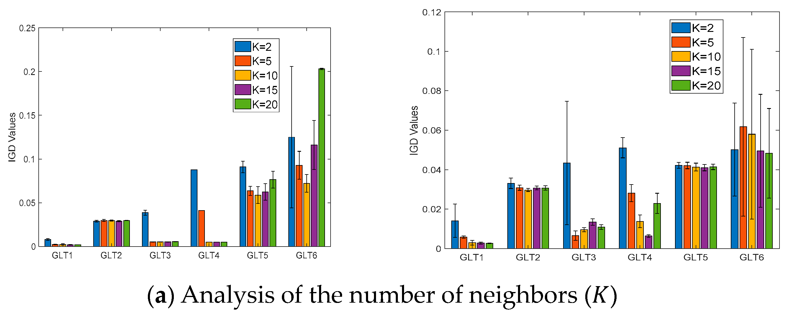
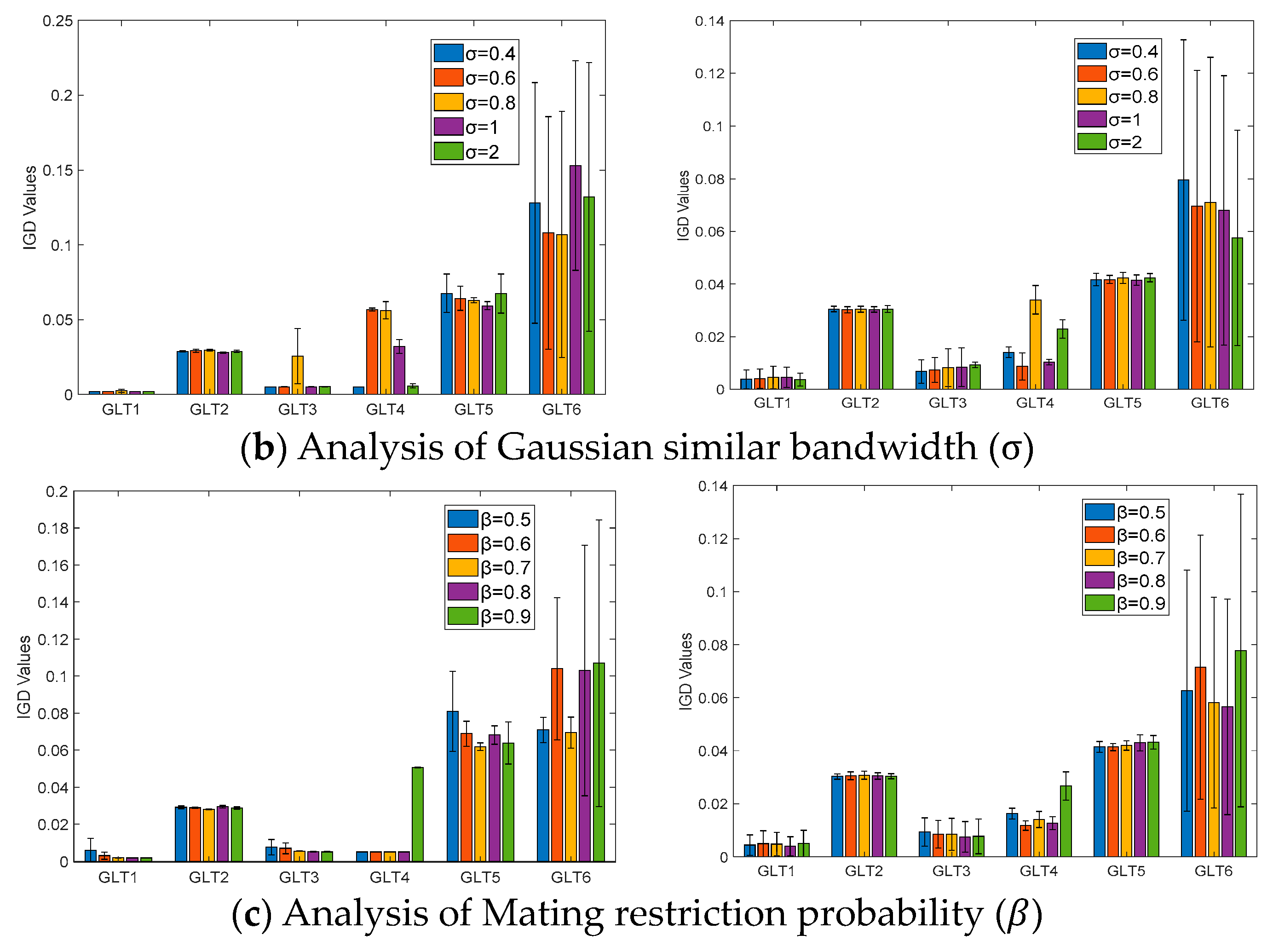
4.3. Parameter Sensitivity

In order to study the influence of control parameters on the KNN-Graph based reproduction operator, the parameter sensitivity analysis is carried out on the main parameters, i.e., the number of neighbors ($K$), the Gaussian similarity bandwidth ($\mathsf{\sigma }$), and the mating restriction probability ($\beta$). We take the GLT test set as an example, and apply SMS-EMOA-KG and SPEA2-KG with different preset parameters to the test problems for 30 times. When setting different values of the above parameters for test experiments, other parameters are the same as in Section 4.2. The experimental results are shown in Figure 6.

From Figure 6, we can find that for SMS-EMOA-KG and SPEA2-KG, when analyzing the number of neighbors $K$, except when $K$ = 2, the overall effect is not good, and the other $K$ values have no effect on the performance of the algorithm. For the five values of Gaussian similarity bandwidth $\mathsf{\sigma }$ and mating restriction probability $\beta$, the two algorithms are not sensitive to their values. In general, the two algorithms that integrate the KNN-Graph based reproduction operator are not very sensitive to parameter settings, which also shows that the KNN-Graph based reproduction operator has better robustness. However, we should also pay attention that the most appropriate parameter value should be related to the problem.

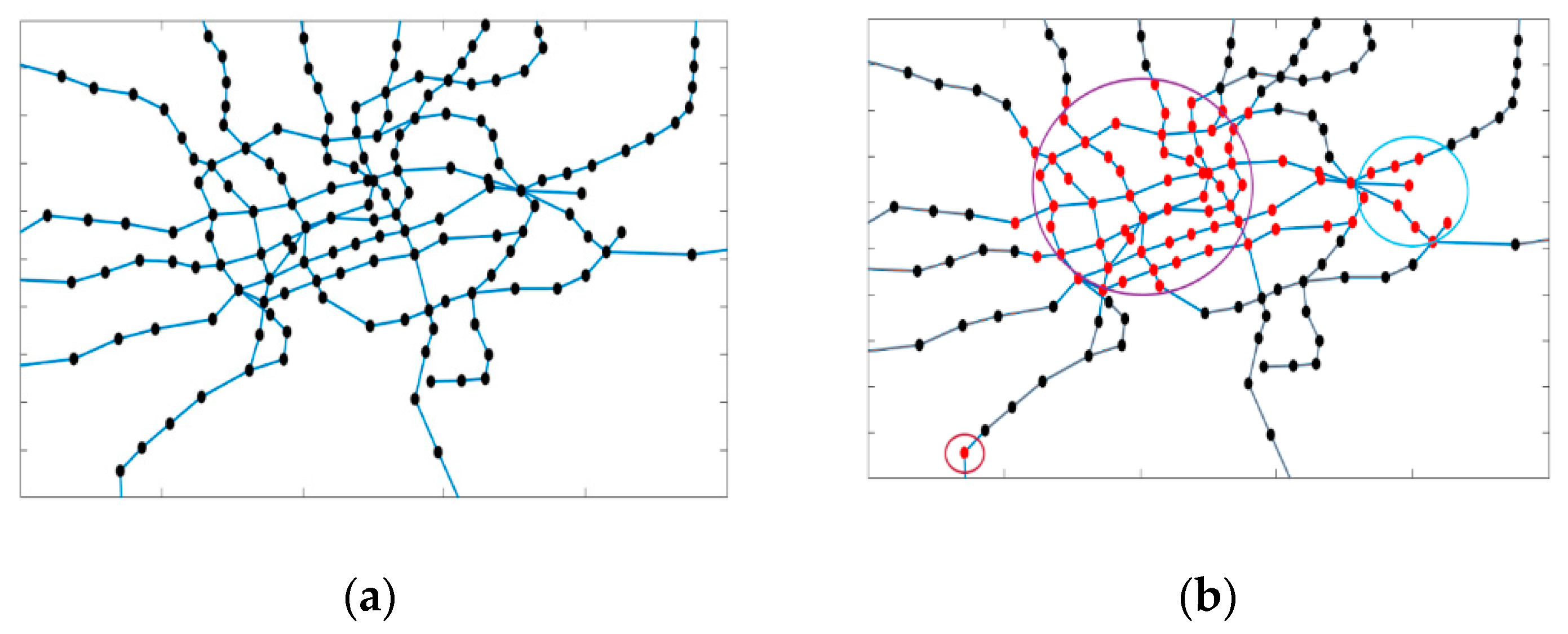
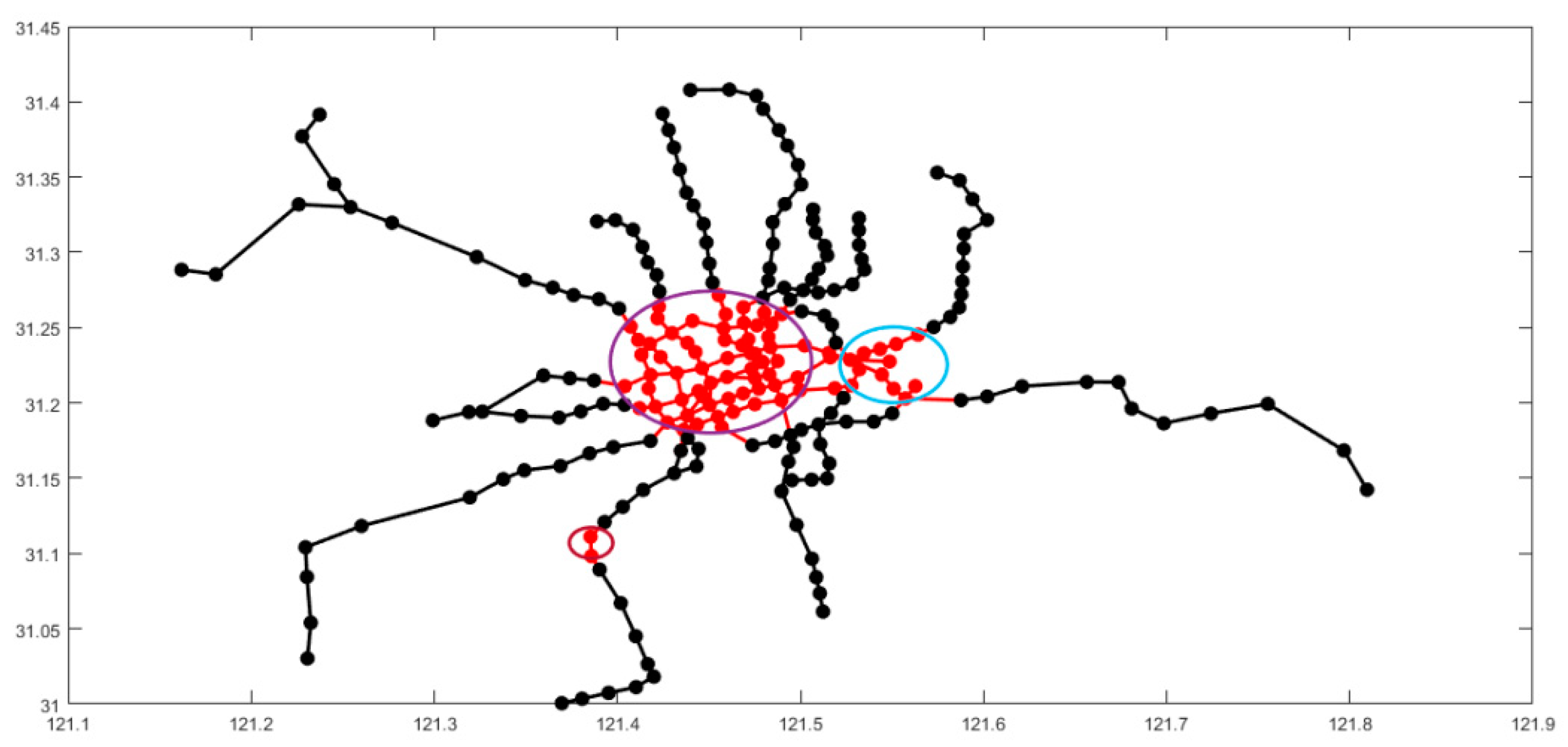
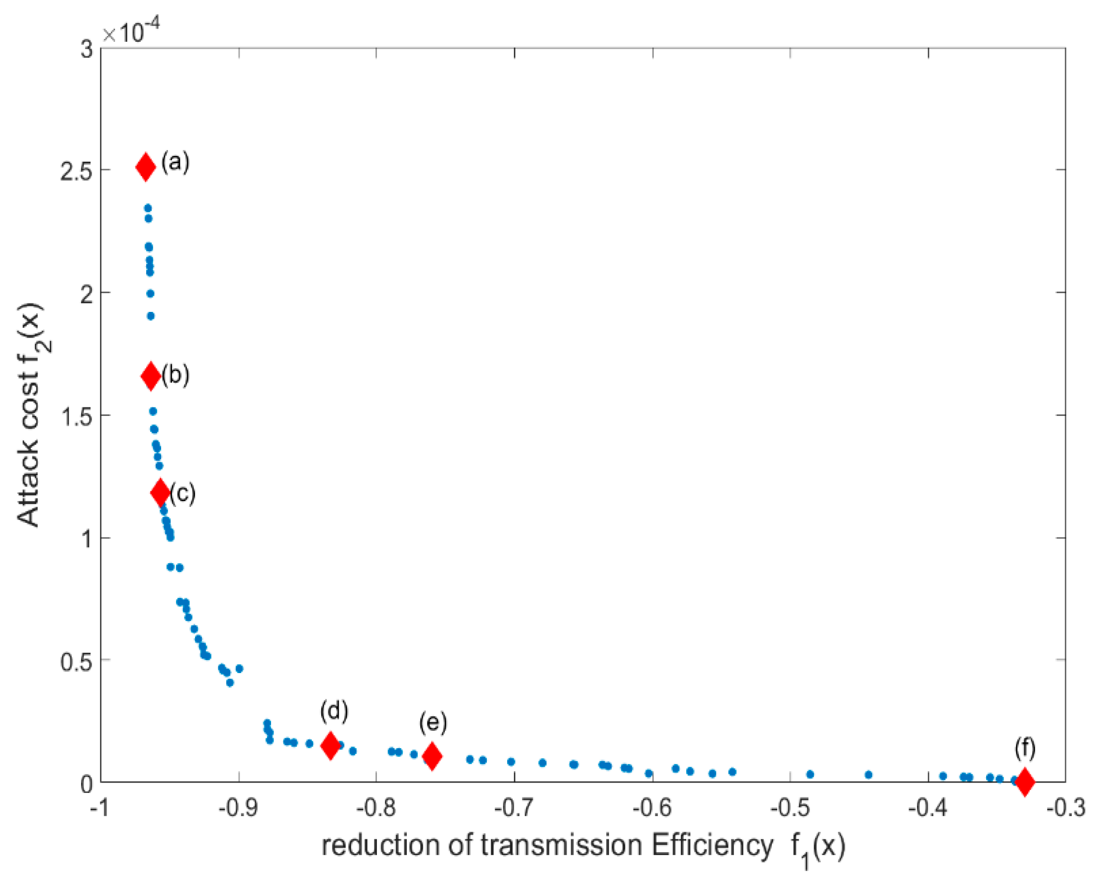
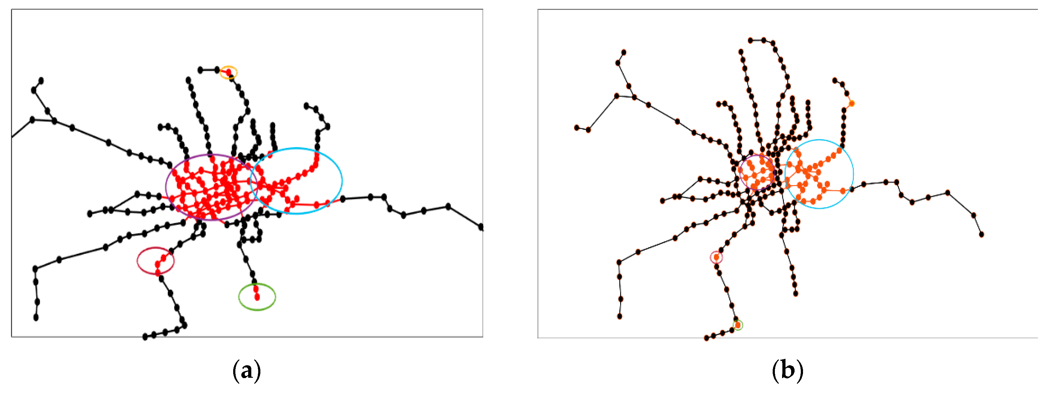
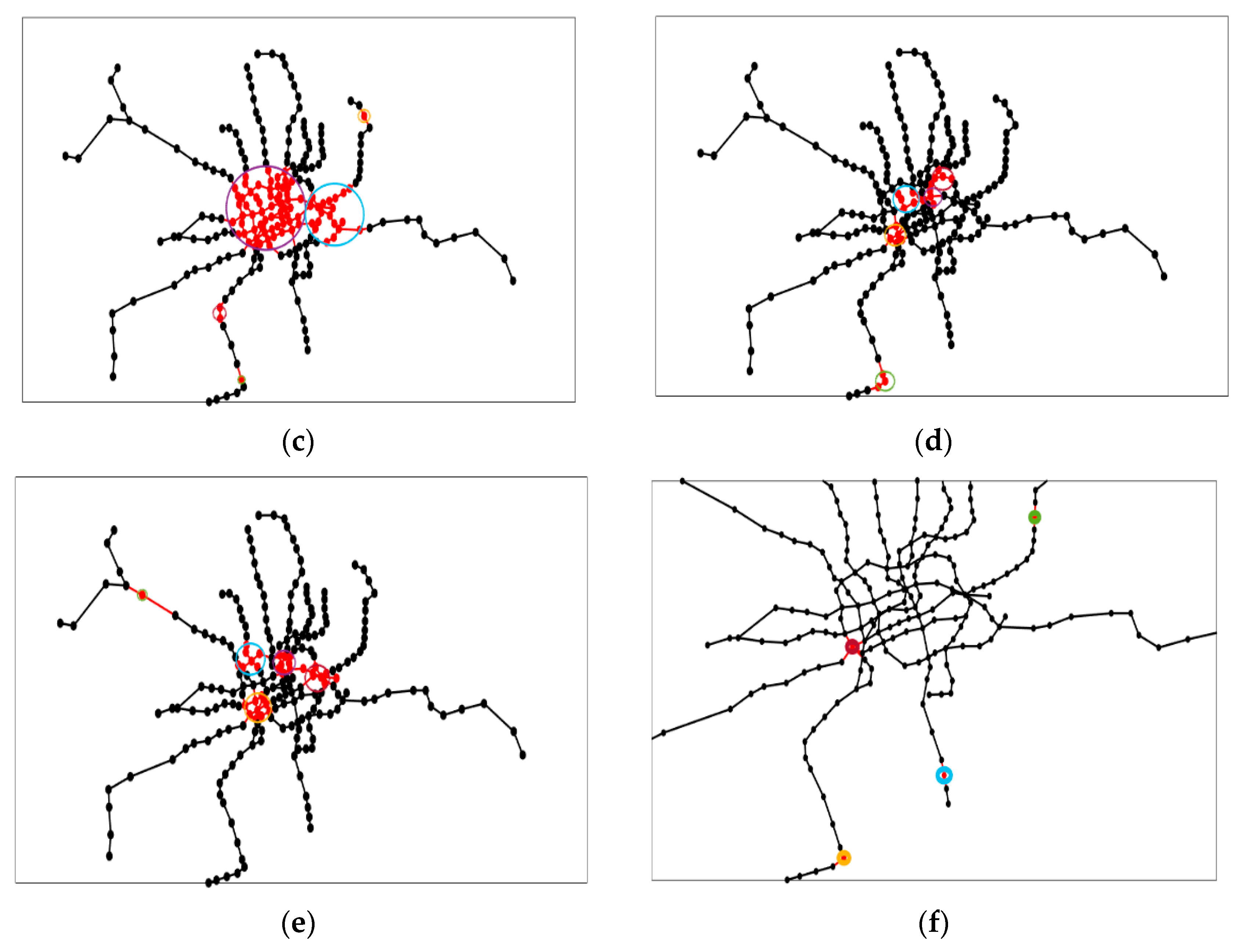
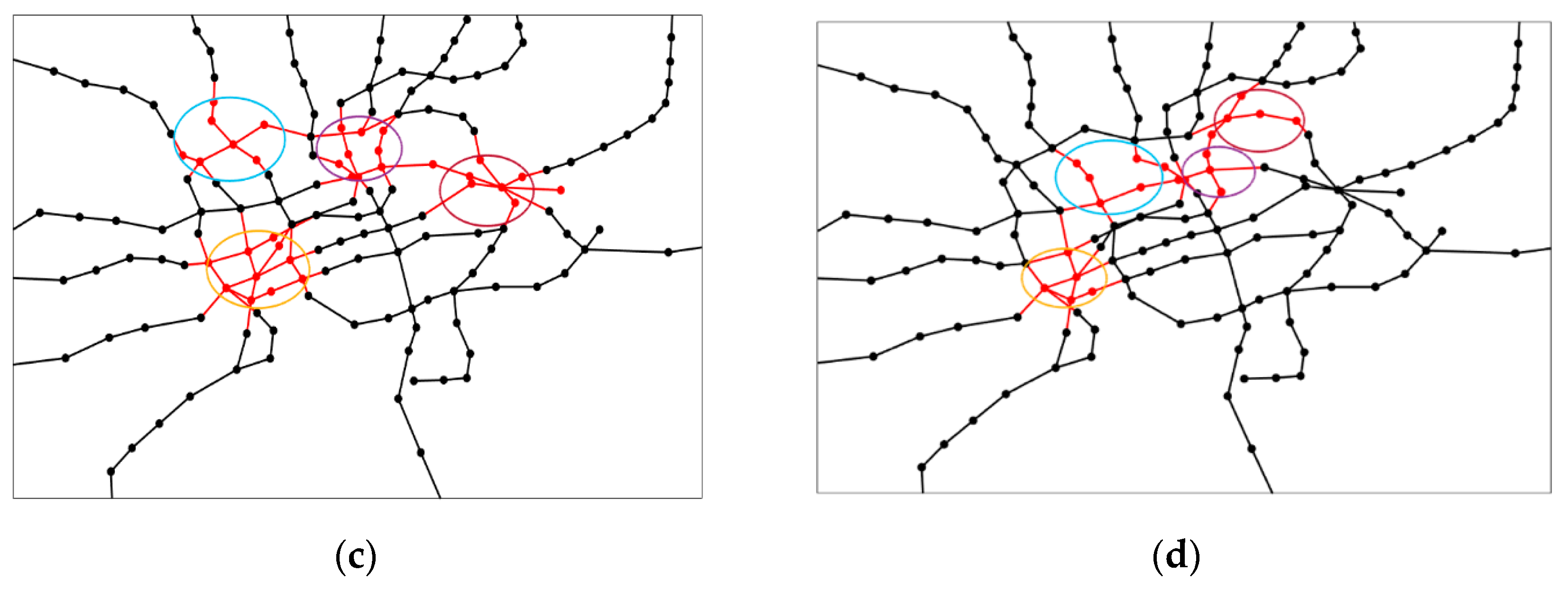
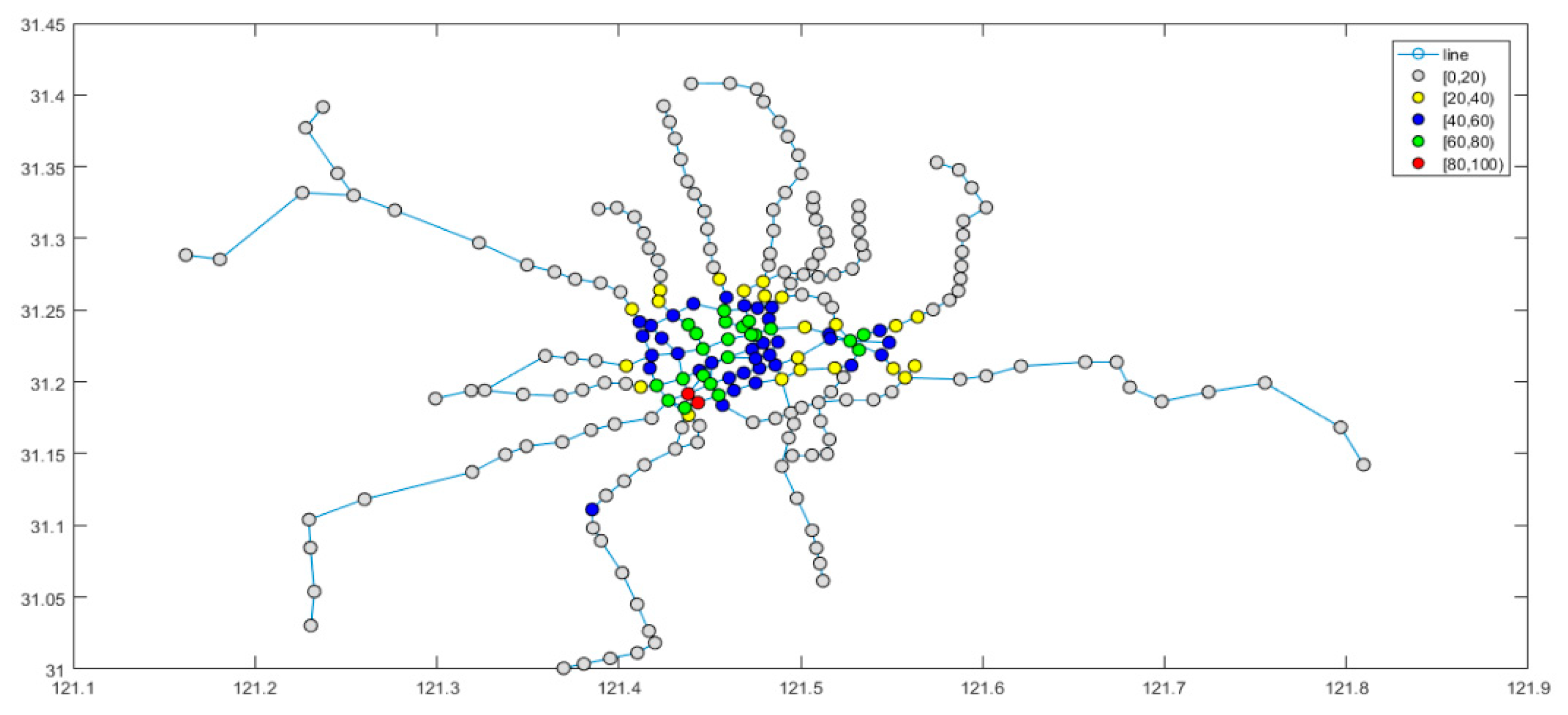
4.4. Results of Network Attack Plan

Combined with the KNN-Graph based reproduction operator, we apply SMS-EMOA-KG to the Shanghai Subway network mentioned in Section 2 and compare the algorithm effect with four traditional algorithms. Choose the attack cost and transportation efficiency drop in Section 2 as the optimization targets. And we set the population size to 100. Finally, we compare the HV value of each algorithm. We ran each algorithm 30 times and showed the average and standard deviation in

Table 5. Mean and Variance of HV after 30 operations of each algorithm.

	SMS-EMOA-KG	MOEA/D-DE	RM-MEDA	IM-MEDA	SMEA
Mean of HV	0.86261	0.8342	0.8357	0.8350	0.8370
Variance of HV	0.0518	0.0519	0.0385	0.0340	0.0763

.

It can be found that the HV value of SMS-EMOA-KG with the KNN-Graph based operator is higher than that of the traditional algorithms, indicating that the overall performance of the algorithm is better.

After iterating for 100 generations with SMS-EMOA-KG, we obtain the final optimized population with 100 attack plans. We show the solutions obtained by the algorithm in a run in Figure 7. To illustrate the attack performances, we choose six reprehensive attacks, the diamonds in Figure 8, and show the attack results in Figure 8.

It is clear that the attack plan (a) and the attack plan (f) only consider objective ${\mathit{f}}_{\mathbf{2}}$ and ${\mathit{f}}_{\mathbf{1}}$ respectively, while attacked plans (b)–(d) consider both optimization objectives. In order to facilitate the observation, we will enlarge the parts of (b)–(d) in Figure 8 and place them in Figure 9 one by one. Figure 8a shows that over-consideration of catch-up effect will result in a large number of ineffective attacks and repeated attacks. Figure 8f shows that excessive consideration of cost will result to smaller attack radius, and surface attacks will degenerate into point attacks. Their results are obviously inferior to the attacked plans in Figure 8a,f. The plans in Figure 8b,c all launched one or two large-scale attacks in the central area of Shanghai, and used small-scale attacks on the peripheral subway lines. The scheme of Figure 8d,e are to launch three or four medium attacks in the center.

As shown in Figure 9, we can find that attacks are mainly concentrated in the central area of the subway network. This area is the central urban area of Xuhui District, Yangpu, and Putuo in Shanghai. Metro stations in these areas have huge passenger flows. Centralized attacks on these areas can quickly paralyze the vast majority of network functions.

For attackers, they are more concerned about how to attack the network. For defenders, they are more concerned about which sites are more vulnerable. We also counted the number of times each site was attacked in these 100 attack scenarios. The results are shown in

Table 6. The attacked times of stations in 100 attack plans.

Attacked Time	0~19	20~39	40~59	60~79	80~100
Count	151	22	35	33	2

. Among them, Xujiahui Station and Shanghai Stadium Station were attacked 81 times and 89 times respectively, indicating that these two sites are extremely important in the network. We plot the attacked time of these stations in Figure 10.

Attack the dense area of the city center with large firepower and use small-scale blasting on the branch line to cut off the network connections. This is exactly the idea displayed by these attack plans, which is consistent with the actual situations.

According to the results obtained by the algorithm, we found the weakest subway stations and urban areas. Sticking to the attacker’s perspective, blasting these areas and stations first can paralyze the network with maximum efficiency. From the perspective of the subway operator, according to the order of the number of attacks, adjusting the security of stations and areas step by step can maximize the normal operation of the subway network.

4.5. Discussion

This paper studies the non-topological indexes commonly used in network vulnerability and uses network transmission efficiency as the vulnerability index of traffic transportation networks. This index not only takes into account the specific functions of the network, but also takes into account the topological and non-topological properties of the network.

At the same time, this paper regards the vulnerability of the network as a confrontation between the attacker and the function of the network itself, thereby introducing evolutionary algorithms to find effective network attack solutions. This is an unprecedented approach since most other studies consider vulnerability only from the function of the network itself, without combining attackers.

In order to improve the convergence of the MOEA algorithm when a new solution reproduction occurs, this paper considers the defects of the cluster-based reproduction operator and uses KNN-Graph to extract the population structure. This new operator improves the convergence of the algorithm at the cost of a small amount of running time.

Our research is based on the specific functions of the network to set its vulnerability index. For example, this article studies the subway network, so traffic transportation is its main function. For other networks with different functions, other reasonable vulnerability indexes should be designed during vulnerability analysis. We believe that reasonable vulnerability indexes can make the vulnerability analysis of the network more consistent with the actual situation.

5. Conclusions and Future Research Directions

This paper first introduces the vulnerability attributes of complex networks. We define the cost and benefit of cyber-attacks and regard the assessment of vulnerability attributes as an attacker’s choice between these two attributes. In this way, the problem is converted into a multi-objective optimization problem.

Then this paper chooses evolutionary algorithm to solve the multi-objective optimization problem and introduces a KNN-Graph based reproduction operator. In the performance comparison of the algorithm, the evolutionary algorithm of the KNN-graph operator is added, which reduces the mating pool for the population with a small amount of computational cost. This makes the algorithm have better convergence and diversity in the process of generating new solutions. Finally, the evolutionary algorithm with the KNN-Graph operator is added to obtain a suitable network attack solution.

We applied the newly-built algorithm and model to the example of Shanghai subway network. In the experiment, we found out the attack scheme against the Shanghai Subway and found the vulnerable sites on the network that are most vulnerable. At the same time, EA with KNN-Graph can extract population features faster and accelerate convergence. Experiments show that our algorithm has higher stability and convergence speed than the traditional algorithms. In future work, we will further define the attack on the network and try to harden the network before the attack or patch the network after the attack. We will also try to apply the KNN-Graph operator to other algorithms. The network subway network of the same article is based on the two-dimensional coordinates of the real world, and future work can consider the three-dimensional coordinates. Furthermore, if we need to analyze the vulnerability of computer networks such as local area networks, considering the access rights of computer networks and other issues, access control technologies can also be considered.

References

1. Newman, M.E. Finding community structure in networks using the eigenvectors of matrices. Phys. Rev. E 2006, 74, 036104. [Google Scholar] [CrossRef] [PubMed] [Green Version]
2. Tanveer, A.; Xue, J.L.; Boon, C.S.; Juan, C.C. Social network analysis based localization technique with clustered closeness centrality for 3d wireless sensor networks. Electronics 2020, 9, 738. [Google Scholar]
3. Yustus, E.O.; Sang-Gon, L.; Hoon, J.L. Hierarchical multi-blockchain architecture for scalable internet of things environment. Electronics 2020, 9, 1050. [Google Scholar]
4. Antonio, V.; Sérgio, S.; Diogo, D.; Filipe, C.P.; Salviano, S. low-cost lorawan node for agro-intelligence IoT. Electronics 2020, 9, 987. [Google Scholar]
5. Stephan, M.; Wagner, N.N. Assessing the vulnerability of supply chains using graph theory. Int. J. Prod. Econ. 2010, 126, 121–129. [Google Scholar]
6. Zhao, H.; Zhang, W.; Wang, Y. An effective method to calculate frequency response of distribution networks for plc applications. Electronics 2019, 8, 649. [Google Scholar] [CrossRef] [Green Version]
7. Chen, D.Z.; Wang, H. Computing L1 Shortest Paths among Polygonal Obstacles in the Plane. Algorithmica 2019, 81, 2430–2483. [Google Scholar] [CrossRef]
8. Moradi, M.; Parsa, S. A Genetic Algorithm Hybridized with an Efficient Mutation Operator for Identifying Hidden Communities of Complex Networks. In Proceedings of the 2018 9th International Symposium on Telecommunications (IST), Tehran, Iran, 17–19 December 2018. [Google Scholar]
9. Zhang, Q.; Hao, Y.; Li, Z. Assessing potential likelihood and impacts of landslides on transportation network vulnerability. Transp. Res. Part D 2020, 82, 102304. [Google Scholar] [CrossRef]
10. Erik, J.; Lars-Göran, M.a. Road network vulnerability analysis of area-covering disruptions: A grid-based approach with case study. Transp. Res. Part A 2012, 46, 746–760. [Google Scholar]
11. Liu, P.; Dai, F.; Yan, K. System model and simulation of “Cloud Operations” based on complex network. Command Control Simul. 2016, 38, 6–11. [Google Scholar]
12. Biswas, R.S.; Pal, A.; Werho, T. A Graph Theoretic Approach to Power System Vulnerability Identification. In IEEE Transactions on Power Systems; IEEE: Piscataway, NJ, USA, 2020; p. 1. [Google Scholar]
13. Yan, F.; Liu, S.F.; Leng, H. Study on analysis of attack graphs based on conversion. Acta Electron. Sin. 2014, 42, 2477–2480. [Google Scholar]
14. Liu, J.; Lu, H.; Chen, M. Macro Perspective Research on Transportation Safety: An Empirical Analysis of Network Characteristics and Vulnerability. Sustainability 2020, 12, 6267. [Google Scholar] [CrossRef]
15. Schaffer, J.D. Multiple Objective Optimization with Vector Evaluated Genetic Algorithms. In Proceedings of the First International Conference on Genetic Algorithms and Their Applications, Pittsburgh, PA, USA, 24–26 July 1985; Lawrence Erlbaum Associates: Mahwah, NJ, USA, 1985. [Google Scholar]
16. Zhou, A.; Qu, B.Y.; Li, H. Multiobjective evolutionary algorithms: A survey of the state of the art. Swarm Evol. Comput. 2011, 1, 32–49. [Google Scholar] [CrossRef]
17. Zhou, A.; Zhang, Q.; Zhang, G. Multi-objective evolutionary algorithm based on mixture Gaussin models. J. Softw. 2014, 25, 913928. [Google Scholar]
18. Deb, K.; Pratap, A.; Agarwal, S.; Meyarivan, T. A fast and elitist multi-objective genetic algorithm: NSGA-II. IEEE Trans. Evol. Comput. 2002, 6, 182–197. [Google Scholar] [CrossRef] [Green Version]
19. Zitzler, E.; Laumanns, M.; Thiele, L. SPEA2: Improving the Strength Pareto Evolutionary Algorithm; Tech. Rep. TIK-Rep. 103; Swiss Federal Institute of Technology (ETH): Zurich, Switzerland, 2001. [Google Scholar]
20. Zitzler, E.; Künzli, S. Indicator-Based Selection in Multi-Objective Search. In Parallel Problem Solving Nature; Springer: Berlin, Germany, 2004; pp. 832–842. [Google Scholar]
21. Beume, N.; Naujoks, B.; Emmerich, M. SMS-EMOA: Multi-objective selection based on dominated hypervolume. Eur. J. Oper. Res. 2007, 181, 1653–1669. [Google Scholar] [CrossRef]
22. Zhang, Q.; Li, H. MOEA/D: A multi-objective evolutionary algorithm based on decomposition. IEEE Trans. Evol. Comput. 2007, 11, 712–731. [Google Scholar] [CrossRef]
23. Liu, H.L.; Gu, F.; Zhang, Q. Decomposition of a multi-objective optimization problem into a number of simple multi-objective subproblems. IEEE Trans. Evol. Comput. 2013, 18, 450–455. [Google Scholar] [CrossRef] [Green Version]
24. Li, H.; Zhang, Q. Multi-objective optimization problems with complicated Pareto sets, MOEA/D and NSGA-II. IEEE Trans. Evol. Comput. 2009, 13, 284–302. [Google Scholar] [CrossRef]
25. Zhang, H.; Zhou, A.; Song, S.; Zhang, Q.; Gao, X.Z.; Zhang, J. A self-organizing multi-objective evolutionary algorithm. IEEE Trans. Evol. Comput. 2016, 20, 792–806. [Google Scholar] [CrossRef]
26. Sun, J.; Zhang, H.; Zhou, A.; Zhang, Q.; Zhang, K.; Tu, Z.; Ye, K. Learning from a stream of nonstationary and dependent data in multi-objective evolutionary optimization. IEEE Trans. Evol. Comput. 2019, 23, 541–555. [Google Scholar] [CrossRef]
27. Li, X.; Song, S.; Zhang, H. Evolutionary multi-objective optimization with clustering-based self-adaptive mating restriction strategy. Soft Comput. 2019, 23, 3303–3325. [Google Scholar] [CrossRef]
28. Wang, S.; Zhang, H.; Zhang, Y. A Spectral Clustering-Based Multi-Source Mating Selection Strategy in Evolutionary Multi-Objective Optimization. IEEE Access 2019, 7, 131851–131864. [Google Scholar] [CrossRef]
29. Wang, S.; Zhang, H.; Zhang, Y. Adaptive population structure learning in evolutionary multi-objective optimization. Soft Comput. 2019, 3, 10025–10042. [Google Scholar] [CrossRef]
30. Albert, R.; Jeong, H.; Barabasi, A.L. Error and attack tolerance of complex networks. Nature 2000, 406, 378–382. [Google Scholar] [CrossRef] [Green Version]
31. Crucitti, P.; Latora, V.; Marchior, M. Error and attack tolerance of complex networks. Physica 2004, 340, 388–394. [Google Scholar] [CrossRef] [Green Version]
32. Zhang, L.; Huang, S.G.; Zhao, W.J. Research on optimal network topology based on genetic algorithm. Microelectron. Comput. 2009, 26, 64–66. [Google Scholar]
33. Zhang, H.; Zhang, X.; Song, S. An Affinity propagation-based multi-objective evolutionary algorithm for selecting optimal aiming points of missiles. Soft Comput. 2017, 21, 3013–3031. [Google Scholar] [CrossRef]
34. Zhang, Y.; Li, Z.; Zhang, H. Fuzzy c-means clustering-based mating restriction for multi-objective optimization. Int. J. Mach. Learn. Cybern. 2017, 9, 1–13. [Google Scholar]
35. Zhang, H.; Song, S.; Zhou, A. A clustering based multi-objective evolutionary algorithm. In Proceedings of the 2016 IEEE Congress on Evolutionary Computation (CEC), Beijing, China, 6–11 July 2014; pp. 2758–2770. [Google Scholar]
36. Zhang, H.; Zhang, X.; Gao, X.Z. Self-organizing multi-objective optimization based on decomposition with neighborhood ensemble. Neurocomputing 2016, 173, 1868–1884. [Google Scholar] [CrossRef]
37. Zitzler, E.; Laumanns, M.; Thiele, L. SPEA2: Improving the strength Pareto evolutionary algorithm for multi-objective optimization; Evolutionary Methods for Design, Optimization and Control with Applications to Industrial Problems. In Proceedings of the EUROGEN’2001, Athens, Greece, 19–21 September 2001. [Google Scholar]
38. Buche, D.; Uidati, G.; Stoll, P. Self-Organizing Maps for Pareto Optimization of Airfoils. Lect. Notes Comput. Ence 2002, 2439, 122–131. [Google Scholar]
39. Zitzler, E.; Thiele, L.; Laumanns, M. Performance assessment of multi-objective optimizers: An analysis and review. IEEE Trans. Evol. Comput. 2003, 7, 117–132. [Google Scholar] [CrossRef] [Green Version]
40. Zitzler, E.; Thiele, L. Multi-objective evolutionary algorithms: A comparative case study and the strength Pareto approach. IEEE Trans. Evol. Comput. 1999, 3, 257–271. [Google Scholar] [CrossRef] [Green Version]
41. Zhang, Q.; Zhou, A.; Jin, Y. RM-MEDA: A regularity model-based multi-objective estimation of distribution algorithm. IEEE Trans. Evol. Comput. 2008, 12, 41–63. [Google Scholar] [CrossRef] [Green Version]
42. Gu, F.; Liu, H.L.; Tan, K.C. A multi-objective evolutionary algorithm using dynamic weight design method. Int. J. Innov. Comput. Inf. Control 2012, 8, 3677–3688. [Google Scholar]
43. Zhang, Q.; Zhou, A.; Zhao, S. Multi-Objective Optimization Test Instances for the CEC 2009 Special Session and Competition. In University of Essex, Colchester, UK and Nanyang Technological University, Singapore, Special Session on Performance Assessment of Multi-Objective Optimization Algorithms, Technical Report; Mechanical Engineering: New York, NY, USA, 2008. [Google Scholar]
Figure 1. Topology map of Shanghai Subway. The red dots indicate subway stations. Their locations are determined by their respective latitudes and longitudes.
Electronics 09 01589 g001
Figure 2. Network before (a) and after (b) surface attacks. The three red nodes represent the nodes destroyed after the attacked.
Electronics 09 01589 g002
Figure 3. Encoding conversion of attack plan.
Electronics 09 01589 g003
Figure 4. An illustration of KNN-Graph with K = 5 on a synthetic data set.
Electronics 09 01589 g004
Figure 5. Flow chart of traditional MOEA and proposed approach.
Electronics 09 01589 g005
Figure 6. Parameter sensitivity analysis of SMS-EMOA-KG (left column) and SPEA2-KG (right column).
Electronics 09 01589 g006aElectronics 09 01589 g006b
Figure 7. The obtained solutions in a single run. Six red diamonds are the attack plans we selected to show in Figure 8.
Electronics 09 01589 g007
Figure 8. Six attack results of the chosen solutions in Figure 7: (a) attack plan that of the point (a) in Figure 7, (b) attack plan that of the point (b) in Figure 7, (c) attack plan that of the point (c) in Figure 7, (d) attack plan that of the point (d) in Figure 7, (e) attack plan that of the point (e) in Figure 7, (f)attack plan that of the point (f) in Figure 7.
Electronics 09 01589 g008aElectronics 09 01589 g008b
Figure 9. The partial enlargement of Figure 8b–e is in the central area of Shanghai: (a) partial enlargement of Figure 8b, (b) partial enlargement of Figure 8c, (c) partial enlargement of Figure 8d, (d) partial enlargement of Figure 8e.
Electronics 09 01589 g009aElectronics 09 01589 g009b
Figure 10. The attacked times of stations in 100 attack plans.
Electronics 09 01589 g010