Voltage H_∞ Control of a Vanadium Redox Flow Battery

Abstract

Redox flow batteries are one of the most relevant emerging large-scale energy storage technologies. Developing control methods for them is an open research topic; optimizing their operation is the main objective to be achieved. In this paper, a strategy that is based on regulating the output voltage is proposed. The proposed architecture reduces the number of required sensors. A rigorous design methodology that is based on linear $H_{\infty }$ synthesis is introduced. Finally, some simulations are presented in order to analyse the performance of the proposed control system. The results show that the obtained controller guaranties robust stability and performance, thus allowing the battery to operate over a wide range of operating conditions. Attending to the design specifications, the controlled voltage follows the reference with great accuracy and it quickly rejects the effect of sudden current changes.

1. Introduction

It is a real fact that the use of renewable energy is growing more and more, due to its environmental benefits [1]. Mainly, these renewable energy sources (RES) are based on the use of solar, wind, or marine energy, between others. Because of their nature, RES are intermittent and the delivered power fluctuates in time, depending on non-controllable variables, such as the weather conditions. This results in the impossibility to satisfy the constant demand of energy. For that reason, trying to solve this problem, the use of energy storage systems (ESS) is having a great impact within the energy field [2,3,4,5,6]. There are different types of ESS according to the methodology used to convert and store the energy, which are mechanical, electrical, or electrochemical systems.

Inside the group of electrochemical ESS, redox flow batteries (RFB) are being widely studied and used today. One of their main advantages, is the possibility to store large quantities of energy, which is why they are a great option for large-scale energy applications [7,8]. In addition, it is worth highlighting other characteristics, such as the modularity between power and energy, efficiencies in a range from 75% to 85% [9], and being a clean storage system without producing emissions of any kind into the atmosphere. For that reason, taking into account all of the advantages that RFB present, a lot of research is being carried out to improve the design of these systems.

RFB consist on an electrochemical cell, where the energy is generated from a redox reaction that takes place inside the cell with different chemical components that are dissolved in liquids that are pumped from external tanks. Thereby, the energy is stored inside the tanks and, for that reason, increasing the volume of the tanks allows for storing more energy, which makes the system suitable for large-scale applications.

There exists different types of RFB systems depending on the components that take part in the redox reaction. Some common examples are the Fe-Cr RFB, which uses Fe(III) and Fe(II) as positive active components, and the species Cr(III) and Cr(II) as negative ones, dissolved in HCl [10]. The iron-chromium (I-Cr) and the zinc-bromide (Zn-Br) batteries are other examples [11,12].

During the last years, the vanadium redox flow battery (VRFB) is the one that has beeb studied and used the most. The main reason is its benefits as compared to other species, allowing for the possible mixture of species inside the cell without damaging or degrading the battery [13]. Redox flow batteries are currently been studied and most of the research is focused on an optimal design of the physical, in terms of the components and materials that comprise it.

From an automatic control point of view, two main problems exist in VRFB [14]. The first one is determining the instantaneous reactant flow, which guarantees the desired output voltage in an efficient and secure manner. The second one is estimating the most relevant variables in the RFB, with the state of charge (SOC) being one of the most important ones. Having a model of the RFB is very important in both problems.

The literature contains different RFB models. A three-dimensional (3D) model is presented in [15] in order to analyse the behaviour of the flow field inside all components of the system. It makes possible to analyse how the flow is distributed along the cells, obtaining a realistic approximation about the distribution of vanadium concentration inside of them. The use of lumped parameter models has been widely used with positive results. Some studies determine the behaviour of vanadium species through the redox reactions that take place inside the cell [16,17]. Another one takes into account the cell voltage in order to determine the concentration of species inside the cell [18]. Furthermore, there are studies that propose equivalent models that are based on electric circuits, composed by resistors and capacitors that allow for describing the capacity of the battery, which is transduced in the energy stored on it. This last approach is presented in [19,20].

RFB models are, in general, non-linear and they show an important coupling between most relevant variables such as voltage, current, SOC, and reactant flow. This makes the control design challenging. There are different studies that have been developed in order to establish a control strategy for a VRFB. A minimum flow rate strategy is presented in [21,22], which allows for guaranteeing the correct operation in both charging and discharging processes. The works in [23,24,25] present an optimal flow rate strategy that tries to maximize the efficiency of the battery taking internal losses into account. The above mentioned strategies can be considered open-loop techniques, i.e., the reactant flow is computed based on the model, the measured current, and the estimated SOC; and, in this way, the voltage is indirectly controlled. This makes that the voltage is not precisely regulated. Furthermore, the open-loop control systems are not robust, since they very sensitive to disturbances, parameters uncertainties, and non-modeled dynamics.

Other studies have proposed the regulation of some variables, typically the stack voltage. In [26], a PI controller is proposed for regulating the output voltage. The controller is designed while using a linearized model. However, the closed-loop robustness and stability is not analysed. In [27], a gain scheduling strategy is proposed. Three operating points are selected to switch between different PI controllers. Although a bumpless transfer strategy is implemented, no formal stability analysis and the robustness analysis is performed. Other studies, such [28], present a controller that, in addition to output voltage, regulates the temperature of the complete system.

In this paper, a voltage controller designing an $H_{\infty }$ framework is proposed. $H_{\infty }$ control has been used in different energy systems to handle uncertainty [29,30] while offering efficiency. Although the $H_{\infty }$ control theory could be directly applied to non-linear systems, constructive methods are applicable, above all, to linear systems. Due to this, in this work we take the original non-linear electrochemical model developed by Maria Skyllas-Kazacos [18] and linearise it around different equilibrium points. The different linear models will then be combined in a new linear system with uncertainty. The uncertainty will represent the variation of the linearised models when the equilibrium point changes. A large set of linear systems has been used to widen the operational range of the controller. As a result, a voltage controller that guarantees the closed-loop stability and performance in all equilibrium points will be obtained. Robustness and performance are considered in the design and these characteristics can be tuned by the designer. Moreover, the developed control system is robust in front of possible uncertainty in the current or sudden changes in its value, allowing for delivering the power that is desired by the user in this possible scenario.

The main novelty of this work is introducing a constructive and formal methodology to design a voltage controller for VRFB. Differently from previous works, the proposed approach guarantees closed-loop performance in all operation space using only the voltage measurement.

This work has been organized, as follows: Section 2 describes the used VRFB model; Section 3 contains an analysis of the system equilibrium points; Section 4 describes the controller specification and design; Section 5 contains different simulation results; and finally, Section 6 contains some conclusions and future works.

2. System Modeling

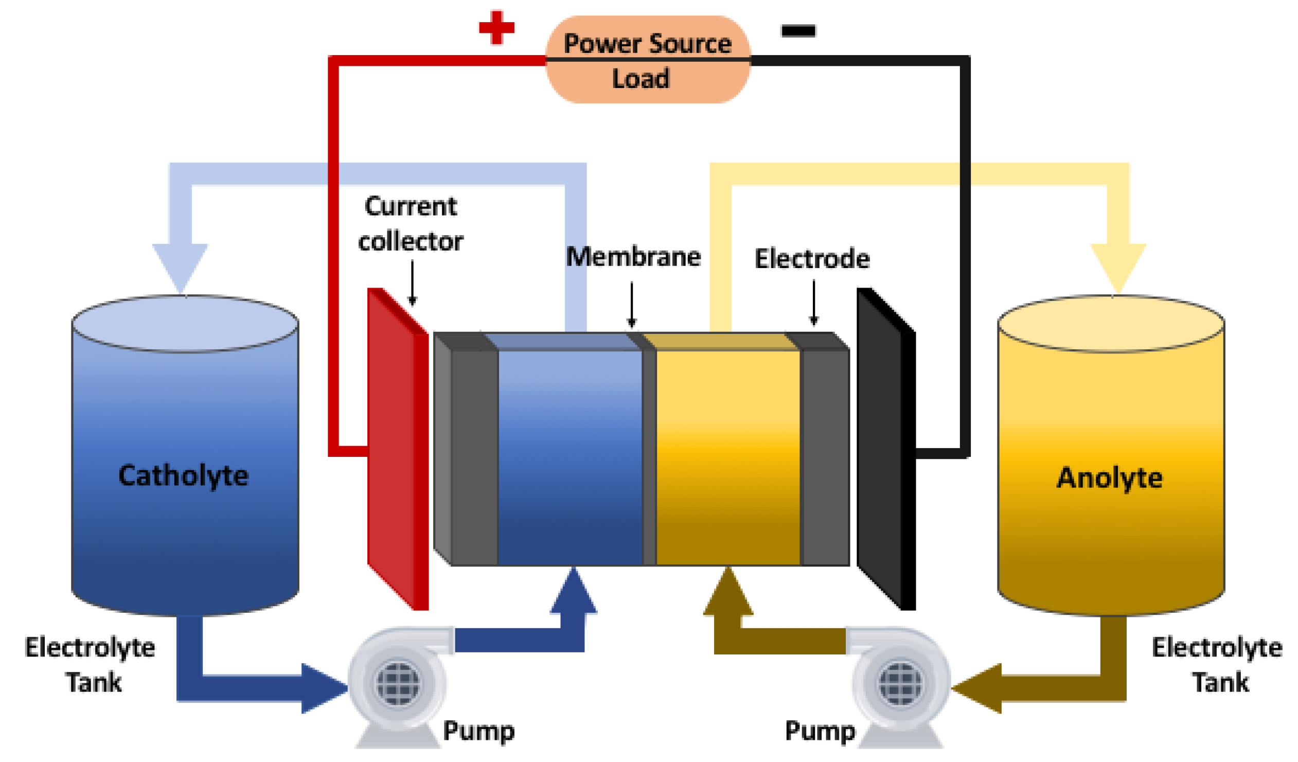
2.1. Operation of a VRFB

Figure 1 shows the conventional scheme of a RFB; it is composed by two tanks containing the electrolytes dissolved in solutions. These electrolytes are pumped by two coordinated pumps through a cell stack. It is in this cell where the oxidation reduction reaction (REDOX) and the electric current is absorbed or generated. The electrolytes return to the tanks with a different concentration of species from the initial one. The species concentration in the tanks is directly related with the stored energy, i.e., the state of charge (SOC); while, the species concentration in the cell is directly related with the output voltage.

In a VRFB, the electrolytes contain salts of vanadium dissolved in solutions of sulphuric acid. In this case, all of the species are vanadium in different oxidation states (+II, +III, +IV, +V). The anolyte is composed by $V^{2+}$ and $V^{3+}$ vanadium species, while the catholyte is composed by $V^{4+}$ and $V^{5+}$. It is important to notice that the vanadium species $V^{4+}$ and $V^{5+}$ exist as oxides, which are $V{O}^{2+}$ and $V{O}_2^{+}$, respectively.

During the charging process, $V^{4+}$ oxidizes to $V^{5+}$, releasing an electron, which is transferred from the cathode to the anode, reducing $V^{3+}$ to $V^{2+}$. The total reaction can be written as

$$\begin{array}{ccc}\hfill V^{2+}& \to & V^{3+}+e^{-}\hfill \\ \hfill V{O}_2^{+}+2H^{+}+e^{-}& \to & V{O}^{2+}+H_{2}O\hfill \end{array}$$

(1)

The process occurs in the reverse direction during the discharge. Subsequently, it is possible to conclude that, depending on the amount of electrons that appear on the cell in a discharging or charging process, the concentration of each specie will vary according to the reaction that is presented in (1).

The voltage in the cell can be computed while using the Nerst equation. This allows to know which is the electrode potential that appears in the extremes of a cell while taking the different concentrations of vanadium species contained on it into account. The electrode potential E has the following expression [31]:

$$E=E^{\theta }+\frac{RT}{F}ln\left[{\left(\frac{c_5^{cell}}{c_4^{cell}}\right)}_{catholyte}{\left(\frac{c_2^{cell}}{c_3^{cell}}\right)}_{anolyte}\right],$$

(2)

where R and F are, respectively, the gas and Faraday constant, T is the temperature, $E^{\theta }$ is the standard electrode potential, and $c_i^{cell}$ is the concentration of vanadium specie i in the cell.

Experimentally, it has been found that the maximum value of the cell voltage during the charging process varies between 1.6 and 1.7 V, and then drops to 1.1 V during discharging [31,32]. As this value is low, in order to increase the voltage, different cells are connected in series, defining what is usually known as a stack.

The RFB state of charge (SOC), which corresponds the amount of energy that is stored in the tanks, can be computed as a function of the vanadium species contained in the tank as:

$$SOC=\left(\frac{c_2^{tank}}{c_2^{tank}+c_3^{tank}}\right)=\left(\frac{c_5^{tank}}{c_4^{tank}+c_5^{tank}}\right)$$

(3)

where $c_i^{tank}$ is the concentration of vanadium specie i in the tank. The index $i=2$ corresponds to $V^{2+}$, $i=3$ to $V^{3+}$, $i=4$ to $V^{4+}$ (which exists as $V{O}^{2+}$) and $i=5$ (which exists as $V{O}_2^{+}$). This same convention is used in the cell concentration.

2.2. VRFB Electrochemical Model

One of the most popular models for describing the electrochemical behaviour was introduced by Maria Skyllas-Kazacos [18]. It allows for describing the evolution of the vanadium species concentrations, both in the tanks and the cells and it has been experimentally validated with excellent results [18,25].

The equation describing the evolution of the vanadium species concentrations in the cell is given by:

$$\frac{V_{cell}}{2}{\dot{\mathbf{x}}}^{cell}=\left({\mathbf{x}}^{tank}-{\mathbf{x}}^{cell}\right)q^{cell}+\frac{1}{zF}\left(\begin{array}{c}1\\ -1\\ -1\\ 1\end{array}\right)i^{cell}+\frac{S}{d}\left(\begin{array}{cccc}-k_2& 0& -k_4& -2·k_5\\ 0& -k_3& 2·k_4& 3·k_5\\ 3·k_2& 2·k_3& -·k_4& 0\\ -2·k_2& -k_3& 0& -k_5\end{array}\right){\mathbf{x}}^{cell},$$

(4)

where ${\mathbf{x}}^{cell}={\left[c_2^{cell},c_3^{cell},c_4^{cell},c_5^{cell}\right]}^T$, ${\mathbf{x}}^{tank}={\left[c_2^{tank},c_3^{tank},c_4^{tank},c_5^{tank}\right]}^T$, $V_{cell}$ is the volume of the cell, $q^{cell}$ is the electrolyte flow rate, $i^{cell}$ is the current in the cell (positive and negative currents define the charging and discharging process, respectively), z is the number of electrons that are involved in the reaction ($z=1$), S is the surface and d the thickness of the membrane, and finally, $k_i$ is the diffusion coefficient for vanadium specie i. Equation (4) can be rewritten in a more compact form as:

$${\dot{\mathbf{x}}}^{cell}={\mathbf{f}}^{cell}\left({\mathbf{x}}^{cell},{\mathbf{x}}^{tank},i^{cell},q^{cell}\right).$$

(5)

The equation describing the tank concentration considering the number of cells that compose the stack is:

$$V_{tank}{\dot{\mathbf{x}}}^{tank}=N\left({\mathbf{x}}^{cell}-{\mathbf{x}}^{tank}\right)q^{cell},$$

(6)

where $V_{tank}$ is the volume of each electrolyte tank and N is the number of cells that compose the stack.

Equations (5) and (6) define a dynamical system that describes the electrochemical behaviour in the RFB. In this model, ${\mathbf{x}}^{cell}$ and ${\mathbf{x}}^{tank}$ are the state variables and and $q^{cell}$ and $i^{cell}$ are two exogenous variables. From a control perspective, $q^{cell}$ is usually assumed as the control action, while $i^{cell}$ is considered to be a measurable disturbance.

In this work, a 3 kW and 15 kWh VRFB system has been considered with a total vanadium concentration of 2 M for each couple of species. The other parameters that are needed to obtain the model are summarized in

Table 1. Parameters and constants for Nerst Equation.

Parameter	Meaning	Unit—Value
$c_i^{cell}$	Concentration of specie i inside the cell	$\mathrm{mol}·{\mathrm{m}}^{-3}$
E	Electrode potential	V
$E^{\theta }$	Standard potential	1.259 V
T	Temperature of the cell	K
F	Faraday’s constant	96,485 $\mathrm{C}·{\mathrm{mol}}^{-1}$
R	Gas constant	8.314 $\mathrm{J}·{\mathrm{K}}^{-1}·{\mathrm{mol}}^{-1}$

and

Table 2. Parameters of the electrochemical model [18].

Parameter	Meaning	Unit—Value
$V_{cell}$	Volume of the cell	$9.5·{10}^{-4}$${\mathrm{m}}^3$
$V_{tank}$	Volume of each tank	$0.4$${\mathrm{m}}^3$
Q	Flow rate	${\mathrm{m}}^3·{\mathrm{s}}^{-1}$
I	Current	$\mathrm{A}$
S	Surface area of the electrode	0.15 ${\mathrm{m}}^2$
d	Membrane thickness	1.27·10${}^{-4}$ $\mathrm{m}$
$k_2$	Diffusion coefficient of $V^{2+}$	$8.768·{10}^{-12}$$\mathrm{m}·{\mathrm{s}}^{-1}$
$k_3$	Diffusion coefficient of $V^{3+}$	$3.221·{10}^{-12}$$\mathrm{m}·{\mathrm{s}}^{-1}$
$k_4$	Diffusion coefficient of $V^{4+}$	$6.825·{10}^{-12}$$\mathrm{m}·{\mathrm{s}}^{-1}$
$k_5$	Diffusion coefficient of $V^{5+}$	$5.896·{10}^{-12}$$\mathrm{m}·{\mathrm{s}}^{-1}$
N	Number of cells of the stack	19

.

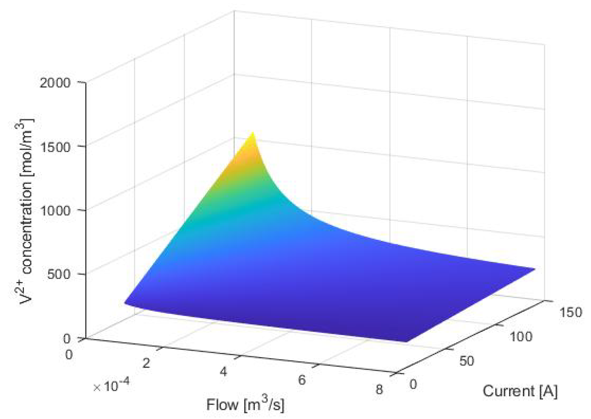
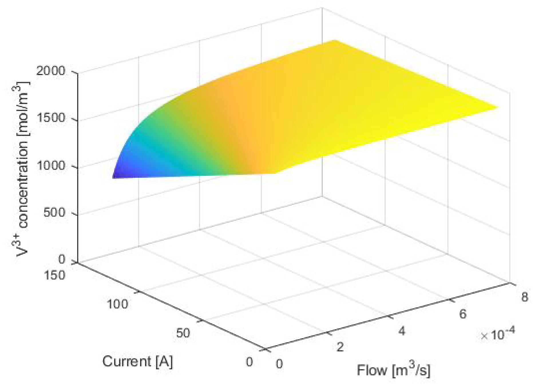
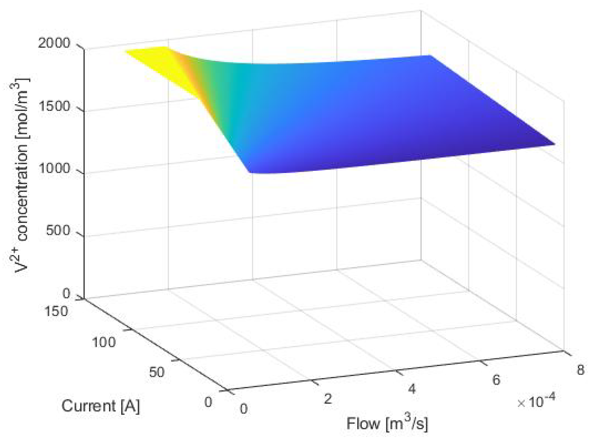
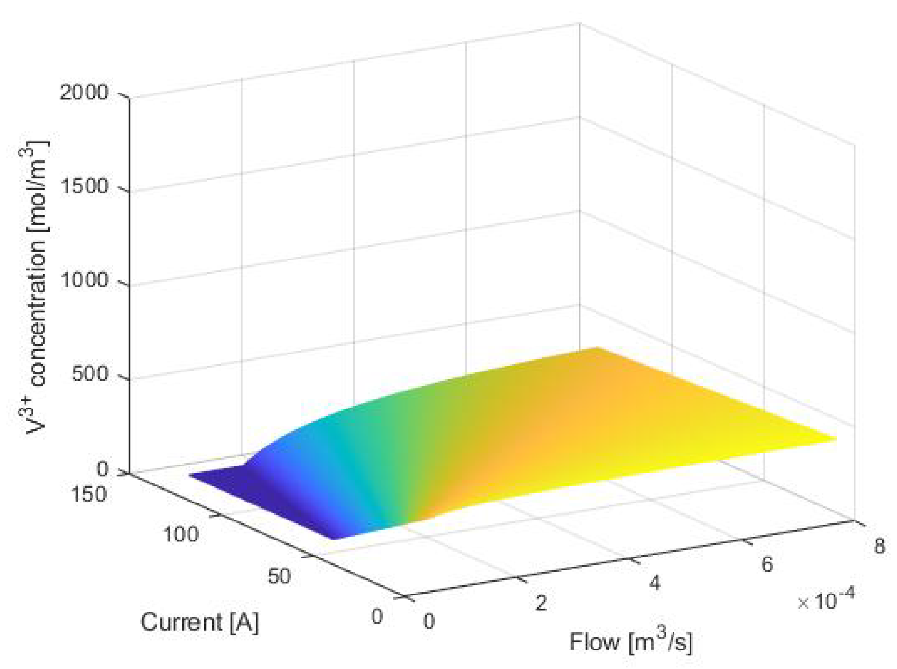
3. Equilibrium Points Analysis

Equilibrium points play a very important role in dynamical systems [33,34]. These points correspond to the configurations (values of the state variables) where the dynamic system can remain stationary, due to this they are also called operation points. The equilibrium points are the solutions that make the derivatives of the differential equations of a system equal to zero.

To compute the equilibrium points for the dynamic system defined by (5) and (6), it is necessary to force ${\dot{\mathbf{x}}}^{cell}=0$ and ${\dot{\mathbf{x}}}^{tank}=0$ and isolate the value of ${\mathbf{x}}^{cell}$ and ${\mathbf{x}}^{tank}$. Because (5) and (6) depend on $i^{cell}$ and $q^{cell}$, there is no solution, but $i^{cell}=0$, $q^{cell}=0$, ${\mathbf{x}}^{cell}=0$, and ${\mathbf{x}}^{tank}=0$, which is clearly not of interest.

In RFB, the volume of the tanks, $V_{tank}$, is much bigger than the volume of the cell, $V_{cell}$, and, consequently, the variation of ${\mathbf{x}}^{tank}$ is tiny in comparison to the variation of ${\mathbf{x}}^{cell}$. Therefore, a natural assumption is to assume that ${\dot{\mathbf{x}}}^{tank}\approx 0$, which implies that ${\mathbf{x}}^{tank}$ is constant, i.e., SOC is constant. Under this assumption, the equilibrium points of (5) can be found. These equilibrium points will depend on the value of ${\mathbf{x}}^{tank}$, i.e., the SOC, $i^{cell}$ and $q^{cell}$.

From the analysis of these points, it is possible to determine which is the optimal $q^{cell}$, once the SOC and $i^{cell}$ have been fixed. Figure 2 and Figure 3 show the values of $V^{2+}$ and $V^{3+}$ in the cell for a 10% of SOC, a different values of $i^{cell}$, from 10 to 140 A, and $q^{cell}$ from 75 mL/s to 800 mL/s [26,35,36]. Figure 2 and Figure 3 are representative of a charging procedure.

Becasue the total vanadium concentration is 2000 $\mathrm{mol}/{\mathrm{m}}^3$, the vanadium concentration in the cell is limited to this value. For a 10% of SOC, the concentration in the anolyte tank corresponds to 200 $\mathrm{mol}/{\mathrm{m}}^3$ for $V^{2+}$ and 1800 $\mathrm{mol}/{\mathrm{m}}^3$ for $V^{3+}$.

Looking at Figure 2 and Figure 3, it can be observed that the surface stay as an horizontal plane at the majority of current and flow points. This behaviour is observed, especially at flow rates that are greater than $0.2$ $\mathrm{L}/\mathrm{s}$. This means that concentration in the cell is almost the same in the tank for high flow rates. In the case of $V^{2+}$ is 200 $\mathrm{mol}/{\mathrm{m}}^3$, and for $V^{3+}$ is 1800 $\mathrm{mol}/{\mathrm{m}}^3$.

However, at a low enough flow rate, the surface is heading upwards for the more negative specie, which is $V^{2+}$, and downwards for the more positively charged $V^{3+}$. This behaviour can be better appreciated as the current increases, reaching the corresponding maximum or minimum at the lowest flow with the highest current.

When the RFB is charging, introducing a certain positive current, the more positively charged ion, which is $V^{3+}$, is reduced by the corresponding electrons of the current, which convert them to their counterpart, the more negatively charged ions $V^{2+}$.

When the flow is lower, more time is necessary in order to take the ions in the cell to get out of it. In terms of current, as it increases, a faster reduction happens. When both circumstances happen, the reduced ions begin to build up on the cell itself, which is why that upwards tilting begins to happen with vanadium specie $V^{2+}$. In counterpart, the vanadium concentration of ions $V^{3+}$ decreases with a behavior that is contrary to that of $V^{2+}$.

Figure 4 and Figure 5 show the values of $V^{2+}$ and $V^{3+}$ in the cell for an 80% of SOC, which implies having 1600 $\mathrm{mol}/{\mathrm{m}}^3$ of $V^{2+}$ specie, and 400 $\mathrm{mol}/{\mathrm{m}}^3$ $V^{2+}$ inside the tank. In this new situation, the surface gets to his maximum possible concentration for $V^{2+}$, which is 2000 $\mathrm{mol}/{\mathrm{m}}^3$, and the minimum, which is 0 $\mathrm{mol}/{\mathrm{m}}^3$ for $V^{3+}$ specie. This maximum value can be observed in Figure 4, which is represented in yellow. On the other case, the minimum concentration of 0 mol/m${}^3$ is observed in dark blue in Figure 5.

With these studies, it is possible to characterize the stationary behavior of the different concentrations and, therefore, of the voltage in the cell. The behavior has been analyzed for a loading and unloading scenario, but it is possible to do it for other SOC values. The behavior evolves smoothly between the two examples presented.

4. Controller Design

4.1. Introduction

Differently from other types of batteries, like Li-on, RFB are active elements, i.e., it is necessary to feed the cell with reactants. Because of this, it is necessary to design a control system that guarantees the correct closed-loop behavior. The RFB has two inputs, the current, $i^{cell}$, and the flow rate, $q^{cell}$, as discussed in Section 2. From a control point of view, $i^{cell}$ is treated as measurable disturbance, while $q^{cell}$ is used as control action. A very relevant measurable variable is the output voltage, E. The voltage combined with the current determine the input/output power.

In this section, a voltage controller will be designed. The methodology that is used to design the controller is based on the $H_{\infty }$ control theory, which allows for synthesizing controllers that guarantee performance specifications and, at the same time, achieve the stabilization of the system.

Linear $H_{\infty }$ methods [37] are used to shape the frequency response of the most relevant closed-loop transfer functions in a control system. This shaping is formulated as an optimization problem in terms of the infinity norm: $\left|\right|·{\left|\right|}_{\infty }$. The procedure to design a controller is based on two steps; in the first one, the specifications are defined through the use of weighting functions that can be understood as bounds over the frequency response. Once the specifications are made, the optimal controller is obtained, i.e., the controller is the one that better fulfils the specifications in terms of the $\left|\right|·{\left|\right|}_{\infty }$. One of the main advantages of the $H_{\infty }$ design method is that it permits dealing with model and parametric uncertainties. In this way, we can design controllers that preserve closed-loop stability and desired performance in spite of plant uncertainties. These characteristics can be applied in order to design the control system of the redox battery. In this case, with the distinct equilibrium points of the system, we can create a structure for the plant composed of a nominal model of the battery that is associated to a norm-bounded uncertainty. On this base, the $H_{\infty }$ design is used to accomplish closed-loop stability and performance in a wide range of operating conditions.

4.2. Model Simplification

Before designing the controller, the plant model (5) will be simplified. To do so, the following assumptions can be made:

• Vanadium concentrations are the same on both sides of the half cell. Therefore, it is possible to have the following correspondence:

  $$c_2^{cell}=c_5^{cell}{c}_3^{cell}=c_4^{cell}$$
• The tanks concentration can be expressed in terms of SOC and total vanadium concentration $c_v$:

  $$c_2^{tank}=c_{v}SOC{c}_3^{tank}=c_v·(1-SOC)$$

Taking into account these equalities, it is possible to express the electrochemical model, reducing Equations (4) and (2) to:

$$\begin{array}{ccc}\hfill V_{cell}\frac{d}{dt}\left[\begin{array}{c}{c}_2^{cell}\\ c_3^{cell}\end{array}\right]& =& \left[\begin{array}{c}{c}_v·SOC-c_2^{cell}\\ c_v·(1-SOC)-c_3^{cell}\end{array}\right]q^{cell}+\left(\begin{array}{c}\frac{1}{F}\\ -\frac{1}{F}\end{array}\right)i^{cell}+\frac{S}{d}\left(\begin{array}{cc}-k_2-2k_5& -k_4\\ 3k_5& -k_3+2k_4\end{array}\right)\left[\begin{array}{c}{c}_2^{cell}\\ c_3^{cell}\end{array}\right]\hfill \end{array}$$

(7)

$$\begin{array}{ccc}\hfill E& =& E^{\theta }+\frac{2NRT}{F}ln\left(\frac{c_2^{cell}}{c_3^{cell}}\right),\hfill \end{array}$$

(8)

respectively.

4.3. System Linearization

The system that is defined by (7) and (8) can be easily transformed in the standard nonlinear state space form:

$$\begin{array}{ccc}\hfill \dot{\mathit{x}}& =& \mathit{f}(\mathit{x},\mathit{u})\hfill \\ \hfill y& =& h(\mathit{x},\mathit{u})\hfill \end{array}$$

with $y=E$, $\mathbf{x}={\left[c_2^{cell},c_3^{cell}\right]}^T$ and $\mathit{u}={\left[i^{cell},q^{cell}\right]}^T$. This model can be linearized around its equilibrium points ($\overline{\mathit{x}},\overline{u}$), using the Taylor series, as follows:

$$\mathit{f}(\mathit{x},u)=\mathit{f}(\overline{\mathit{x}},\overline{u})+{\left.\frac{\partial \mathit{f}}{\partial \mathit{x}}\right|}_{\overline{\mathit{x}},\overline{u}}\mathsf{\Delta }\mathit{x}+{\left.\frac{\partial \mathit{f}}{\partial u}\right|}_{\overline{\mathit{x}},\overline{u}}\mathsf{\Delta }u+h.o.t(\mathsf{\Delta }\mathit{x},\mathsf{\Delta }u)$$

$$h(\mathit{x},u)=h(\overline{\mathit{x}},\overline{u})+{\left.\frac{\partial h}{\partial \mathit{x}}\right|}_{\overline{\mathit{x}},\overline{u}}\mathsf{\Delta }\mathit{x}+{\left.\frac{\partial h}{\partial u}\right|}_{\overline{\mathit{x}},\overline{u}}\mathsf{\Delta }u+h.o.t(\mathsf{\Delta }\mathit{x},\mathsf{\Delta }u)$$

where $h.o.t$ denotes high order terms, which will be very close to zero if states ($\mathit{x},u$) are sufficiently close to its equilibrium points ($\overline{\mathit{x}},\overline{u}$).

It is possible to rewrite the linearized system in the state space form, as follows:

$$\begin{array}{ccc}\hfill \dot{\mathsf{\Delta }\mathit{x}}& =& \mathit{A}\mathsf{\Delta }\mathit{x}+\mathit{b}\mathsf{\Delta }u\hfill \\ \hfill \mathsf{\Delta }y& =& \mathit{c}\mathsf{\Delta }\mathit{x}+d\mathsf{\Delta }u\hfill \end{array}$$

where $\mathsf{\Delta }\mathit{x}=\mathbf{x}-\overline{\mathit{x}}$, $\mathsf{\Delta }u=u-\overline{u}$, and $\mathsf{\Delta }y=y-\overline{y}$, and $\mathit{A},\mathit{b},\mathit{c},d$ are the following jacobian matrices:

$$\mathit{A}={\left.\frac{\partial \mathit{f}}{\partial \mathit{x}}\right|}_{\overline{\mathit{x}},\overline{\mathit{u}}}\mathit{b}={\left.\frac{\partial \mathit{f}}{\partial u}\right|}_{\overline{\mathit{x}},\overline{\mathit{u}}}\mathit{c}={\left.\frac{\partial h}{\partial x}\right|}_{\overline{\mathit{x}},\overline{\mathit{u}}}d={\left.\frac{\partial h}{\partial u}\right|}_{\overline{\mathit{x}},\overline{\mathit{u}}}$$

For the system that is defined by (7) and (8), the Jacobian matrices become:

$$\begin{array}{ccc}\mathit{A}\hfill & =& \frac{1}{V_{cell}}\left[\begin{array}{cc}\frac{S}{d}(-k_2-2k_5)-{\overline{q}}^{cell}& \frac{S}{d}(-k_4)\\ \frac{S}{d}\left(3k_5\right)& \frac{S}{d}(k_4-k_3)-{\overline{q}}^{cell}\end{array}\right]\hfill \end{array}$$

(9)

$$\begin{array}{ccc}\mathit{b}\hfill & =& \frac{1}{V_{cell}}\left[\begin{array}{c}{c}_{v}SOC-{\overline{c}}_2^{cell}\\ c_v(1-SOC)-{\overline{c}}_3^{cell}\end{array}\right]\hfill \end{array}$$

(10)

$$\begin{array}{ccc}\mathit{c}\hfill & =& \left[\begin{array}{cc}\frac{2NRT}{F}·\frac{1}{{\overline{c}}_2^{cell}}& -\frac{2NRT}{F}·\frac{1}{{\overline{c}}_3^{cell}}\end{array}\right]\hfill \end{array}$$

(11)

$$\begin{array}{ccc}d\hfill & =& 0\hfill \end{array}$$

(12)

The system defined by $(\mathit{A},\mathit{b},\mathit{c},d)$ allows for analyzing the nonlinear system behavior around the equilibrium point.

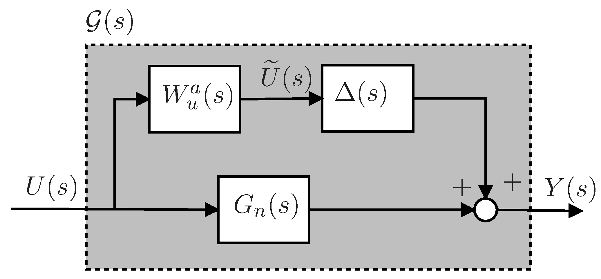
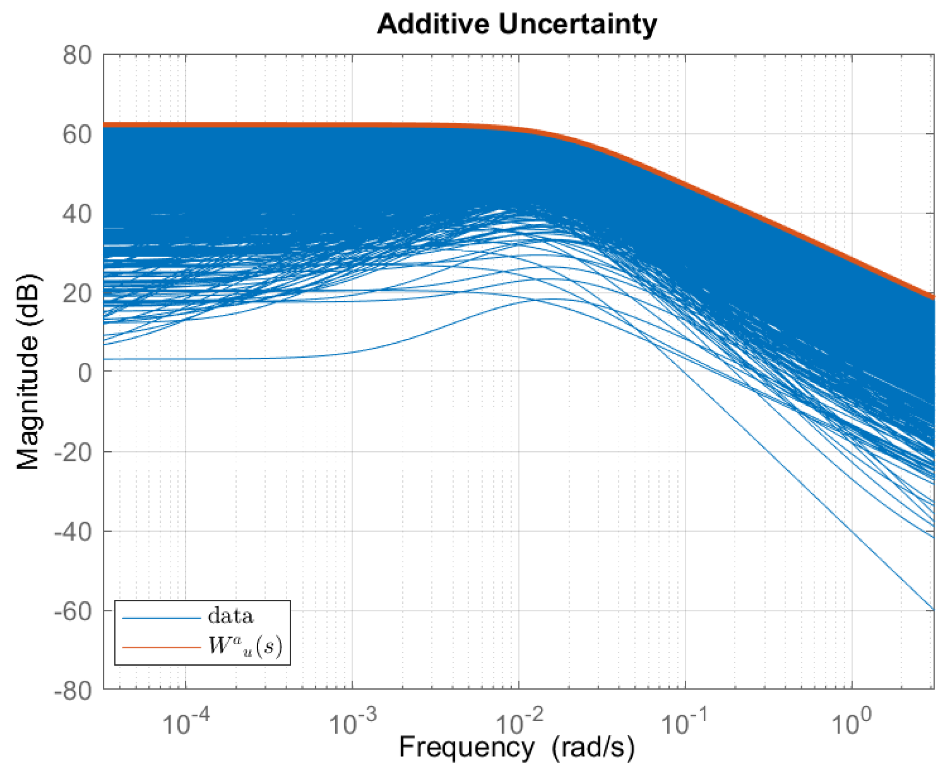
4.4. Uncertainty Modeling

The values $(\mathit{A},\mathit{b},\mathit{c},d)$ defined by (9)–(12) depend on the value of different parameters, the value of the SOC, and the concrete equilibrium point. Figure 6 shows the frequency response of different linear plants obtained sweeping the value of SOC between 10% to 90%, which corresponds to almost a full charged or discharged VRFB and sweeping the current value from 15 to 120 A (for both charging and discharging modes). Similarly, Figure 7 shows the step response of these linear models. As it can be seen, there is an important variability in both gain and time constant. It is important to take this variability in the controller design into account. A model with uncertainty will be developed in order to design a controller that can operate while taking into account all possible range of operation of SOC, current, and flow rate.

Figure 8 shows the block scheme of a plant with additive uncertainty, in this scheme $G_n\left(s\right)$ is the nominal plant, $W_u^a\left(s\right)$ is a weighting function that provides bounds on how the real plant might change from the nominal one, and $\mathsf{\Delta }\left(s\right)$ is an uncertainty function, such that $\parallel \mathsf{\Delta }\left(s\right)\parallel <1$.

The nominal plant has been selected while using the nominal parameters (Table 2), a value of SOC of 50%, and a current of 70 A. These parameters are averaged values and they offer an average behaviour in both frequency and step response. The selected nominal plant corresponds to a 2nd order transfer function:

$$G_n\left(s\right)=\frac{-24.36s-0.3966}{s^2+0.03256s+0.0002651}$$

Once the nominal plant has been defined, the value of $W_u^a\left(s\right)$ will be obtained. Hence, the following procedure will be followed:

• Select a relevant number of plants which represent all possible values of (9)–(12). In this work, 2000 plants have been selected.
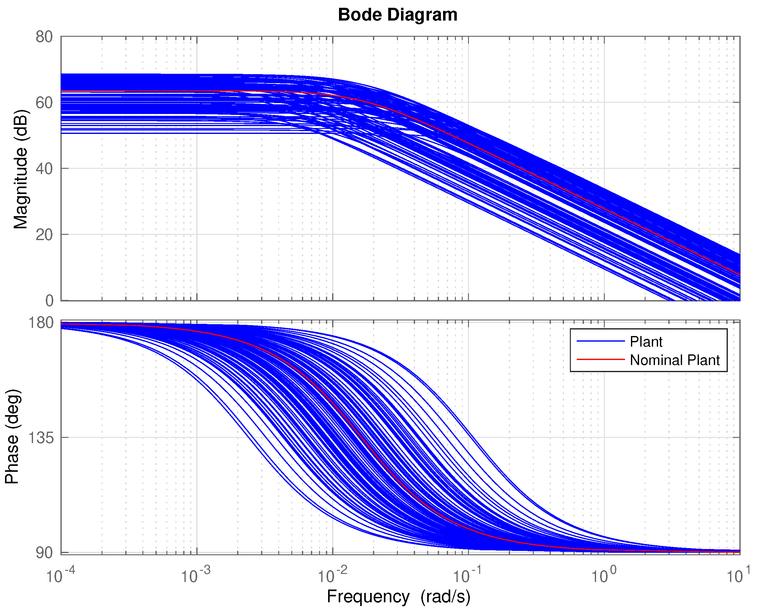
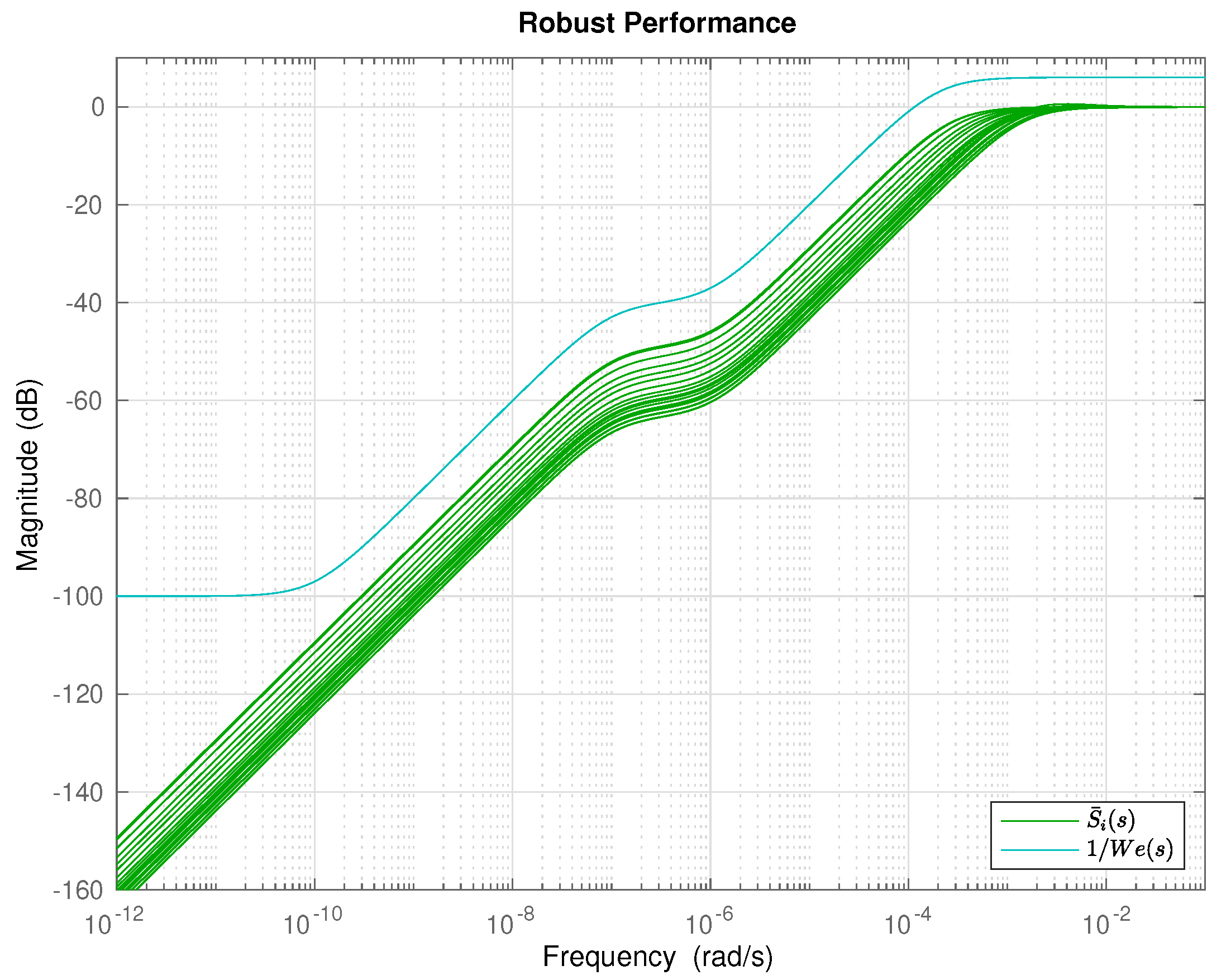
• Determine a frequency range where to model the uncertainty. In our case the, range $[{10}^{-4.5},{10}^{0.5}]$ $\mathrm{rad}/\mathrm{s}$ has been selected. As can be seen in Figure 6, out of this frequency range there is almost no variability in the response. 500 points logarithmically distributed have defined in this range.
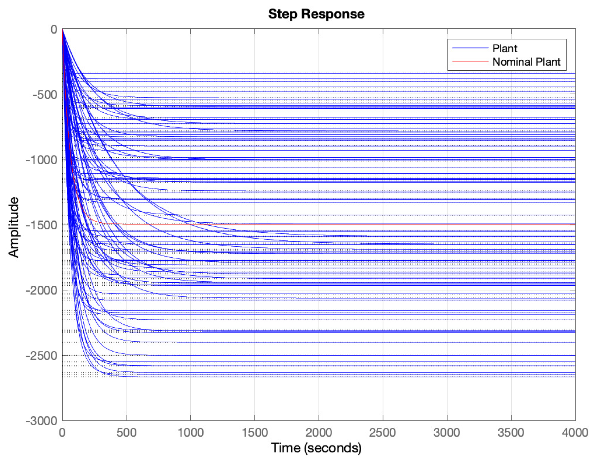
• Sample the set of plants, obtained in step 1 and the range of frequencies selected in step 2.
• Compute the error (distance) between each point with respect the nominal plant.
• Obtain stable and minimum phase rational function of polynomials that bounds all of the points obtained in step 4. The rational function order must be selected making a trade-off between the order of the function and the goodness of the fit.

Figure 9 shows the error obtained in step 4 and the fitting function. The corresponding weighting $W_u^a\left(s\right)$ is then a second order transfer function:

$$W_u^a\left(s\right)=\frac{2.0436(s+12.62)(s+0.2006)}{(s+0.2318)(s+0.01745)}$$

An almost perfect fitting is obtained, as it can be seen. This weighting function is calculated while using the cover function from the MATLAB Robust Control Toolbox [38].

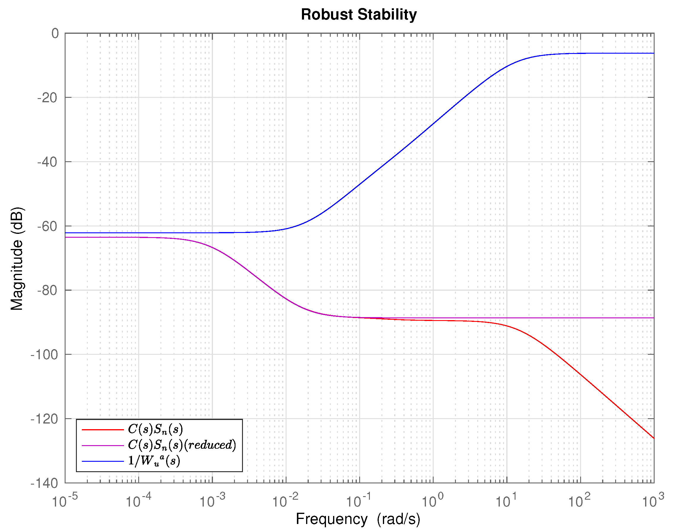
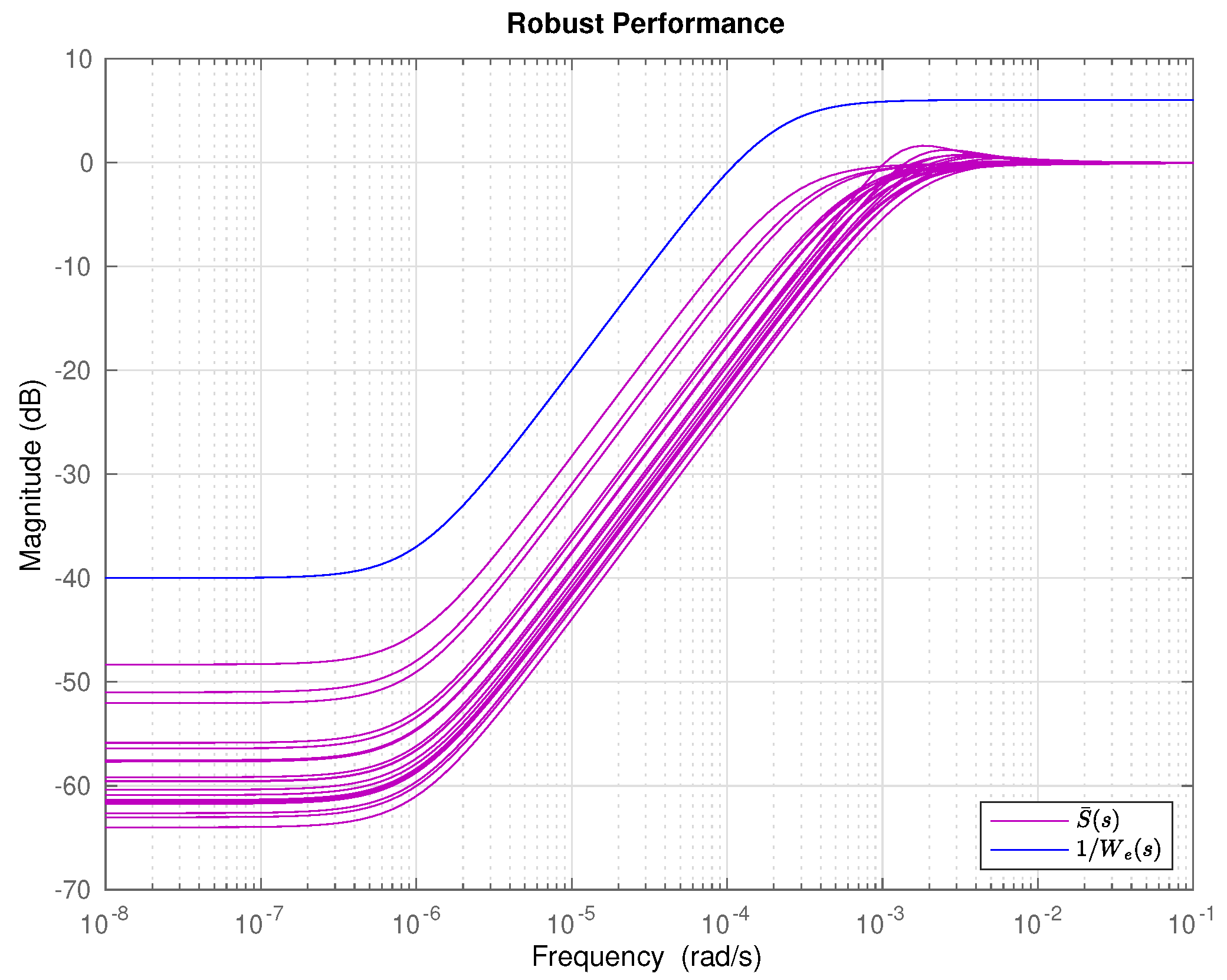
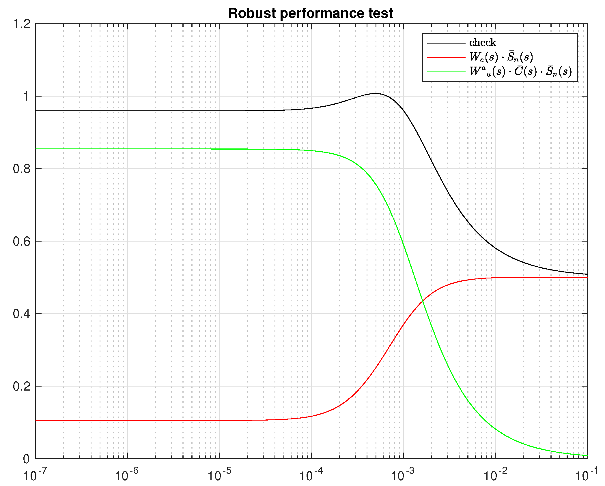
4.5. Controller Design

Figure 10 shows the proposed feedback configuration for the control of the redox battery. The configuration is composed of the nominal plant $G_n\left(s\right)$, the controller $C\left(s\right)$, the uncertainty term $\mathsf{\Delta }\left(s\right)$, and the weighting functions $W_u^a\left(s\right)$ to shape the plant uncertainty. Finally, a new term $W_e\left(s\right)$ is added in order to define the system performance specification. With this configuration, it will be possible to determine the conditions for performance and stability.

Firstly, the performance specification will be defined. In this way, the nominal sensitivity function will be used to specify the performance; this transfer function relates the error and reference signals:

$$S_n\left(s\right)=\frac{E\left(s\right)}{R\left(s\right)}=\frac{1}{1+C\left(s\right)G_n\left(s\right)}.$$

The sensitivity function also relates the output disturbance with the error. To define bounds on the sensitivity function, the following weigthing function is usually used [37]:

$$W_e\left(s\right)=\frac{1}{M_s}\left[\frac{s+M_s{w}_b}{s+ϵw_b}\right]$$

(13)

where $M_s$ takes a value between 1 and 2 and it is directly related to the nominal robustness, i.e., gain and phase margins, $ϵ$ is a bound on the steady-state error, and $w_b$ is used to fix the closed-loop bandwidth, which is related to the system settling time.

The steady-state error tolerance has been selected to be less than 1% to guarantee a precise tracking of the reference. A value of $M_s$ equal to 2 has been selected; this value guarantees a distance of 0.5 to the critical point (−1,0), a gain margin that is greater than 2 and phase margin greater of 30${}^{\circ }$. In terms of bandwidth, it has been selected a frequency of ${10}^{-4}$ $\mathrm{rad}/\mathrm{s}$. Figure 11 shows the frequency response of $W_e^{-1}\left(s\right)$, in blue, which defines the desired bounds over the nominal sensitivity function, $S_n\left(s\right)$. Therefore, to accomplish the performance specifications, we have:

$$|S_n\left(j\omega \right)|<\frac{1}{|W_e\left(j\omega \right)|},\forall \omega$$

which is equivalent to:

$${\parallel W_e\left(s\right)S_n\left(s\right)\parallel }_{\infty }<1.$$

(14)

This equation corresponds to the Nominal Performance (NP) condition, which implies that the closed-loop system without uncertainty, i.e., $W_u^a\left(s\right)=0$, fulfils the specified performance.

Secondly, the design must guarantee closed-loop stability despite the plant uncertainty. This is known as Robust Stability Condition (RS). Based on the control system structure that is shown in Figure 10, the RS condition is [37]:

$${\parallel W_u^a\left(s\right)C\left(s\right)S_n\left(s\right)\parallel }_{\infty }<1.$$

(15)

An $H_{\infty }$ problem will be defined in order to design a controller that guarantees NP and RS conditions. Figure 12 shows the required augmented plant [37]. It can be observed the appearance of an augmented plant, called $P\left(s\right)$, with input vector ${\left[R\left(s\right)U\left(s\right)\right]}^T$ and output vector ${\left[\tilde{E}\left(s\right)\tilde{U}\left(s\right)E\left(s\right)\right]}^T$, and the controller $C\left(s\right)$ that adopts the conventional feedback path between $E\left(s\right)$ and $U\left(s\right)$.

In order to obtain a controller that guarantees (14) and (15)m the following Mixed sensitivity problem can be formulated:

$$\underset{C\left(s\right)}{\mathit{min}}{∥\begin{array}{c}{W}_e\left(s\right)S_n\left(s\right)\\ W_u^a\left(s\right)C\left(s\right)S_n\left(s\right)\end{array}∥}_{\infty }.$$

(16)

In case the obtained controller makes the $H_{\infty }$ norm less than one, then the NP and RS conditions will be guaranteed. From Figure 12 and Equation (16), we seek a stabilizing controller $C\left(s\right)$, with input $Y\left(s\right)$ and output $U\left(s\right)$, that minimizes the $H_{\infty }$ norm from $R\left(s\right)$ to ${\left[\tilde{E}\left(s\right)\tilde{U}\left(s\right)\right]}^T$.

With all previous definitions and configurations for performance and plant uncertainty, the optimization procedure yields a fifth order controller, $C\left(s\right)$. This order is exactly the same as that of the augmented plant. Note that, the augmented plant, $P\left(s\right)$ (see Figure 12), is composed by the nominal plant, $G_n\left(s\right)$, which is order 2, the sensitivity function weighting function, $W_e\left(s\right)$, which is of order 1 and the uncertainty weighting function, $W_u^a\left(s\right)$, which is order 2.

The resulting controller makes $∥\begin{array}{c}{W}_e\left(s\right)S_n\left(s\right)\\ W_u^a\left(s\right)C\left(s\right)S_n\left(s\right)\end{array}∥=0.86$, which is less than 1, so both the NP and RS are obtained. Figure 11 shows the frequency responses of the obtained nominal sensitivity function, $S_n\left(s\right)$, and the inverse of $W_e\left(s\right)$. The NP is fulfilled, as the frequency response of $S_n\left(s\right)$ is below the performance specifications. Figure 13 shows a graphical representation of the the RS condition. Because the curve for $C\left(s\right)S_n\left(s\right)$ is below the frequency response of $1/W_u^a\left(s\right)$, the robust stability condition is met.

The resulting order of the controllers designed using the $H_{\infty }$ method is usually high, which is a drawback for practical implementations. The order of the previous controller is five and it is desirable to obtain a lower order controller.

For that reason, a reduction of the order of the controller has been performed. The reduction is based on obtaining a balanced realization, which is a representation in the state space. The states are ordered by the so-called singular Hankel values, which give an idea of the observability and controllability of the different states by assigning them a certain value. The states that are below a certain tolerance of singular value are less significant to the system, having a negligible contribution to the I/O response. Eliminating these states, it is possible to reduce the order of the controller without altering their behaviour against the control of the system [37]. Using this approach, a reduced 2nd order controller, $\overline{C}\left(s\right)$, has been obtained. Figure 14 compares both the original and the reduced-order controller. As it can be seen, both controllers shows approximately the same frequency response. Only at high frequencies appears the difference. This is not a problem, since the controlled system works at low frequencies where it has been seen is the part where the uncertainty has more weight. Both NP and RS are preserved; consequently, the reduced order controller offers similar performance while facilitating the implementation and requiring less computational resources, as shown in Figure 11 and Figure 13.

Non-NP or RS guarantee that all possible plants fulfil the performance specifications; the proposed design procedure only guarantees performance over the nominal plant. Figure 15 shows the frequency response of the closed-loop sensitivity function of different plants, using the reduced order controller. As all drawn sensitivity frequency responses are below the specification curve, it can be assumed that, despite the uncertainty, all closed-loop systems fulfil the performance. This is called the Robust Performance (RP) condition. A more formal condition for RP, is [37]:

$$\parallel |W_e\left(s\right){\overline{S}}_n\left(s\right)|+|W_u^a\left(s\right)\overline{C}\left(s\right){\overline{S}}_n\left(s\right){|\parallel }_{\infty }<1$$

(17)

This condition can not be expressed as a regular $H_{\infty }$ problem, but it can be painted differentiating the NP and RS conditions, as it is shown in Figure 16. Figure 16 shows the formal robust performance analysis for the reduced order controller, $\overline{C}\left(s\right)$, as it can be seen, the black line corresponding to the bound defined in (17) is below 1 in almost all of the frequency range, but there is a small range of frequencies, around ${10}^{-3}$ rad/s, where the bound is over 1; this means that the RP condition is not fulfilled in this frequency range. For that reason, it can not be stated that the closed-loop system, as shown in Figure 10, fulfills RP, but, in practice, this controller can be considered to be good enough.

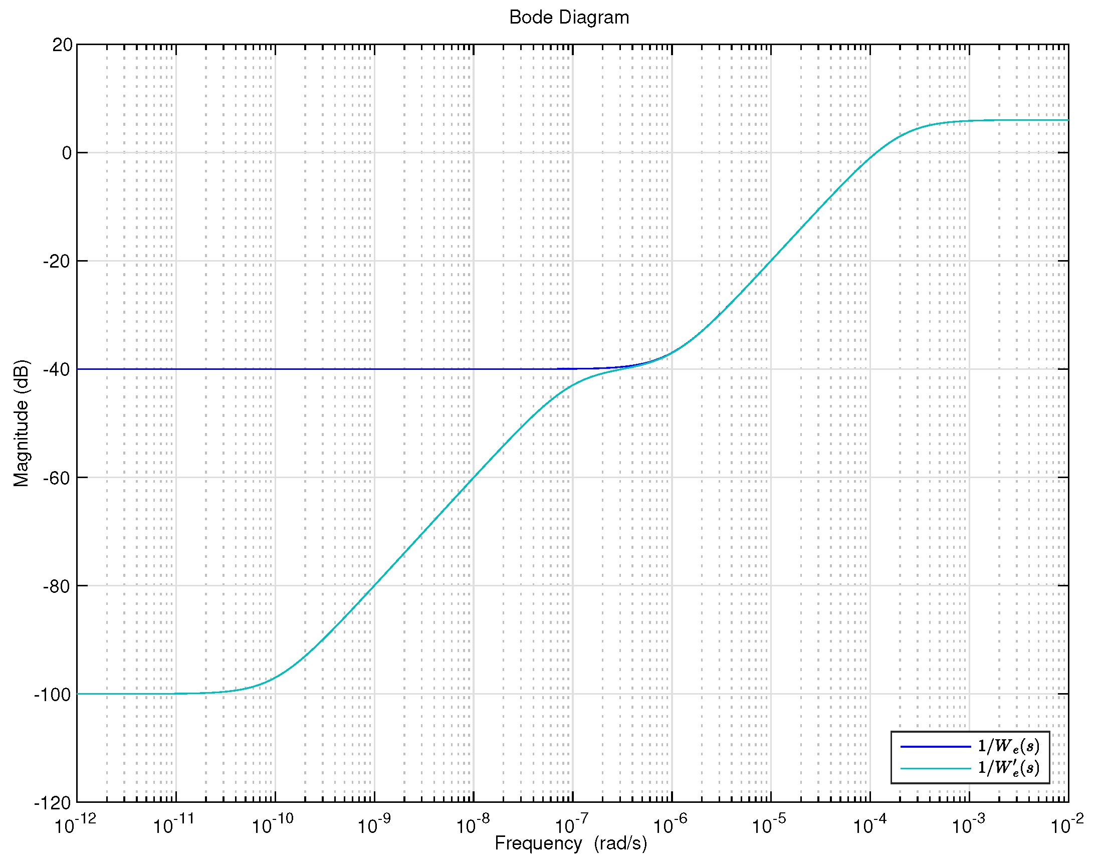
4.6. Integral Controller Design

It is well-known that integral action guarantees null steady-state error for constant or piecewise constant references. Unfortunately, $H_{\infty }$ control does not generate controllers with integral action in general. In order to eliminate the error against step-type reference changes, an integral part can be applied to the designed controller.

To force the appearance of an integral action in the controller, while preserving the nice properties of the $H_{\infty }$ framework, the weighting function for the nominal sensitivity function has been modified as:

$$W_e^{\prime }\left(s\right)=W_e\left(s\right)·\frac{s+K·{ϵ}^{\prime }}{s+{ϵ}^{\prime }}$$

(18)

where ${ϵ}^{\prime }$ must take the lowest possible value and K the highest one. Under these conditions, the dc gain of $W_e^{\prime }\left(s\right)$, will be $K/ϵ$. Consequently, an effect that is similar to placing a zero at $s=0$ in $W_e^{\prime }\left(s\right)$ will be achieved. This will force $|W_e^{\prime }\left(j\omega \right)|$ to be very high in the very low frequency range while preserving the frequency response of the original weighting function in the other frequencies.

Ideally, ${ϵ}^{\prime }$ should be practically zero, but computationally it is not possible to do so. In this work, after some numerical testing, $K={10}^3$ and ${ϵ}^{\prime }={10}^{-10}$ have been selected. Figure 17 shows a comparison between the bounds imposed by the original, $W_e\left(s\right)$, and the new, $W_e^{\prime }\left(s\right)$, weighting functions. As it can be seen, they are almost the same, but in the very low frequency range where $W_e^{\prime }\left(s\right)$ imposes harder constrains.

Once the weighting function has been redefined, the optimal controller is obtained again. Previous manipulations will force that the controller has a pole close to the origin. This pole is latter manually replaced by an integrator. This will generate an order 7 controller, $C_i\left(s\right)$. Note that, as the weighting function has increased its order, the controller also increased the order. This controller makes that $∥\begin{array}{c}{W}_e^{\prime }\left(s\right)S_{i,n}\left(s\right)\\ W_u^a\left(s\right)C_i\left(s\right)S_{i,n}\left(s\right)\end{array}∥=0.8605$ which is small than 1, this implies that this controller guarantees both NP and RS. As in the previous section, the order of this controller can be reduced up to order two, ${\overline{C}}_i\left(s\right)$. This controller can be rewritten as the Proportional, Integral, and Derivative (PID) one:

$$PID\left(s\right)={\overline{C}}_i\left(s\right)=k_p+\frac{k_i}{s}+\frac{k_{d}s}{\tau s+1}$$

(19)

with $k_p=-3.7053·{10}^{-5}$, $k_i=-6.7840·{10}^{-8}$, $k_d=0.0679$ and $\tau ={10}^6$. The PID Controller will be easier to implement on most platforms.

Figure 18 shows an informal proof of the RP condition. As it can be seen, all selected plants fulfil the specifications, which point up that the RP might be fulfilled. Figure 19 contains a formal analysis of the RP condition. The RP condition is not formally fulfilled, but it holds in almost all frequencies, which can be considered good enough from a practical point of view, as it can be observed. Finally, Figure 20 contains the step response of a number of plants, as it can be seen in all cases that a smooth response is obtained with null steady-state error.

4.7. Materials and Methods

The controller design procedure is one important result of this work. Figure 21 shows flowchart which summarizes the methodology introduced in previous subsections. Once the detailed non-linear model is defined, the design starts with the equilibrium point analysis. From this analysis, a set of representative operation points is selected, in each of these points the non-linear system is linearised; consequently, a set of linear models which cover the operation space is obtained. From this set of plants, a nominal plant, $G_n\left(s\right)$, with additive uncertainty, $W_u^a\left(s\right)$, is defined. At this point, the original non-linear system has been transformed into a linear system with uncertainty; consequently, linear techniques can be applied.

At this point, the closed-loop specifications are defined through a weighting function, $W_e\left(s\right)$, which define bounds over the closed-loop tracking error and the frequency response. Combining $G_n\left(s\right)$,$W_u^a\left(s\right)$ and $W_e\left(s\right)$, an augmented plant is built. Based on the augmented plant, the controller is synthesized using numerical methods. Once the controller is obtained, NP, RS and RP needs to be checked. If the specifications are meet, then a simulation against the original non-linear model is performed in order to guarantee the closed-loop behaviour, even for big movements (small movements around operation pints are constructively guaranteed). In case a wider operational range is needed, a larger set of linearised plant should be defined. The method should be iterated until all requirements are satisfactorily accomplished.

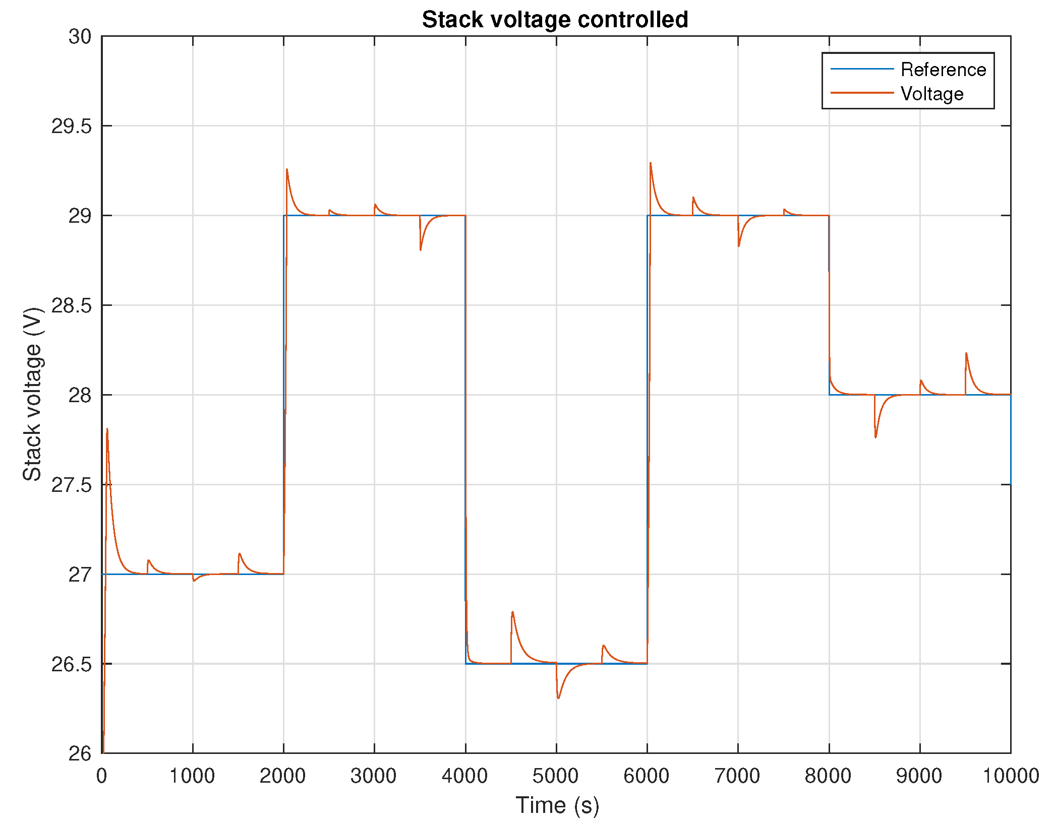
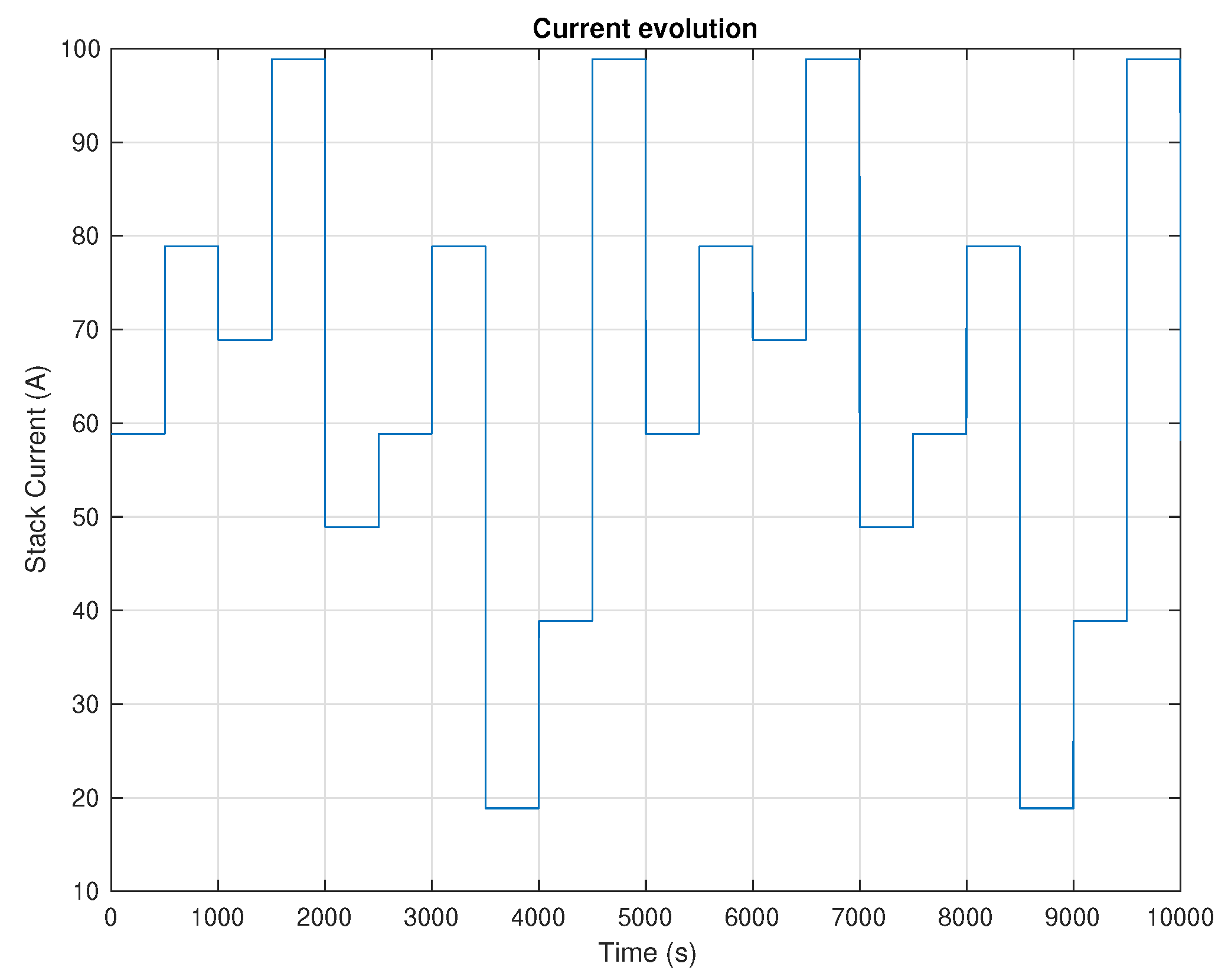
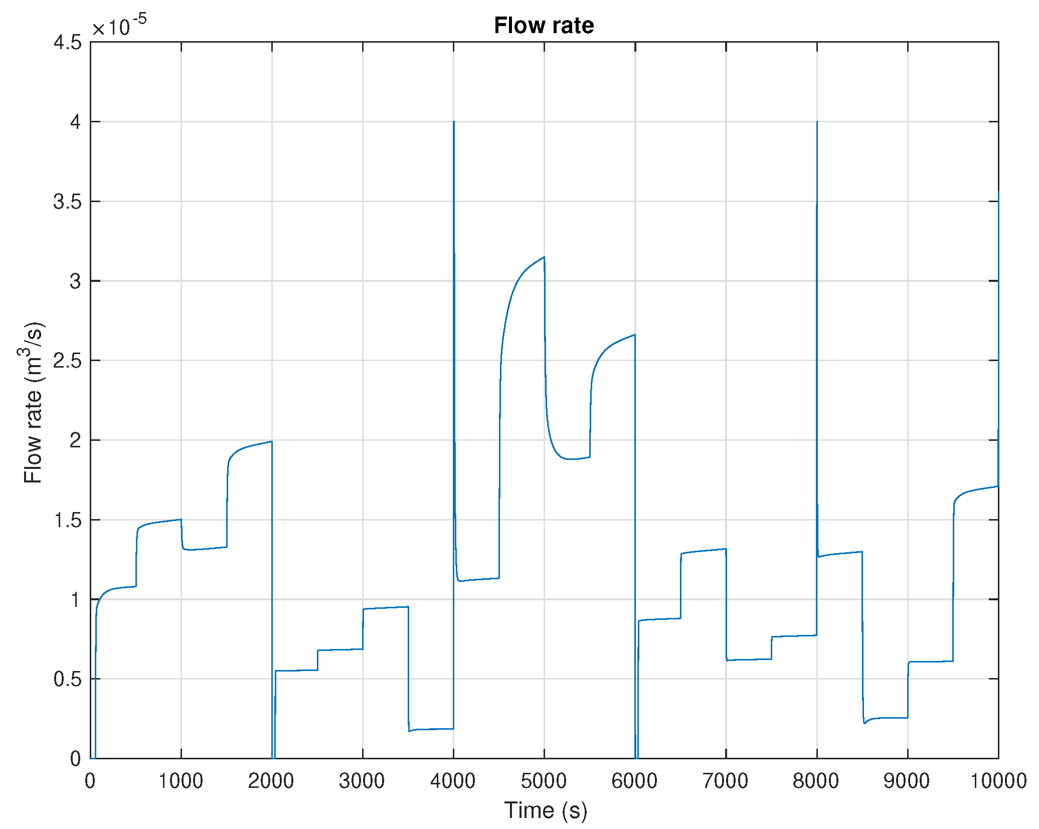
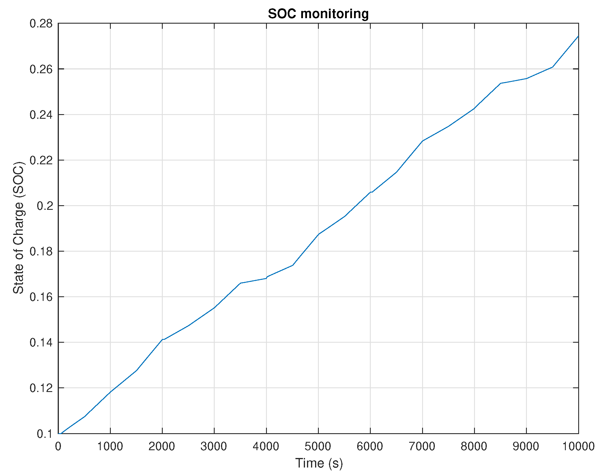
5. Results and Discussion

This section will show the results that were obtained using the controller proposed in Section 4.6. The controller will be validated using the complete non-linear model presented in Section 2. This model has been previously experimentally validated in the literature and it precisely reproduces the reality [18,25]. Figure 22 shows the simulation block scheme.

As the stack is composed by 19 cells, according to the Nerst equation, during the charging process, the voltage values might vary in a range between 26 to 31 V approximately (see Figure 23). Therefore, to analyse the behaviour of the controlled system, the voltage will be asked to follow a given voltage profile that is composed by different constant voltages. At the same time, it is important to study whether the controller is capable of operating under different current values. In this manner, uncertainty and disturbances are introduced in the system in terms of current. Hence, the current has been changed from 20 to 100 A in order to cover the full range. Figure 24 shows the profile of the current changes.

Figure 23 shows how the voltage tracks the voltage reference when using the low-order controller with integral part. As it can be seen, the stack voltage follows the reference with great precision. The steady-state error is 0 and the disturbances due to the current variations are successfully rejected. The transient response is satisfactory, even when voltage and current change simultaneously. This confirms that the robust designed controller behaves correctly against current and voltage variations.

Figure 25 shows the evolution of the flow rate generated by the proposed controller. As the flow rate is the control action, it is important to keep it bounded. With the defined operating conditions, it can be observed that the flow rate remains under $0.12$ mL/s. Larger peaks in flow rate can be seen when voltage and current change simultaneously; however, the maximum level of the control action ($4.5\times {10}^{-5}$ ${\mathrm{m}}^{-3}/\mathrm{s}$) is not reached.

It is important to note that neither current nor SOC are measured, only the voltage that is generated is used as the feedback signal. However, it is important to observe the evolution of the SOC. Figure 26 depicts the SOC against time for the given voltage and current profiles. Because current is always positive, the SOC is always increasing; this reflects the charging process of the VRFB.

Finally, it can be seen that, with the designed robust controller, the VRFB works as expected, preserving the stability and performance. Furthermore, the specifications are kept under the operating conditions that are defined by current, flow rate, and SOC, which demonstrates that the controller successfully deals with uncertainty and disturbances.

6. Conclusions and Future Work

In this paper, a methodology to design robust feedback controllers to regulate the RFB voltage has been presented. The proposed methodology is based on linear $H_{\infty }$ theory and it offers excellent performance in a wide range of operation points. The methodology offers a constructive and rigorous framework to design controllers for this type of system. Different from other controllers that were previously proposed in the literature, this controller only uses the output voltage and it is very simple. Furthermore, it is demonstrated that the low order controller has the structure of a PID compensator. The low order controller has the advantage of easier implementation that requires lower computational burden.

Currently, work is being done on the incorporation of current/SOC information in order to work at constant power or obtain a specific impedance. Another important line of work corresponds to the search for controllers that allow guaranteeing a long lifetime, by minimizing the system degradation, offering the desired performance at all operating points.

References

1. Gielen, D.; Boshell, F.; Saygin, D.; Bazilian, M.D.; Wagner, N.; Gorini, R. The role of renewable energy in the global energy transformation. Energy Strateg. Rev. 2019, 24, 38–50. [Google Scholar] [CrossRef]
2. Peker, M.; Kocaman, A.S.; Kara, B.Y. Benefits of transmission switching and energy storage in power systems with high renewable energy penetration. Appl. Energies 2018, 228, 1182–1197. [Google Scholar] [CrossRef]
3. Root, C.; Presume, H.; Proudfoot, D.; Willis, L.; Masiello, R. Using battery energy storage to reduce renewable resource curtailment. IEEE Power Energy ISGTC 2017, 1, 1–5. [Google Scholar] [CrossRef]
4. Nair, U.R.; Costa-Castelló, R. A Model Predictive Control-Based Energy Management Scheme for Hybrid Storage System in Islanded Microgrids. IEEE Access 2020, 8, 97809–97822. [Google Scholar] [CrossRef]
5. Cecilia, A.; Carroquino, J.; Roda, V.; Costa-Castelló, R.; Barreras, F. Optimal Energy Management in a Standalone Microgrid, with Photovoltaic Generation, Short-Term Storage, and Hydrogen Production. Energies 2020, 13, 1454. [Google Scholar] [CrossRef] [Green Version]
6. Bordons, C.; Garcia-Torres, F.; Ridao, M. Model predictive control of interconnected microgrids and with electric vehicles. Rev. Iberoam. Autom. Inform. Ind. 2020, 17, 239–253. [Google Scholar] [CrossRef]
7. Shigematsu, T. Redox flow battery for energy storage. SEI Tech. Rev. 2011, 73, 4–13. [Google Scholar]
8. Alotto, P.; Guarnieri, M.; Moro, F.; Stella, A. Redox Flow Batteries for large scale energy storage. In Proceedings of the 2012 IEEE International Energy Conference and Exhibition (ENERGYCON), Florence, Italy, 9–12 September 2012; Volume 1, pp. 293–298. [Google Scholar] [CrossRef]
9. Fujimoto, C.; Kim, S.; Stains, R.; Wei, X.; Li, L.; Yang, Z.G. Vanadium redox flow battery efficiency and durability studies of sulfonated Diels Alder poly(phenylene)s. Electrochem. Commun. 2012, 20, 48–51. [Google Scholar] [CrossRef]
10. Zhang, D.; Liu, Q.; Li, Y. Chapter 3—Design of flow battery. In Reactor and Process Design in Sustainable Energy Technology; Elsevier: Amsterdam, The Netherlands, 2014; pp. 61–97. [Google Scholar] [CrossRef]
11. Zeng, Y.; Zhou, X.; An, L.; Wei, L.; Zhao, T. A high-performance flow-field structured iron-chromium redox flow battery. J. Power Sources 2016, 324, 738–744. [Google Scholar] [CrossRef]
12. Suresh, S.; Kesavan, T.; Yeddala, M.; Arulraj, I.; Dheenadayalan, S.; Ragupathy, P. Zinc-bromine hybrid flow battery: Effect of zinc utilization and performance characteristics. RSC Adv. 2014, 4. [Google Scholar] [CrossRef]
13. Chen, R.; Kim, S.; Chang, Z. Redox Flow Batteries: Fundamentals and Applications; IntechOpen: London, UK, 2017. [Google Scholar] [CrossRef] [Green Version]
14. Clemente, A.; Costa-Castelló, R. Redox Flow Batteries: A Literature Review Oriented to Automatic Control. Energies 2020, 13, 4514. [Google Scholar] [CrossRef]
15. Messaggi, M.; Canzi, P.; Mereu, R.; Baricci, A.; Inzoli, F.; Casalegno, A.; Zago, M. Analysis of flow field design on vanadium redox flow battery performance: Development of 3D computational fluid dynamic model and experimental validation. Appl. Energy 2018, 228, 1057–1070. [Google Scholar] [CrossRef]
16. Barton, J.L.; Brushett, F.R. A One-Dimensional Stack Model for Redox Flow Battery Analysis and Operation. Batteries 2019, 5, 25. [Google Scholar] [CrossRef] [Green Version]
17. Tang, A.; McCann, J.; Bao, J.; Skyllas-Kazacos, M. Investigation of the effect of shunt current on battery efficiency and stack temperature in vanadium redox flow battery. J. Power Sources 2013, 242, 349–356. [Google Scholar] [CrossRef]
18. Wei, Z.; Xiong, R.; Lim, T.M.; Meng, S.; Skyllas-Kazacos, M. Online monitoring of state of charge and capacity loss for vanadium redox flow battery based on autoregressive exogenous modeling. J. Power Sources 2018, 402, 252–262. [Google Scholar] [CrossRef]
19. Challapuram, Y.R.; Quintero, G.M.; Bayne, S.B.; Subburaj, A.S.; Harral, M.A. Electrical Equivalent Model of Vanadium Redox Flow Battery. In Proceedings of the 2019 IEEE Green Technologies Conference (GreenTech), Lafayette, LA, USA, 3–6 April 2019; pp. 1–4. [Google Scholar] [CrossRef]
20. Han, D.; Yoo, K.; Lee, P.; Kim, S.; Kim, S.; Kim, J. Equivalent Circuit Model Considering Self-discharge for SOC Estimation of Vanadium Redox Flow Battery. In Proceedings of the 2018 21st International Conference on Electrical Machines and Systems (ICEMS), Jeju, Korea, 7–10 October 2018; pp. 2171–2176. [Google Scholar] [CrossRef]
21. Blanc, C. Modeling of a Vanadium Redox Flow Battery Electricity Storage System; EPFL: Lausanne, Switzerland, 2009. [Google Scholar] [CrossRef]
22. Ma, X.; Zhang, H.; Sun, C.; Zou, Y.; Zhang, T. An optimal strategy of electrolyte flow rate for vanadium redox flow battery. J. Power Sources 2012, 203, 153–158. [Google Scholar] [CrossRef]
23. Trovò, A.; Picano, F.; Guarnieri, M. Maximizing Vanadium Redox Flow Battery Efficiency: Strategies of Flow Rate Control. In Proceedings of the 2019 IEEE 28th International Symposium on Industrial Electronics (ISIE), Vancouver, BC, Canada, 12–14 June 2019; pp. 1977–1982. [Google Scholar] [CrossRef]
24. Houser, J.; Pezeshki, A.; Clement, J.T.; Aaron, D.; Mench, M.M. Architecture for improved mass transport and system performance in redox flow batteries. J. Power Sources 2017, 351, 96–105. [Google Scholar] [CrossRef]
25. Tang, A.; Bao, J.; Skyllas-Kazacos, M. Studies on pressure losses and flow rate optimization in vanadium redox flow battery. J. Power Sources 2014, 248, 154–162. [Google Scholar] [CrossRef]
26. Pugach, M.; Parsegov, S.; Gryazina, E.; Bischi, A. Output feedback control of electrolyte flow rate for Vanadium Redox Flow Batteries. J. Power Sources 2020, 455, 227916. [Google Scholar] [CrossRef]
27. Li, Y.; Zhang, X.; Bao, J.; Skyllas-Kazacos, M. Control of electrolyte flow rate for the vanadium redox flow battery by gain scheduling. J. Energy Storage 2017, 14, 125–133. [Google Scholar] [CrossRef]
28. Bhattacharjee, A.; Saha, H. Development of an efficient thermal management system for Vanadium Redox Flow Battery under different charge-discharge conditions. Appl. Energy 2018, 230, 1182–1192. [Google Scholar] [CrossRef]
29. Bueno-Contreras, H.; Ramos Fuentes, G.A.; Costa Castelló, R. Robust H Design for Resonant Control in a CVCF Inverter Application over Load Uncertainties. Electronics 2020, 9, 66. [Google Scholar] [CrossRef] [Green Version]
30. Ramos, G.A.; Ruget, R.I.; Costa Castelló, R. Robust Repetitive Control of Power Inverters for Standalone Operation in DG Systems. IEEE Trans. Energy Convers. 2020, 35, 237–247. [Google Scholar] [CrossRef]
31. Knehr, K.; Kumbur, E. Open circuit voltage of vanadium redox flow batteries: Discrepancy between models and experiments. Electrochem. Commun. 2011, 13, 342–345. [Google Scholar] [CrossRef]
32. Roznyatovskaya, N.; Noack, J.; Mild, H.; Fühl, M.; Fischer, P.; Pinkwart, K.; Tübke, J.; Skyllas-Kazacos, M. Vanadium Electrolyte for All-Vanadium Redox-Flow Batteries: The Effect of the Counter Ion. Batteries 2019, 5, 13. [Google Scholar] [CrossRef] [Green Version]
33. Khalil, H.K. Nonlinear Systems, 3rd ed.; Prentice-Hall: Upper Saddle River, NJ, USA, 2002. [Google Scholar]
34. Slotine, J.; Li, W. Applied Nonlinear Control; Prentice-Hall: Englewood Cliffs, NJ, USA, 1991. [Google Scholar]
35. Zhang, B.; Lei, Y.; Bai, B.; Zhao, T. A two-dimensional model for the design of flow fields in vanadium redox flow batteries. Int. J. Heat Mass Transf. 2019, 135, 460–469. [Google Scholar] [CrossRef]
36. Xiong, B.; Zhao, J.; Li, J. Modeling of an all-vanadium redox flow battery and optimization of flow rates. In Proceedings of the 2013 IEEE Power & Energy Society General Meeting, Vancouver, BC, Canada, 21–25 July 2013; pp. 1–5. [Google Scholar]
37. Sánchez-Peña, R.S.; Sznaier, M. Robust Systems Theory and Applications; Adaptive and Learning Systems for Signal Processing, Communications and Control Series; Wiley-Interscience: Hoboken, NJ, USA, 1998. [Google Scholar]
38. Balas, G.; Chiang, R.; Packard, A.; Safonov, M. Robust Control Toolbox TM User’s Guide; The MathWorks: Natick, MA, USA, 2019. [Google Scholar]
Figure 1. Scheme of a redox flow battery.
Electronics 09 01567 g001
Figure 2. Equilibrium points of V 2 + for a 10% of state of charge (SOC).
Electronics 09 01567 g002
Figure 3. Equilibrium points of V 3 + for a 10% of SOC.
Electronics 09 01567 g003
Figure 4. Equilibrium points of V 2 + for an 80% of SOC.
Electronics 09 01567 g004
Figure 5. Equilibrium points of V 3 + for an 80% of SOC.
Electronics 09 01567 g005
Figure 6. Bode Diagram for linear plants obtained around different equilibrium points.
Electronics 09 01567 g006
Figure 7. Step response for linear plants obtained around different equilibrium points.
Electronics 09 01567 g007
Figure 8. Plant with additive uncertainty.
Electronics 09 01567 g008
Figure 9. Modulus of the error between G n ( s ) and the analysed plants (in blue), fitting obtaining with a second order W u a ( s ) (in orange).
Electronics 09 01567 g009
Figure 10. Feedback configuration with additive unstructured uncertainty.
Electronics 09 01567 g010
Figure 11. Nominal sensitivity analysis.
Electronics 09 01567 g011
Figure 12. Augmented plant, P ( s ) , and weighted mixed-sensitivity design structure.
Electronics 09 01567 g012
Figure 13. Robust stability analysis.
Electronics 09 01567 g013
Figure 14. Bode diagram of the original and reduced controller.
Electronics 09 01567 g014
Figure 15. Aproximated robust performance analysis for the reduced order controller, C ¯ ( s ) .
Electronics 09 01567 g015
Figure 16. Formal robust performance analysis for the reduced order controller, C ¯ ( s ) .
Electronics 09 01567 g016
Figure 17. Comparison between the two weighing function, 1 / W e ( s ) and 1 / W e ( s ) frequency responses.
Electronics 09 01567 g017
Figure 18. Approximated robust performance check for the closed-loop system step response with C ¯ i ( s ) and W e ( s ) .
Electronics 09 01567 g018
Figure 19. Formal robust performance check for the closed-loop system step response with C ¯ i ( s ) and W e ( s ) .
Electronics 09 01567 g019
Figure 20. Closed-loop system step response with C ¯ i ( s ) .
Electronics 09 01567 g020
Figure 21. Proposed method to obtain a satisfactory robust controller design.
Electronics 09 01567 g021
Figure 22. Closed-loop nonlinear simulation block scheme.
Electronics 09 01567 g022
Figure 23. Stack voltage profile during the simulation.
Electronics 09 01567 g023
Figure 24. Current profile during the simulation.
Electronics 09 01567 g024
Figure 25. Flow rate profile during the simulation.
Electronics 09 01567 g025
Figure 26. SOC profile during the simulation.
Electronics 09 01567 g026