Degradation Cost Analysis of Li-Ion Batteries in the Capacity Market with Different Degradation Models

Abstract

Increased deployment of intermittent renewable energy plants raises concerns about energy security and energy affordability. Capacity markets (CMs) have been implemented to provide investment stability to generators and secure energy generation by reducing the number of shortage hours. The research presented in this paper contributes to answering the question of whether batteries can provide cost effective back up services for one year in this market. The analysis uses an equivalent circuit lithium ion battery model coupled with two degradation models (empirical and semi-empirical) to account for capacity fade during battery lifetime. Depending on the battery’s output power, four de-rating factors of 0.5 h, 1 h, 2 h and 4 h are considered to study which de-rating strategy can result in best economic profit. Two scenarios for the number of shortage hours per year in the CM are predicted based on the energy demand data of Great Britain and recent research. Results show that the estimated battery profit is maximum with 2 h and 1 h de-rating factors and minimum with 4 h and 0.5 h. Depending on the battery degradation model used, battery degradation cost can considerably impact the potential profit if the battery’s temperature is not controlled with adequate thermal management system. The empirical and semi-empirical models predict that the degradation cost is minimum at 5 °C and 25 °C respectively. Moreover, both models predict degradation is minimum at lower battery charge levels. While the battery’s capacity fade can be minimized to make some profits from the CM service, the increased shortage hours can make providing this service not economically viable.

1. Introduction

Decarbonizing the electricity sector is a key to meeting climate change goals for many countries. Global renewable energy capacity reached (2351 GW) in 2018 compared to (1650 GW) in 2014 [1]. Similarly, the share of the UK’s electricity generation from renewable sources reached 35.5% in 2019 [2]. Energy security and system balance issues are likely to arise due to the intermittent nature of many clean energy sources such as wind and solar as they begin to make up a significant part of the energy generation mix [3,4]. Several methods have been used to ensure power system resiliency while allowing high share of renewable energy resources such as demand side management [5], smart grid [6], energy storage [7] and capacity markets (CM) [8].

Capacity markets (CMs) are energy markets created to optimise the duration of blackouts in the electricity networks by providing regular payments to new or existing generation plants for energy backup services. They have been implemented in many countries including Britain [9], USA [10], Germany [11], France [12], and Spain [13] to secure energy generation, provide investment stability in new generation plants thus reducing energy cost for customers. Recent research [14] modelled the long and short-term CMs and concluded that they could reduce the number of electricity peak hours along with the energy cost for customers. It has been found that batteries can provide capacity services equivalent to a traditional generator in the CM, which reduces the need for investment in new carbon intensive energy generation plants [15].

Lithium ion batteries (LIBs) have higher power density, energy density, and cycle life compared to other battery types [16]. Therefore, they provide several grid storage services such as energy arbitrage [17], voltage support [18], peak shaving [19], frequency control [20], and energy reserve [21] which could play a vital role in supporting the CM and energy security [22]. It is found that batteries cannot only enhance its business case by participating in the CM but also reducing the cost of electricity to customers by reducing the shortage hours [23]. Other study found that batteries that are providing reserve services could triple their revenue by participating in the British electricity market [24].

However, since energy delivery in the CM can be requested at any time during the contract, batteries are required to remain in a fully-charged status for a long period to be able to discharge when a system stress event (SSE) occurs. This can increase battery capacity losses over time and is regarded as one of the main barriers for the business case for battery storage in CMs [25]. Moreover, if the battery capacity is fully discharged before the end of the SSE, the provider may incur a substantial fine. Several domestic batteries are aggregated to provide grid services including back up service to the CM in [26]. However, this work does not consider battery degradation. The authors in [27] examined the effect of battery degradation on multiple services offered by energy storage based on stochastic principles. They optimised storage to provide multiple services such as energy arbitrage and frequency response to the balancing and energy markets while considering battery degradation due to capacity decrease over time. However, their work does not consider the CM and their degradation modelling is based on stochastic methods without accurate battery model that considers the internal battery parameters. Recent research [28] has found a difference by 175% in the accuracy of calculating degradation cost between the simplest and most accurate battery models thus significantly affect battery’s business case. The operating cost of the LIB system, which mostly stems from its degradation cost, is a key factor in determining its operational planning [29]. A model that takes into account the degradation processes due to battery operations is therefore critical to account for battery degradation cost. As such, there is a need to assess the business case for batteries participating in the CM considering battery degradation using realistic models. This assessment needs also to account for the several de-rating factors a battery can get in this market [30].

To address these challenges, this paper provides a degradation cost analysis for LIB in the CM considering Great Britain as case study and using equivalent circuit battery cell model (ECM) coupled with two degradation models. Four capacity de-rating factors of 0.5 h, 1 h, 2 h and 4 h are also considered. Battery degradation models used in this study are empirical and semi-empirical. The empirical models [31,32] are easy to use for predicting battery life cycle and accurate for some battery applications. However, they require a lifetime analyses within a time scope of more than 10 years, which is unrealistic and can be considered obsolete [33]. The semi-empirical models [34,35] develop on the empirical models by mathematically representing some of the LIB complex electrochemical phenomena thus can extrapolate some of the future conditions of battery behaviour based on theoretical basis. This work compares between both degradation models in the CM context because first, each degradation model has its own benefits/drawback. Second, the lifetime of the battery strongly depends on its usage and there are many degradation mechanisms with each influenced by different usage patterns which may affect the overall economic assessment [36]. Beyond the scope of this work is a physics based battery degradation models where capacity fade is modelled due to a side reaction that leads to solid electrolyte interphase layer growth, crack growth in the electrodes, active material loss, and lithium plating amongst few others [37,38,39,40]. These models, therefore, offer an extensive understanding of the concurrent aging mechanisms that could enable testing a wide range of operating conditions and inform control strategies which leads to better battery design.

The rest of the paper is organised as follows: Section 2 presents the CM fundamentals, Section 3 presents the methods used in this study, Section 4 presents and analyses the results, Section 5 discusses the results and the limitations of this study and Section 6 presents concluding remarks.

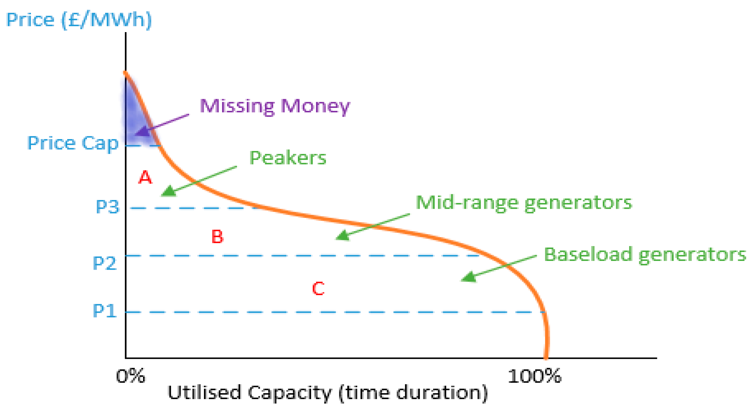
2. The Necessity for a Capacity Market

In energy-only markets, generators depend on revenues collected when exporting electricity to the grid to cover their costs. With the entrance of more intermittent renewable energy plants to the market, the energy demand increase, and the phase-out of carbon-intensive generators, the market faces a challenge to ensure energy supply adequacy. However, energy-only market neglects the energy adequacy problems because it is a price-based approach which assumes that the market always clears (quantity supplied = quantity demanded) [41,42]. This market failure along with many others resulted in the development of CMs [43]. Also, during blackouts, energy-only market is inefficient [44]. If there is a blackout in the electricity network, its duration relies on the generation capacity built to avert them. The incentive to invest in new generation capacity depends on the scarcity prices paid during blackouts. Since scarcity prices are normally capped at low price by regulators, generators may not earn sufficient revenue to recover their fixed cost and invest in building new capacity. This create the ‘missing money’ problem [45]. The other failure mechanism is that the high inelastic nature of the demand side makes customers cannot see the real-time price of electricity nor they can respond to them [46].

The missing money problem is illustrated in Figure 1 where the relationship of the spot price in the market and the utilised energy capacity as a function of time is governed by a price duration curve. This curve reflects the price change with time according to different levels of supply and demand. Peakers are operating in area A thus earning higher prices (P3 and above) but for a relatively short period of time. The mid-range generators operate for longer duration and receive the payment in areas A + B to cover the larger fixed and investment cost. The base load generators receive the payment for A + B + C. The high prices received in area A is needed to compensate all generators not just the peakers. However, the highest price in area A is normally capped low thus creating the missing money. This price cap is introduced due to administrative/regulatory procedures to protect customers from price volatility and prevent generators from exercising market power [47].

Many solutions were adopted to mitigate the missing money problem including a quantity based approach or CMs [44]. In CMs, the system operator needs to determine the optimal capacity ($C_{op}$) that could reduce/eliminate the shortage hours in the system. Then, an auction is held to determine the scarcity price needed by bidders to secure $C_{op}$. By comparing the marginal production cost with the scarcity price during the auction, bidders can decide whether to remain in or be out of the market. In effect, the auction discovers the value of the price cap needed to inform investors to build new capacity corresponding to the optimal capacity $C_{op}$.

The key here to effective CM is determining the number of expected shortage hours that correspond to ($C_{op}$). This is determined based on defining a reliability standard that optimises the loss of load expectation (LOLE) per year to 3 or 4. However, many energy regulators including OFGEM have deemed this reliability standard as inadequate in determining the real number of shortage hours or LOLE [48]. It is found in [49] that LOLE can reach 62.6 h/year in the presence of high share of renewable energy sources. Moreover, within the current market scarcity prices, it is found that LOLE can reach up to 83.3 h/year [14]. Considering the aforementioned studies, this work considers two main scenarios for LOLE to determine the battery cycling profile along the CM contract period. The first and second scenarios assume nearly 20 and 90 SSEs with different periods of 0.5 h, 1 h, 2 h and 4 h as shown in Figure 2. The distribution of the SSEs considers the peak demand periods in the recent years of Great Britain’s CM which are in quarter 1 and 4 of each year [50]. It also takes into account the probability of the duration of each shortage hours (i.e., 4 h SSE is less probable than 2 h) as presented in [30].

3. Methods

3.1. Problem Setup

In this study, the LIB is used to provide reserve services for the CM assuming 1-year contract and it cycles according to the profiles of cycling in Figure 2. During the contract’s period, the battery experiences both calendar and cycling aging that leads to capacity fade which in turn results in degradation cost. The task of a battery operator who wishes to exploit this market is to nominate a suitable capacity de-rating strategy for the battery between 0.5 h and 4 h+ [30] that can maximize revenue and minimize degradation cost. This study utilizes the LIB to get 0.5 h, 1 h, 2 h and 4 h de-rating factor as shown in

Table 1. Capacity market battery de-rating factors used in this study.

Battery Capacity (MWh)	Connection Capacity (MW)	Duration (h)
2	2	0.5
2	2	1
2	1	2
2	0.5	4

. It should be noted that the battery capacity is in Ah multiplied by the nominal voltage to get the battery capacity in MWh. The connection capacity is the power in MW in which the battery asset owner can deliver to the grid. This setup is in agreement with the current batteries participating in the CM [51]. The parameters values used in this study are given in Appendix A.

The total revenue of the battery (R), the energy losses due to degradation ($E_{lost}$) and the capacity obligation required during each SSE $C_o\left(i\right)$ are given in Equations (1)–(8).

$$R=C_{de}\times {\lambda }_{cl}\times f+R_{ov}-p$$

(1)

$$C_{de}=P_c\times k_{de}$$

(2)

$$P_c=I_b\times V_b\times N$$

(3)

$$p={\displaystyle \sum _{i=1}^n}{C}_{un\left(i\right)}\times {\lambda }_{cl}$$

(4)

$$R_{ov}={\displaystyle \sum _{i=1}^n}{C}_{ov\left(i\right)}\times {\lambda }_{cl}$$

(5)

$$E_{lost}=C_{lost\left(j\right)}\times {\lambda }_{degr}\times N$$

(6)

$$C_o\left(i\right)={\displaystyle \sum _{i=1}^n}\left(C_{de}\times D_p\left(i\right)\right)-C_b\left(i\right)$$

(7)

$$D_p\left(i\right)=\frac{D_{p\left(i\right)}^{sse}}{C_{auc}}$$

(8)

• $C_{de}$ is the de-rated capacity and $k_{de}$ is the de-rating factor
• ${\lambda }_{cl}$ and ${\lambda }_{degr}$ are the CM auction clearing price and the battery degradation cost respectively
• $f$ is a factor used to reward slightly more payment in peak demand months
• $R_{ov}$ is the CM overpayment as a result of battery discharging more than its obligation
• $p$ is the CM penalty
• $P_c$ is the battery connection capacity which is function of the battery current, voltage and the number of cells ($I_{b,}{V}_b,N$)
• $C_{un\left(i\right)}$ and $C_{ov\left(i\right)}$ are the undelivered and over delivered capacity of the obligation during settlement period (i)
• $C_{lost\left(j\right)}$ is the capacity lost as a result of battery degradation for model j
• $D_p\left(i\right)$ is the peak electricity demand during the SSE ($D_p^{sse}$) divided by the total CM contracted capacity through the CM auction ($C_{auc}$)

The meanings of the formulas are as follows:

• Equation (1) calculates the total revenue for a battery in the CM including any overpayment and penalties
• Equation (2) obtain the de-rating capacity based on the battery output power in Equation (3) and the chosen de-rating strategy (i.e., 0.5 h, 1 h etc.)
• Equation (4) calculates the penalty of the battery by multiplying any undelivered capacity obligation by the CM’s auction clearing price. The amount of undelivered capacity is calculated based on the battery’s State of Charge (SoC) at the end of any SSE.
• Equation (5) calculates the overpayment similar to (4)
• Equation (6) calculates the battery capacity degradation cost by multiplying the cell degradation by the cost of degradation along with the number of cells
• Equation (7) calculates the capacity obligation that must be delivered by the battery considering the duration of the SSE(i) and peak demand in Equation (8) minus any delivered balancing services capacity

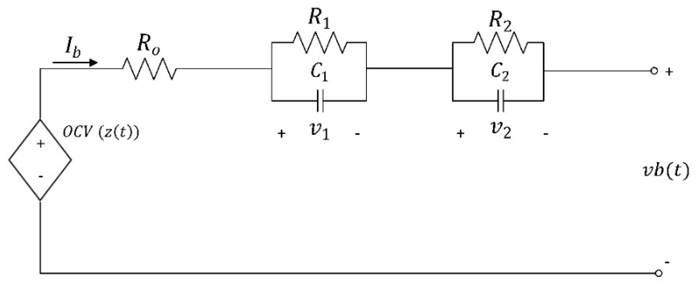
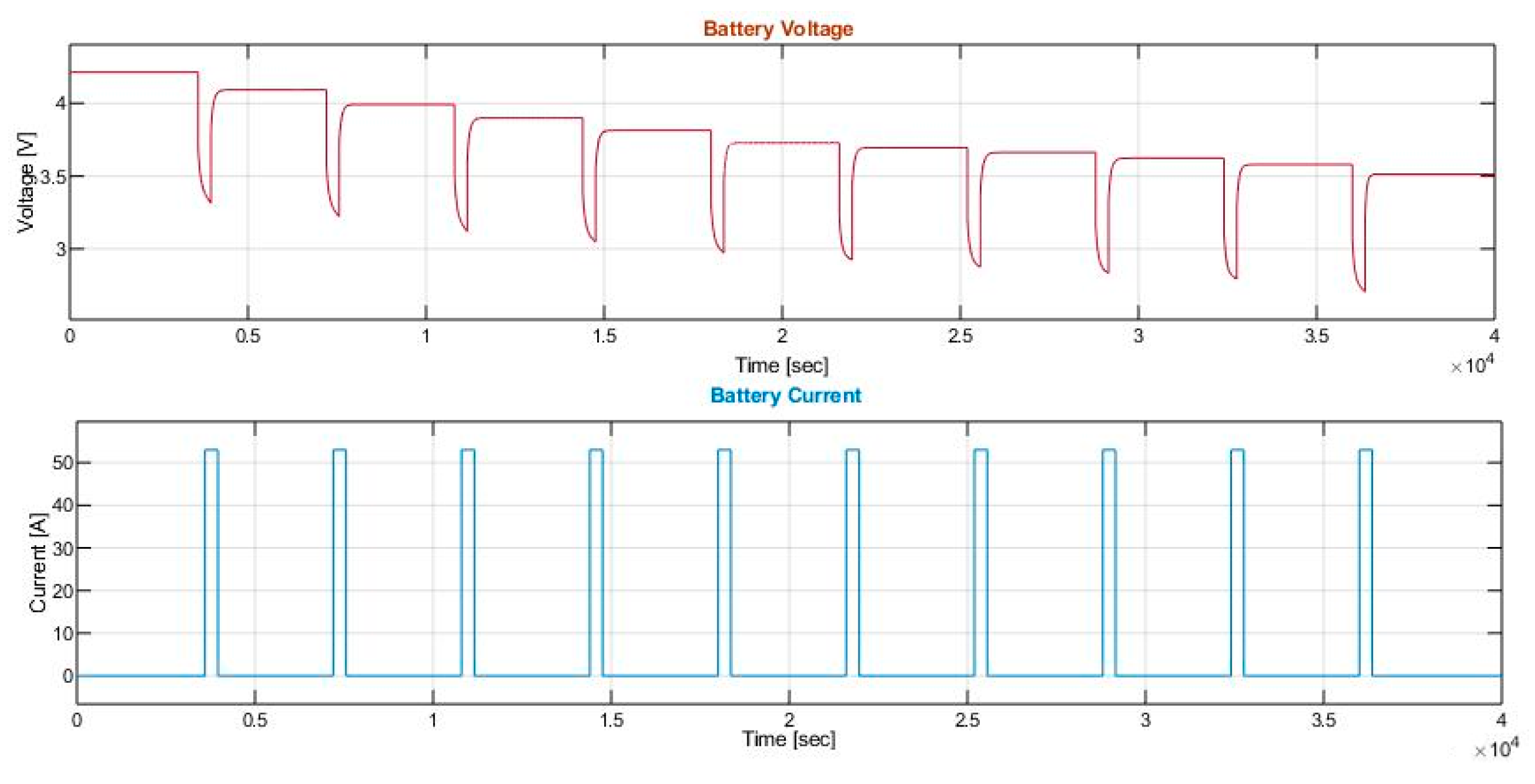
3.2. Equivalent Circuit Battery Model

One LIB cell with a capacity of 53 Ah is simulated by using equivalent circuit battery model (ECM) as shown in Figure 3. The 53 Ah cell then scaled to 2 MWh battery that contain 10,080 cells. Both the revenue and degradation cost are then multiplied by the number of cells. This assumes a high-quality cell balancing and battery management system in which all cells behave equally such that each cell is controlled individually as in [20,52,53]. The purpose of the battery model is to update the capacity of the battery continuously after the cycling to get accurate SoC value to estimate the CM penalties ($p$). The model may be not needed for such analysis if the battery tested online and was fed into the degradation model to obtain the lifetime analysis. In this model, $R_o$ is the ohmic resistance that represents charge/discharge energy losses. $R_1$ and $C_1$ describe the charge transfer resistance and double layer capacitance respectively while $R_2$ and $C_2$ are used to capture battery diffusion effects. A detailed presentation and discussion of the model can be found in [54,55,56].

The electrical behavior of the battery is expressed in (9)–(12):

$$\frac{d{i}_{R1}}{dt}=-\frac{1}{R_1{C}_1}{i}_{R1}\left(t\right)+\frac{1}{R_1{C}_1}{i}_b\left(t\right)$$

(9)

$$\frac{d{i}_{R2}}{dt}=-\frac{1}{R_2{C}_2}{i}_{R2}\left(t\right)+\frac{1}{R_2{C}_2}{i}_b\left(t\right)$$

(10)

$$\frac{d\mathrm{z}\left(t\right)}{dt}=\mathrm{z}\left(t_o\right)-\frac{\mathsf{ƞ}}{3600C_N}\int i_b\left(t\right)$$

(11)

$$v\left(t\right)=OCV\left(\mathrm{z}\left(t\right)\right)-v_1\left(t\right)-v_2\left(t\right)-R_o{i}_b\left(t\right)$$

(12)

Since the ECM uses a coulomb counting method for SoC estimation in (11) which suffers from errors if the initial capacity was not correctly determined, the battery capacity was continuously updated by the degradation model similar to [57]. The battery parameters are presented in

Table 2. Battery model parameters for Li-ion NMC cell at T = 20 °C.

SoC	OCV (V)	R0 (mΩ)	R1 (mΩ)	C1 (kF)	R2 (mΩ)	C2 (kF)
0	3.5136	9.6145	4.944	9.792	0.746	27.958
0.1	3.579	9.3483	4.928	12.621	0.572	38.512
0.2	3.623	9.5188	4.925	14.635	0.507	37.631
0.3	3.662	9.4834	4.90	15.301	0.498	26.237
0.4	3.694	9.4206	4.878	13.912	0.270	20.286
0.5	3.727	9.3673	4.899	11.905	0.0032	18.975
0.6	3.813	9.356	4.890	14.256	0.2385	15.288
0.7	3.899	9.3326	4.889	14.488	0.556	16
0.8	3.991	9.3847	4.884	13.775	0.288	18.763
0.9	4.092	9.240	4.822	15.166	0.659	18.454
1	4.21	9.351	4.885	12.889	0.490	12.412

which are fitted based on the experimental data in [58] using nonlinear least square algorithm. Figure 4 shows the simulation results for battery current and voltage taking SoC steps from 0 to 1 which accurately corresponds to the data presented in [58].

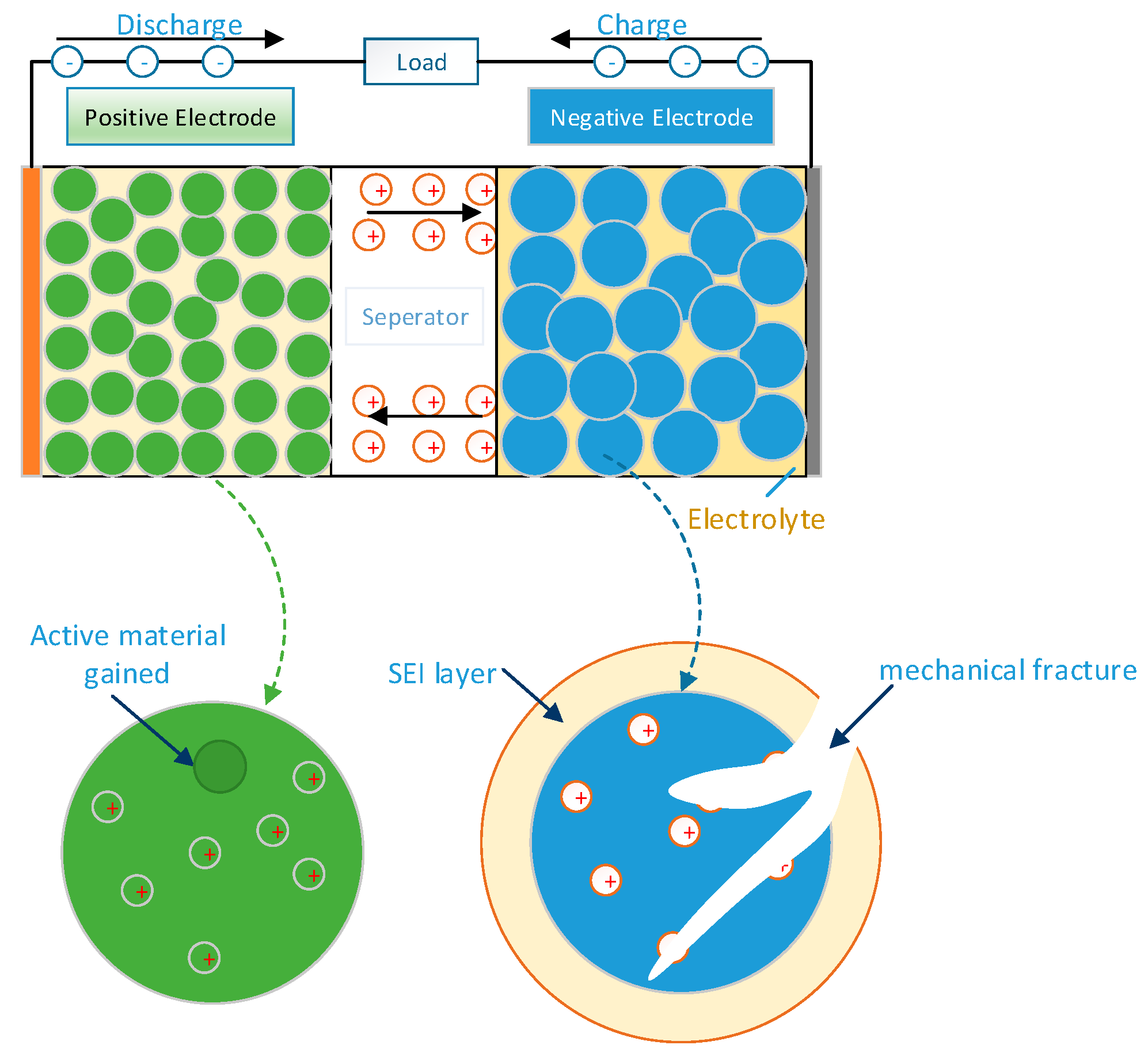
3.3. Degradation Models

LIB’s capability to store energy decreases over time resulting in capacity fade, power fade or both. This is as a result of complex electrochemical and mechanical processes inside the battery that can take place simultaneously [40]. These degradation mechanisms are influenced by the operating conditions. During battery cycling, the degradation rate is influenced by C-rate, cycle depth effect (DoD), and temperature [59]. In storage condition, the degradation rate is influenced by temperature, idle time and SoC [60]. The purpose of battery degradation models, therefore, is to predict the battery lifetime considering these influencing parameters. Both battery degradation models below as well as the ECM model use the same battery chemistry (NMC) [33].

The power fade results in the battery’s resistance increase which in turn leads to capacity decrease. However, because there is not a quantifiable measure that link resistance increase to capacity decrease for cost modelling purposes, we assumed that the battery resistance increase is an indicative factor to degradation and eventually the capacity decrease will be used to quantify the nominal capacity in this paper.

3.3.1. Empirical Model

In this model, a large set of battery degradation experimental data is interpolated by empirical or parametric functions. In the experimental study presented by Schmalstieg et.al. [61], 42 LIB cells were stored for 500 days at different temperatures and voltages (SoCs) to increase reproducibility and the accuracy of the calendar aging model. Similarity, 22 cycle aging tests with different DoDs and mean SoC were tested to produce cycling aging model. Then the experimental data was mathematically fitted in several steps to represent a lifetime degradation model. For the calendar aging model, the capacity reduction ($C_{cal}$) over the number of days $\left(d\right)$ is represented by a ($d^{0.75}$) function with a degradation fitting parameter $\left(\alpha \right)$ as in (13). Then $\alpha$ is used to capture the SoC dependency (V) via a linear relationship (14) and temperature dependency (T) via Arrhenius Equation (15). The resultant $\left(\alpha \right)$ is given in (16) [61].

Similarly, the cycling aging model captures the capacity reduction ($C_{cyc}$) over the number of equivalent full cycles ($Nc$) based on ($t^{0.5}$) function with a degradation fitting paramter $\left(\beta \right)$ as in (17). Then $\beta$ is used to capture cycle depth effect (DoD) and the average voltage ($V_{av}$). Therfore, the total cycling and calendar aging model used in this study is given in (18) [61].

$$C_{cal}=\alpha ·d^{0.75}$$

(13)

$${\alpha }_v\left(v\right)=a+b·V_b\left(t\right)$$

(14)

$${\alpha }_T\left(\mathrm{T}\right)=a1·\exp (\frac{-E_A}{RT})$$

(15)

$$\alpha \left(T,V\right)=(7.543·V_b\left(t\right)-23.75)·{10}^6·e^{\frac{-6976}{T}}$$

(16)

$$C_{cyc}=\beta ·N{c}^{0.5}$$

(17)

$$C_{lost1}=\left(\alpha \left(V_b\left(t\right),T\right)·d^{0.75}+\beta \left(DoD,V_{mean}\left(t\right)\right)\times \sqrt{\int 2I_b\left(t\right)}\right)$$

(18)

3.3.2. Semi-Empirical Model

Semi-empirical models develop on the empirical ones by including theoretical basis for some degradation mechanisms. For instance, this model can capture the battery cycling temperature dependency which was not captured in the empirical mode. Therefore, they partly reduce the need for gathering considerable amount of experimental data needed in the empirical models [62]. One example of such models is developed by Smith et.al [63] in which 12 LIB cells were tested at different SoCs, DoDs, and temperatures. In this model, three degradation mechanisms inside a LIB cell are represented in Figure 5. First, it is assumed that some lithium particles at the interphase between the electrolyte and the negative electrode are prevented from contributing to the main chemical reaction due to the formation of solid electrolyte interphase (SEI) layer. This SEI layer grows with time and together with the mechanical fracture occurred due to minimum battery cycling results in capacity fade ($Q_{SEI}$) as in (19). In (19), $d{0}_{T\left(t\right)}$ captures the battery temperature dependency based on Arrhenius formula for all the mechanisms. Then, the first term in (19) captures SEI layer growth with time, the second term captures the battery loss with mild cycles and the third term captures the beginning of capacity loss in the first cycle/day. With more expansion and contraction of electrode materials during charging/discharging, the negative electrode particles face increased stress that lead to mechanical fracture which results in active material loss ($Q_{AM}$) in (20). Equation (20) assumes that there is a negative electrode active material loss with every cycle ($N_c$). Third, at the cell’s beginning of life, the positive electrode storing capability ($Q_{pos}$) will slightly increase because it is found that temperature is the main controlling factor in the first few cycles leading to an increased Ah throughput in (21). The total capacity loss is governed by (22) and all model parameters are from [63] which are given in MATLAB code with the Supplementary Materials.

$$\begin{array}{c}{Q}_{SEI}=d{0}_{T\left(t\right)}(b_0-b_1\left(T\left(t\right),SoC\left(t,T\right),DoD\right)·d^{0.5}-b_2\left(T\left(t\right),OCV\left(t,T\right),DoD\right)\\ ·N_c-b_3(T\left(t\right)·\left(1-\exp (-\mathrm{d}/{\tau }_{b3}\right)\end{array}$$

(19)

$$\frac{\mathrm{d}{Q}_{AM}}{\mathrm{d}{N}_c}=-\frac{c_1\left(T\left(t\right),DoD\right)}{Q_{AM}}$$

(20)

$$Q_{pos}=d{0}_{T\left(t\right)}+(d_3·\left(1-\exp (-\int \frac{2I_b\left(t\right)}{228})\right)$$

(21)

$$C_{lost2}=\min \left(Q_{SEI},Q_{AM},Q_{pos}\right)$$

(22)

3.4. Degradation Cost

Although the general trend of battery pack cost is decreasing, there is no unified way for estimating battery pack cost precisely for any system because the cost is rarely disclosed publicly [64]. Moreover, the cost would depend on the owner’s preference for battery chemistry, lifetime, power electronics equipment, thermal management system, the quality of battery management system amongst other factors. As such, the battery pack cost is subject to great uncertainty. Some studies assumed a battery pack cost of 125 $/kWh by 2022 [65]. Other study found that the minimum battery pack price is 220 €/kWh in 2018 [66]. This study considers Bloomberg analyses for battery pack price of 176 $/kWh in 2019 [67] which we assumed that it includes the cost of all BMS components such as the thermal management system reviewed in [21]. As such, the degradation cost is set to 0.5 £/Ah by assuming a constant average voltage of 3.65 V similar to [28].

4. Results

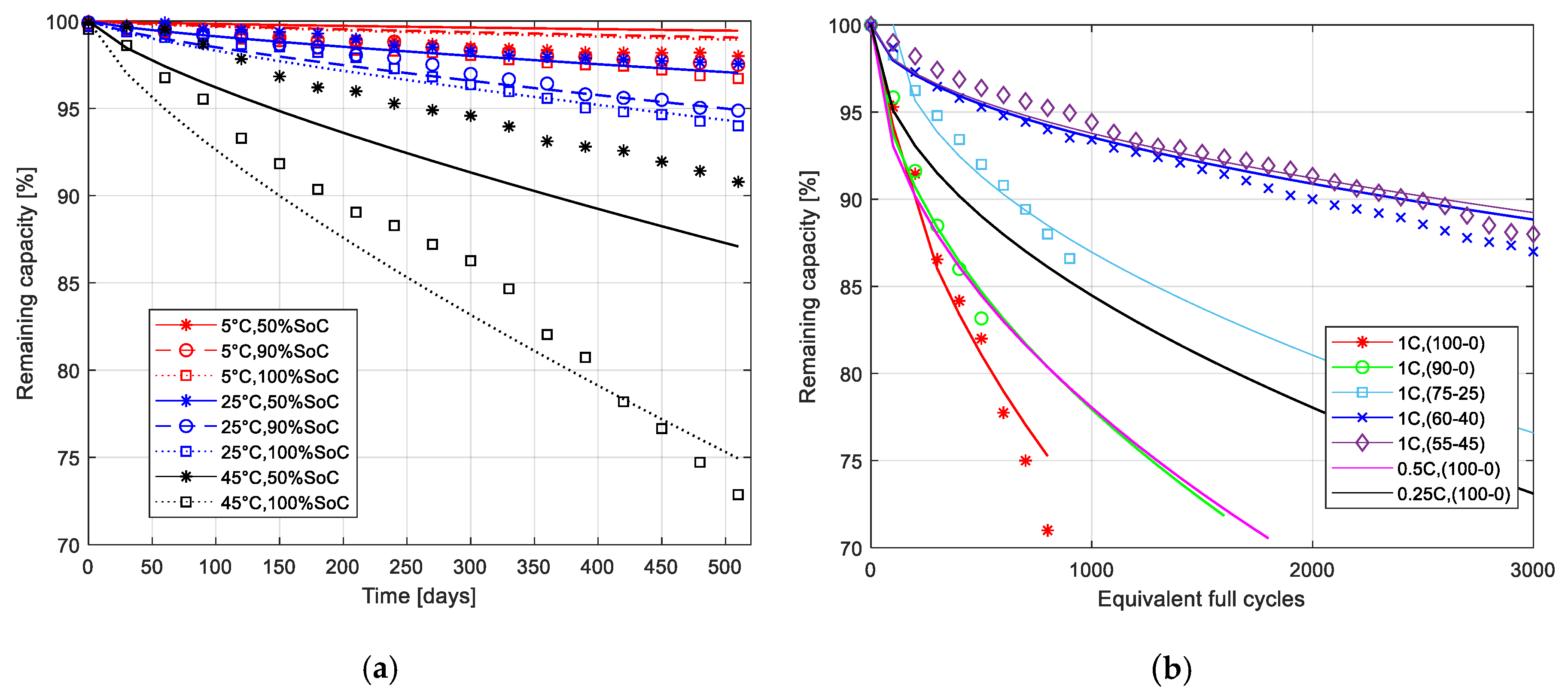
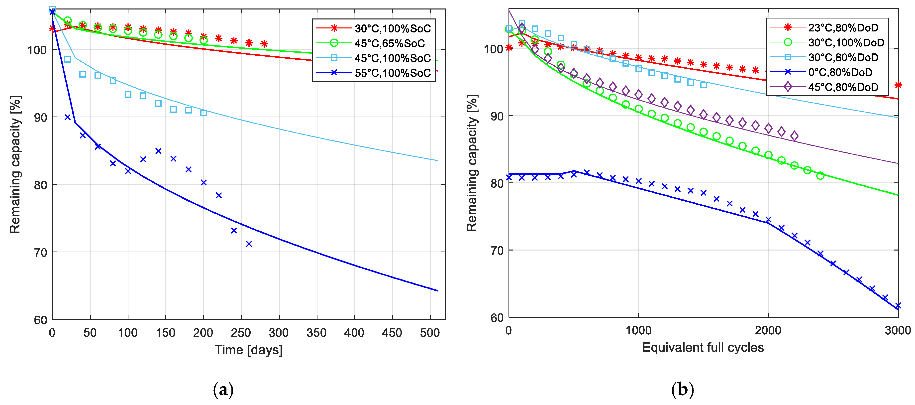
4.1. Accuracy of Battery Degradation Models

The calendar and cycle degradation for the empirical model as predicted by (18) along with the corresponding experimental data are presented in Figure 6a,b. Figure 6a shows the calendar aging results at different temperatures and SoCs where degradation is exacerbated by increasing temperature and SoCs. The model shows good accuracy when compared by the same experiment data sets provided by [61]. It also corresponds well to the calendar experimental data for the NMC battery cell provided by [68] which is presented here. This shows that the calendar aging results may be valid outside the operating conditions firstly tested using $t^{0.5}$ or $t^{0.75}$ functions [69]. Figure 6b shows the cycling results at different C-rates and DoDs where capacity loss is high at higher DoD and C-rate.

Figure 7a,b shows the calendar and cycle degradation for the semi-empirical model as predicted by (22) along with the corresponding experimental data. Figure 7a shows that this NMC cell experienced minimum degradation at 30 °C, 100%SoC and 45 °C, 65%SoC. The 55 °C, 100%SoC cell experienced severe and nonlinear degradation which indicate the higher temperature can lead to unexpected battery behaviour. When it is needed to perform a reference capacity testing for the 55 °C, 100%SoC cell, it was cycled above the recommended temperature set by the manufacturer thus the reference performance tests were done at 45 °C which explains the divergence of the results compared to the model [63]. Figure 7b shows increased capacity fade at higher DoD. It shows also that maximum degradation is at 0 °C, 80%DoD in which the cell starts at 81% of its capacity without any degradation. The reduction in capacity at very low temperatures may be related to changes of the electrode materials and separator structures [70] or to the difference in pressure experienced by negative and positive electrodes [71].

Table 3. Maximum root mean square error [%] for both empirical and semi-empirical models.

Degradation Type	Empirical RMSE [%]	Semi-Empirical RMSE [%]
Calendar	3.4	4.9
Cycle	1.7	1.1

shows the maximum root mean square error for the simulations of Figure 6 and Figure 7.

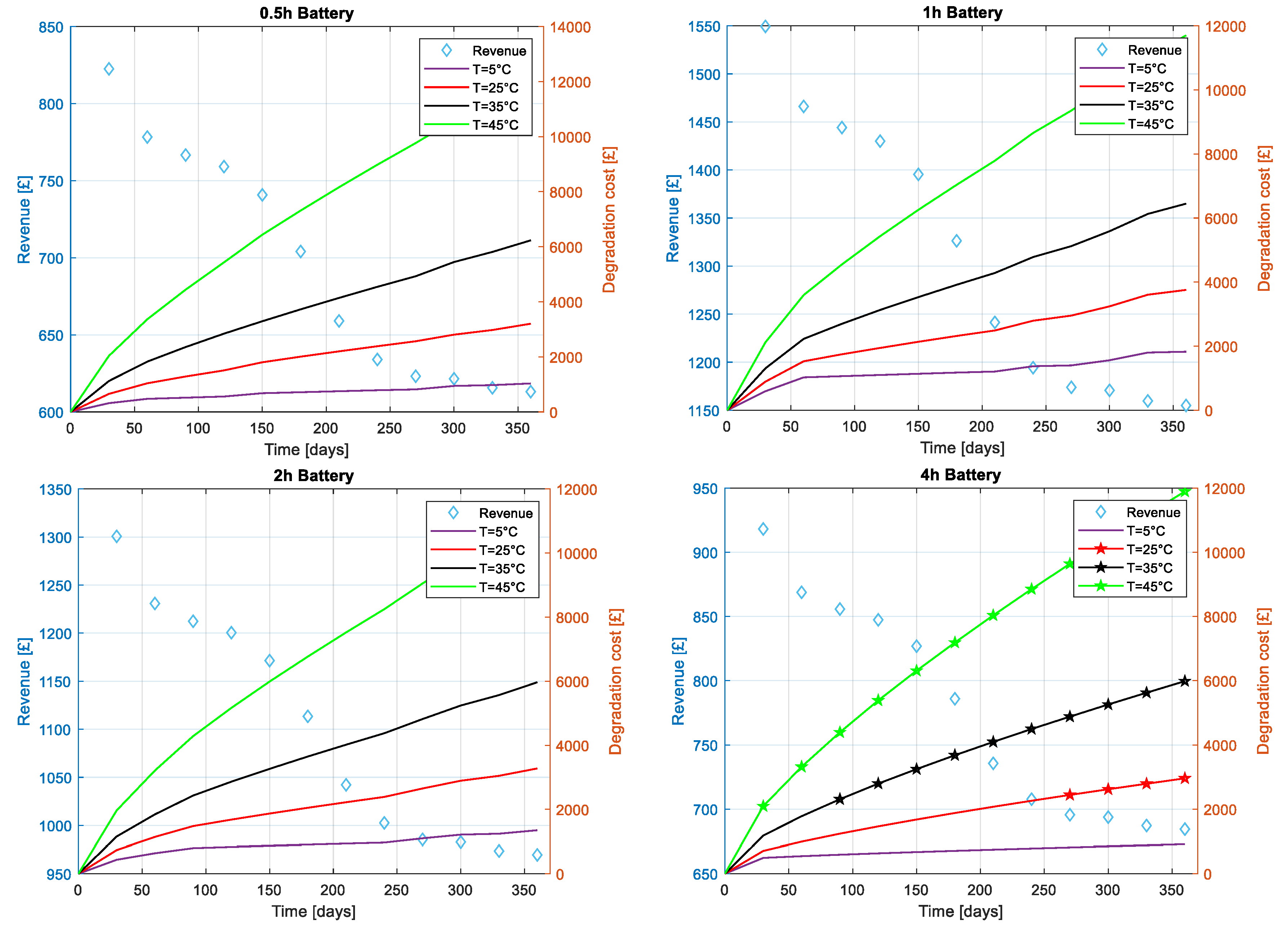
4.2. Revenue and Degradation Cost in the Capacity Market

This section presents the revenue and degradation cost for each battery at 0.5 h, 1 h, 2 h and 4 h de-rating factors. Here the cycling is according to scenrario1 in Figure 2a. Since the cycling in the CM is generally low, we assumed that once the SSE occurs, the battery will be fully charged based on the present SoC (i.e., if the battery is left at 50%SoC to reduce calendar aging, then it should be charged to 100%SoC). This assumption consider the fact that the battery in the CM has 4 h notice to deliver the required capacity obligation which is enough for fully charging the battery [30].

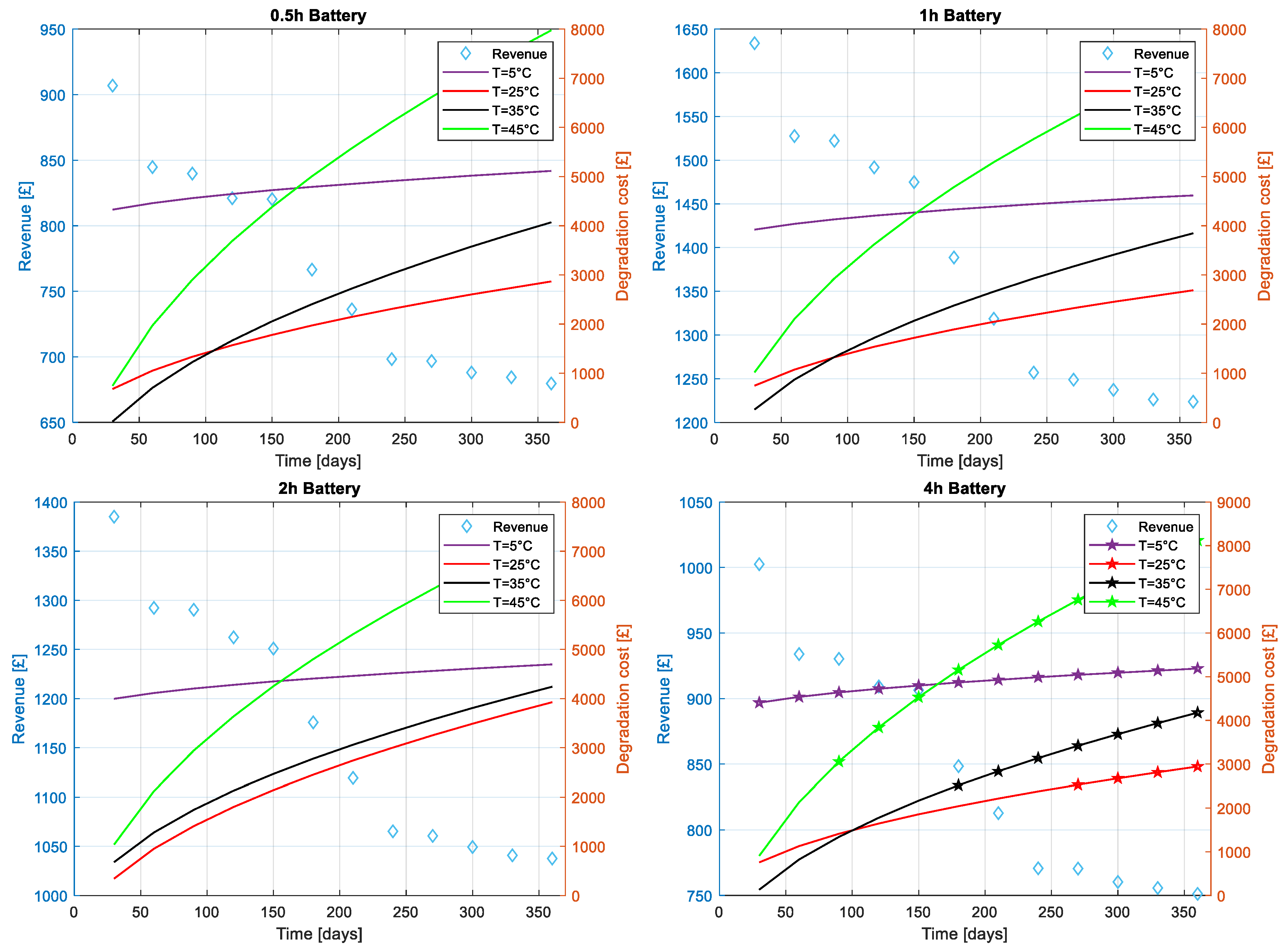
4.2.1. Revenue and Degradation Cost for Different Temperatures

The revenue and the degradation cost for the four batteries along 1 year CM contract are depicted in Figure 8 and Figure 9. The capacity fade calculation uses the empirical model (18) and the semi-empirical model (22) in Figure 8 and Figure 9 respectively. In Figure 8, in general, the degradation cost increases by increasing the temperature from 5 °C to 45 °C. At 5 °C, The battery with the 2 h de-rating factor receives the highest profit (revenue–degradation cost) because it discharges its de-rated capacity with a lower current rate (0.5) and receives a relatively high de-rating factor. Therefore, it is recommended in this case to optimise the battery to get 2 h de-rating factor with 5 °C storing temperature.

Figure 9 shows slightly higher revenues for all the batteries due increased battery capacity ($Q_{pos}$) predicted in the first days/cycles. It also shows, in contrast to Figure 8, that degradation cost is maximum at T = 5 °C and minimum at T = 25 °C. This is because unlike the empirical model, the semi-empirical model assumes that the SEI layer formation occurs not only because calendar aging but also accounts for mild cycles (see Section 3.3.2). At T = 25 °C, the 1 h battery shows the highest profit. The semi-empirical model predicts lower capacity fade per temperature if compared to the empirical model. For instance, the degradation cost can reach up to £6000 for all the batteries in Figure 8 while it is nearly 4000 £ in Figure 9.

Two general trends can be noticed in both Figure 8 and Figure 9. First, the number of the incurred penalties for the 4 h battery is high because the remaining battery capacity will not be sufficient to account for the capacity obligation predicted by (7) in all of the 4 h SSE. Second, the 1 h and 2 h batteries receive the highest revenue respectively because they discharge high de-rated capacity and receive less penalties compared to the 0.5 h and 4 h batteries.

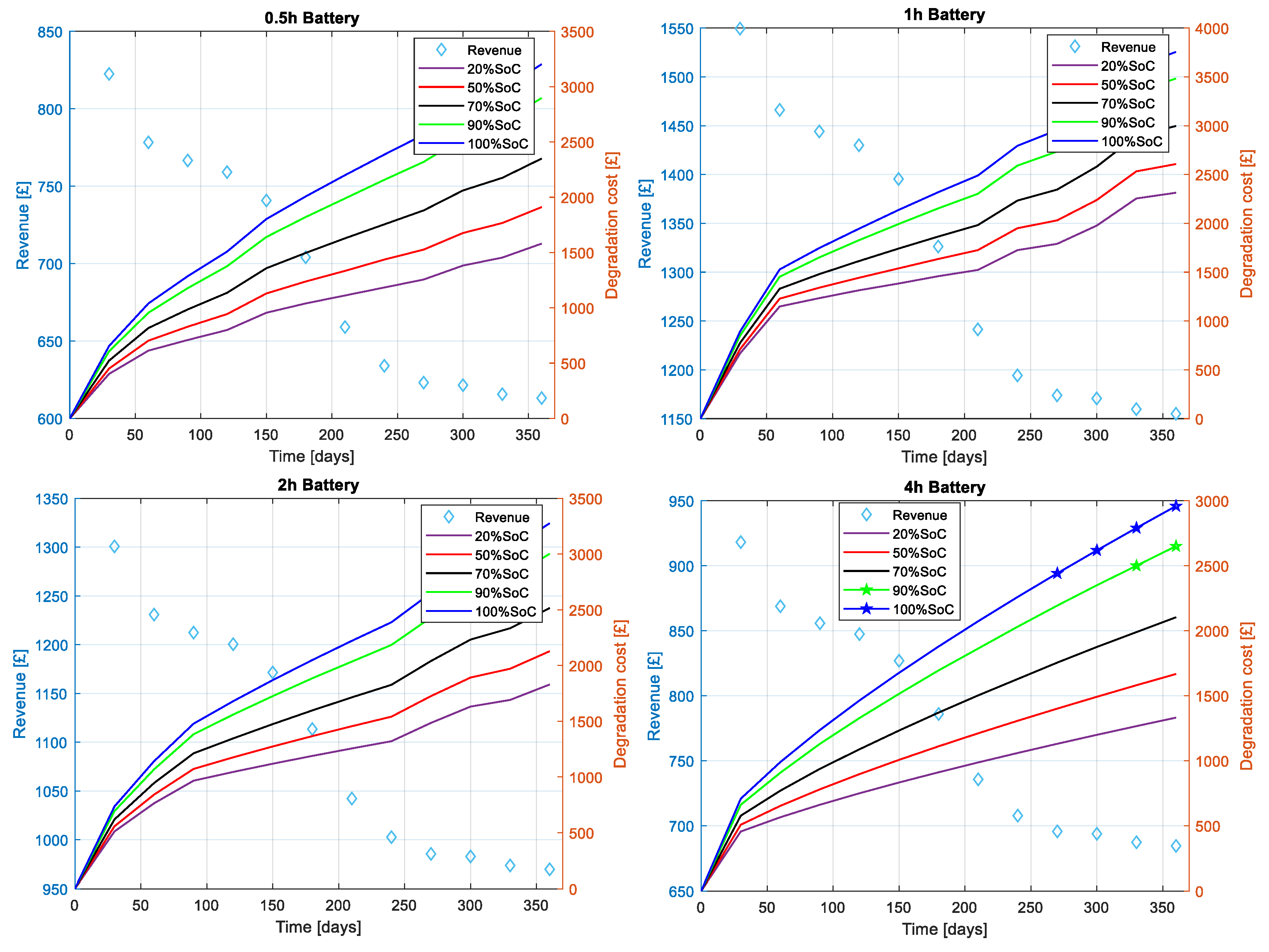
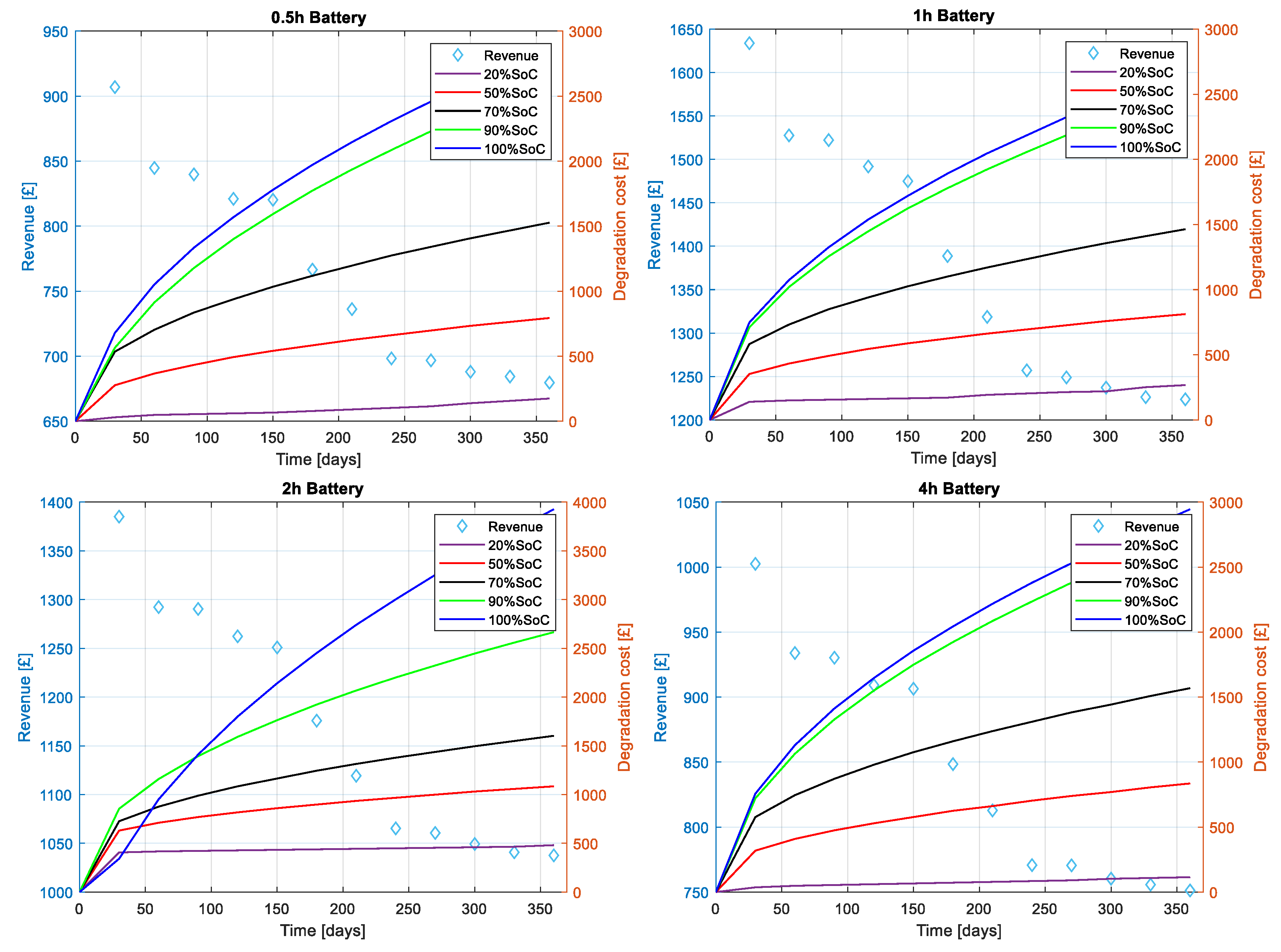
4.2.2. Revenue and Degradation Cost for Different SoCs

Figure 10 and Figure 11 show the revenue and degradation cost for different SoCs with the temperature is constant at 25 °C for all the batteries. This assumes that the battery asset owner can control the temperature using thermal management system. Then, the battery can get charged when the 4-h notice from the system operator is received. The capacity fade calculation uses the empirical model (18) and the semi-empirical model (22) in Figure 10 and Figure 11 respectively. The general trend in both figures is that the higher the SoC the lower the overall profit. Therefore, the battery should be maintained at lower SoC to reduce capacity fade in the CM. However, if the battery is contracted to deliver other balancing services while a SSE occurs at the same time, this may compromise the contract or make the battery capacity insufficient to deliver its CM obligation. Moreover, both figures show the 2 h battery generally offer the highest overall profit amongst the four batteries if all the SoC range (20–100%) is taken on average.

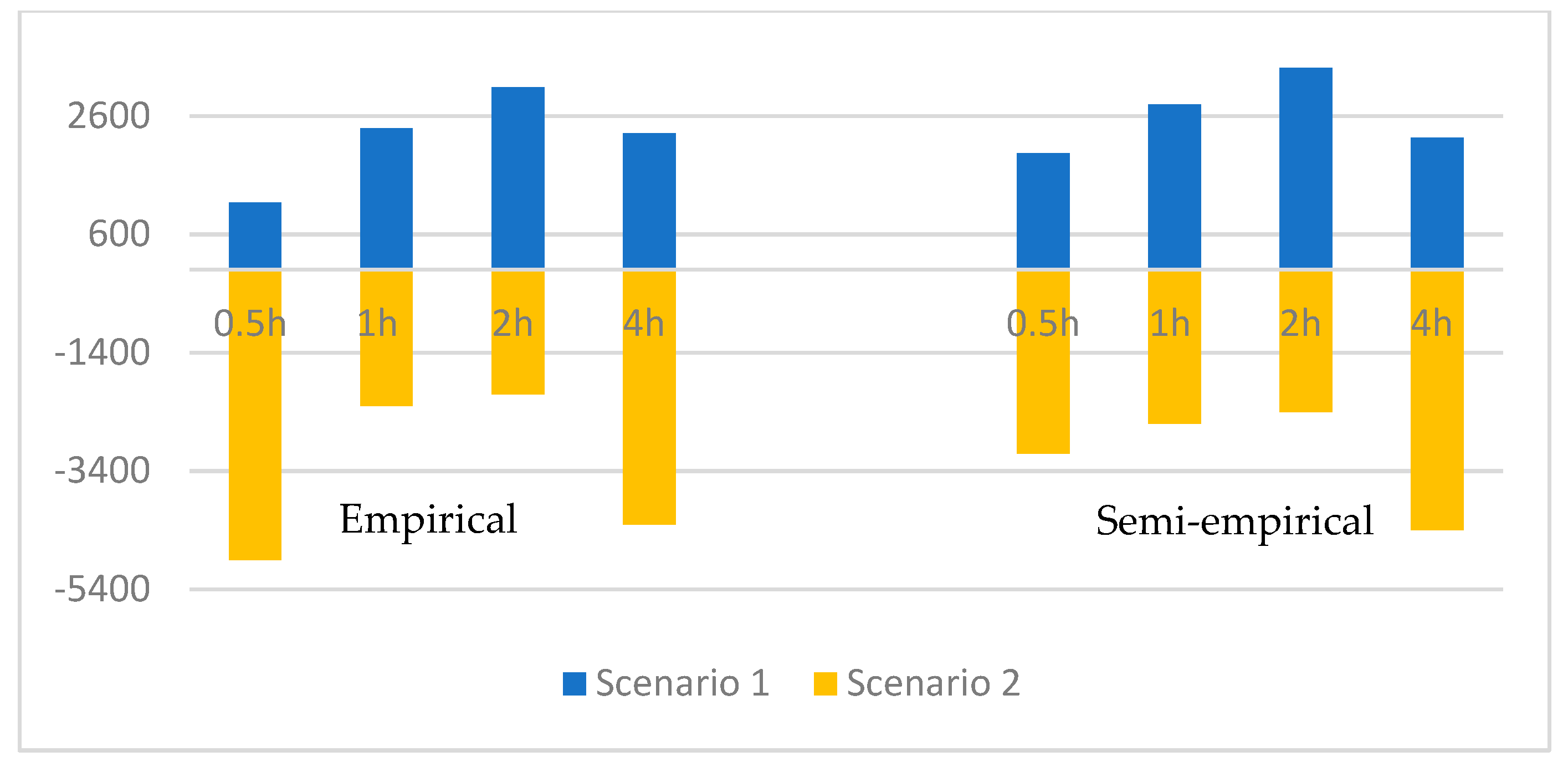
4.3. Increased Battery Cycling Effects

The total profit of the four batteries at the end of the CM contract for both scenarios in Figure 2 is shown in Figure 12. This assumes an ideal case for both empirical (T = 5 °C) and semi-empirical models (T = 25 °C). It can be clearly shown that with increased cycling or increased SSEs, providing CM services is not economically viable for all batteries. Increasing the LIB capacity can be one of the solutions to make providing longer term backup service to the grid cost effective. However, this presents also an opportunity to other longer-duration energy storage technologies such as flow batteries which has longer cycle life than LIB to increase grid resiliency [72].

5. Discussion

Two policy recommendations arise from this work. First, degradation cost either needs to be remunerated or accounted for in the CM regulations in such a way to reduce the exposure to penalties. This is because by using all models and scenarios, degradation cost can substantially reduce the overall profit in the CM. For instance, if an ideal case is used by assuming the battery’s temperature is at T = 5 °C and 20% SoC, then the empirical model predicts that the degradation cost account for nearly 53% of the overall revenue in 1 year. Also, the semi-empirical model predicts the ideal case will result in 9% degradation cost of the overall revenue in 1 year. However, to the best of our knowledge, no CM in the world remunerates the battery degradation cost but at the same time penalize battery owners for any shortage in the capacity obligation. Second, CMs should provide the necessary overpayments for batteries. The current CM regulations provide overpayment—in case the battery discharged more than its capacity obligation—only if there are penalties collected from different CM units that did not deliver. However, since the capacity obligation always takes into account the de-rated capacity as in (7) which in most cases lower than the original battery capacity, the battery will always over deliver as it is required to fully discharge the battery once the SSE occur. For these previous reasons along with fuel neutrality in the CM, the current CMs design may be ill suited to incentivize low carbon resources and secure energy supply [73].

Three limitations also arise from this study. First, degradation models can be outdated because all degradation models need to be fitted based on the experimental battery data which has changed hugely over the years due to the advancement in battery materials. For example, the capacity fade in a more recent work for the NMC battery cell can be only around 7% after 4500 cycles and less than 1% after 450 day [74]. Second, a battery asset owner can utilise the battery to provide many other different ancillary services which is not considered in this study. Third, both empirical and semi-empirical models either underestimate or overestimate the total degradation at 5°C. The experimental data at T = 5 °C for the same NMC cell shows that the calendar degradation is minimum at 5 °C while the cycling degradation is maximum [68]. This necessitates the need for a high fidelity physics based degradation model in order for the degradation cost analysis be more accurate. The computational cost for such models depends on many factors such as the final application requirements, the assumptions used to reduce the model order, and the number of degradation mechanisms considered. For a lifetime cost study that is done offline then the computational cost will not be a problem and the overall goal becomes to inform the cost–benefit analysis before the actual battery opts for a service contract. In the CM application and since the battery owner has 4 h to discharge, then if it needed to check the state of health of the battery online, it is essential that the computational cost be less than 4 h. In other balancing services for example that requires response within 10 minutes’ notice, then a simplification of the physics model is required as in [37]. Detailed discussion about the computational efficiency for physics based model are presented in [75].

6. Conclusions

In this work, an equivalent circuit battery model with a capacity of 2 MWh coupled with empirical and semi-empirical degradation models was used to provide backup service in the CM along one year. The accuracy of the battery model and the degradation models were tested by comparing them with the corresponding experimental data. Then by controlling the battery’s output power, this battery is utilised to get four capacity de-rating factors of 0.5 h, 1 h, 2 h and 4 h to study which strategy can maximize the overall revenue. During the CM contract, the battery experiences both cycle and calendar capacity fade which result in a degradation cost. To account for the number of shortage hours in one year in the CM, two battery cycling scenarios were created based on the historical energy demand data in Great Britain and earlier research.

The results illustrate that the 2 h and 1 h batteries get the highest revenue in all the simulated scenarios. Also, degradation cost can significantly impact the potential profit by using each de-rating strategy if the battery storing temperature is not correctly controlled. The empirical degradation model predicts that battery degradation is minimum at lower temperatures such as 5 °C. The semi-empirical model predicts that battery degradation is minimum at the standard temperature 25 °C. This is because each model quantify degradation differently. Moreover, by using both degradation models, keeping the battery at lower charge levels results in less capacity fade. While providing CM service may be economically viable when the number of shortage hours per year are low, it becomes not profitable if these shortage hours increase.

The impact of battery degradation on other services profitability together with the CM could be studied in the future using physics-based battery degradation model that can mitigate the limitation of the empirical and semi-empirical model especially at lower temperatures such as 5 °C.

References

1. IRENA. Renewable Capacity Highlights; International Renewable Energy Agency: Abu Dhabi, UAE, 2019; Available online: https://bit.ly/2IaRs78 (accessed on 10 October 2019).
2. BEIS. UK Renewable Electricity Capacity and Generation; Department for Business Energy & Industrial Strategy: London, UK, 2019. Available online: https://bit.ly/31y7gXz (accessed on 2 September 2019).
3. Kerdphol, T.; Watanabe, M.; Mitani, Y.; Phunpeng, V. Applying Virtual Inertia Control Topology to SMES System for Frequency Stability Improvement of Low-Inertia Microgrids Driven by High Renewables. Energies 2019, 12, 3902. [Google Scholar] [CrossRef] [Green Version]
4. Sandelic, M.; Sangwongwanich, A.; Blaabjerg, F. Reliability Evaluation of PV Systems with Integrated Battery Energy Storage Systems: DC-Coupled and AC-Coupled Configurations. Electronics 2019, 8, 1059. [Google Scholar] [CrossRef] [Green Version]
5. Williams, S.; Short, M.; Crosbie, T. On the use of thermal inertia in building stock to leverage decentralised demand side frequency regulation services. Appl. Therm. Eng. 2018, 133, 97–106. [Google Scholar] [CrossRef] [Green Version]
6. Hossain, M.S.; Madlool, N.A.; Rahim, N.A.; Selvaraj, J.; Pandey, A.K.; Khan, A.F. Role of smart grid in renewable energy: An overview. Renew. Sustain. Energy Rev. 2016, 60, 1168–1184. [Google Scholar] [CrossRef]
7. Yoon, M.; Lee, J.; Song, S.; Yoo, Y.; Jang, G.; Jung, S.; Hwang, S. Utilization of Energy Storage System for Frequency Regulation in Large-Scale Transmission System. Energies 2019, 12, 3898. [Google Scholar] [CrossRef] [Green Version]
8. Chattopadhyay, D.; Alpcan, T. Capacity and Energy-Only Markets under High Renewable Penetration. IEEE Trans. Power Syst. 2016, 31, 1692–1702. [Google Scholar] [CrossRef]
9. UK Government. 2010 to 2015 Government Policy: UK Energy Security; Department of Energy & Climate Change: London, UK, 2014.
10. Spees, K.; Newell, S.A.; Pfeifenberger, J.P. Capacity Markets—Lessons Learned from the First Decade. Econ. Energy Environ. Policy 2013, 2, 1–26. [Google Scholar] [CrossRef]
11. Federal Ministry for Economic Affairs and Energy. System Adequacy for Germany and its Neighbouring Countries: Transnational Monitoring and Assessment; Consentec: Berlin, Germany, 2015. [Google Scholar]
12. Bublitz, A.; Keles, D.; Zimmermann, F.; Fraunholz, C.; Fichtner, W. A survey on electricity market design: Insights from theory and real-world implementations of capacity remuneration mechanisms. Energy Econ. 2019, 80, 1059–1078. [Google Scholar] [CrossRef]
13. Mastropietro, P.; Rodilla, P.; Batlle, C. National capacity mechanisms in the European internal energy market: Opening the doors to neighbours. Energy Policy 2015, 82, 38–47. [Google Scholar] [CrossRef]
14. Bhagwat, P.C.; Marcheselli, A.; Richstein, J.C.; Chappin, E.J.L.; De Vries, L.J. An analysis of a forward capacity market with long-term contracts. Energy Policy 2017, 111, 255–267. [Google Scholar] [CrossRef]
15. Forrester, S.P.; Zaman, A.; Mathieu, J.L.; Johnson, J.X. Policy and market barriers to energy storage providing multiple services. Electr. J. 2017, 30, 50–56. [Google Scholar] [CrossRef]
16. Ibrahim, H.; Ilinca, A.; Perron, J. Energy storage systems—Characteristics and comparisons. Renew. Sustain. Energy Rev. 2008, 12, 1221–1250. [Google Scholar] [CrossRef]
17. Pandžić, H.; Wang, Y.; Qiu, T.; Dvorkin, Y.; Kirschen, D.S. Near-Optimal Method for Siting and Sizing of Distributed Storage in a Transmission Network. IEEE Trans. Power Syst. 2015, 30, 2288–2300. [Google Scholar] [CrossRef]
18. Wang, L.; Liang, D.H.; Crossland, A.F.; Taylor, P.C.; Jones, D.; Wade, N.S. Coordination of Multiple Energy Storage Units in a Low-Voltage Distribution Network. IEEE Trans. Smart Grid 2015, 6, 2906–2918. [Google Scholar] [CrossRef] [Green Version]
19. Gayme, D.; Topcu, U. Optimal power flow with large-scale storage integration. IEEE Trans. Power Syst. 2013, 28, 709–717. [Google Scholar] [CrossRef] [Green Version]
20. Engels, J.; Claessens, B.; Deconinck, G. Techno-economic analysis and optimal control of battery storage for frequency control services, applied to the German market. Appl. Energy 2019, 242, 1036–1049. [Google Scholar] [CrossRef] [Green Version]
21. Hesse, C.H.; Schimpe, M.; Kucevic, D.; Jossen, A. Lithium-Ion Battery Storage for the Grid—A Review of Stationary Battery Storage System Design Tailored for Applications in Modern Power Grids. Energies 2017, 10, 2107. [Google Scholar] [CrossRef] [Green Version]
22. Goebel, C.; Hesse, H.; Schimpe, M.; Jossen, A.; Jacobsen, H. Model-Based Dispatch Strategies for Lithium-Ion Battery Energy Storage Applied to Pay-as-Bid Markets for Secondary Reserve. IEEE Trans. Power Syst. 2017, 32, 2724–2734. [Google Scholar] [CrossRef]
23. Khan, A.S.M.; Verzijlbergh, R.A.; Sakinci, O.C.; De Vries, L.J. How do demand response and electrical energy storage affect (the need for) a capacity market? Appl. Energy 2018, 214, 39–62. [Google Scholar] [CrossRef]
24. Staffell, I.; Rustomji, M. Maximising the value of electricity storage. J. Energy Storage 2016, 8, 212–225. [Google Scholar] [CrossRef] [Green Version]
25. Castagneto Gissey, G.; Dodds, P.E.; Radcliffe, J. Market and regulatory barriers to electrical energy storage innovation. Renew. Sustain. Energy Rev. 2018, 82, 781–790. [Google Scholar] [CrossRef]
26. Rappaport, R.D.; Miles, J. Cloud energy storage for grid scale applications in the UK. Energy Policy 2017, 109, 609–622. [Google Scholar] [CrossRef]
27. Perez, A.; Moreno, R.; Moreira, R.; Orchard, M.; Strbac, G. Effect of Battery Degradation on Multi-Service Portfolios of Energy Storage. IEEE Trans. Sustain. Energy 2016, 7, 1718–1729. [Google Scholar] [CrossRef]
28. Reniers, J.M.; Mulder, G.; Ober-Blöbaum, S.; Howey, D.A. Improving optimal control of grid-connected lithium-ion batteries through more accurate battery and degradation modelling. J. Power Sources 2018, 379, 91–102. [Google Scholar] [CrossRef] [Green Version]
29. Xu, B.; Oudalov, A.; Ulbig, A.; Andersson, G.; Kirschen, D.S. Modeling of Lithium-Ion Battery Degradation for Cell Life Assessment. IEEE Trans. Smart Grid 2018, 9, 1131–1140. [Google Scholar] [CrossRef]
30. National Grid. Duration-Limited Storage De-Rating Factor Assessment—Final Report; National Grid: London, UK, 2017. Available online: https://bit.ly/2pFRw7K (accessed on 3 February 2019).
31. Koller, M.; Borsche, T.; Ulbig, A.; Andersson, G. Defining a degradation cost function for optimal control of a battery energy storage system. In Proceedings of the 2013 IEEE Grenoble Conference, Grenoble, France, 16–20 June 2013; pp. 1–6. [Google Scholar]
32. Wang, J.; Liu, P.; Hicks-Garner, J.; Sherman, E.; Soukiazian, S.; Verbrugge, M.; Tataria, H.; Musser, J.; Finamore, P. Cycle-life model for graphite-LiFePO4 cells. J. Power Sources 2011, 196, 3942–3948. [Google Scholar] [CrossRef]
33. Thompson, A.W. Economic implications of lithium ion battery degradation for Vehicle-to-Grid (V2X) services. J. Power Sources 2018, 396, 691–709. [Google Scholar] [CrossRef]
34. Purewal, J.; Wang, J.; Graetz, J.; Soukiazian, S.; Tataria, H.; Verbrugge, M.W. Degradation of lithium ion batteries employing graphite negatives and nickel-cobalt-manganese oxide + spinel manganese oxide positives: Part 2, chemical-mechanical degradation model. J. Power Sources 2014, 272, 1154–1161. [Google Scholar] [CrossRef]
35. Smith, K.; Earleywine, M.; Wood, E.; Neubauer, J.; Pesaran, A. Comparison of Plug-In Hybrid Electric Vehicle Battery Life across Geographies and Drive Cycles; SAE International: Warrendale, PA, USA, 2012. [Google Scholar]
36. Vetter, J.; Novák, P.; Wagner, M.R.; Veit, C.; Möller, K.C.; Besenhard, J.O.; Winter, M.; Wohlfahrt-Mehrens, M.; Vogler, C.; Hammouche, A. Ageing mechanisms in lithium-ion batteries. J. Power Sources 2005, 147, 269–281. [Google Scholar] [CrossRef]
37. Sankarasubramanian, S.; Krishnamurthy, B. A capacity fade model for lithium-ion batteries including diffusion and kinetics. Electrochim. Acta 2012, 70, 248–254. [Google Scholar] [CrossRef]
38. Safari, M.; Morcrette, M.; Teyssot, A.; Delacourt, C. Multimodal Physics-Based Aging Model for Life Prediction of Li-Ion Batteries. J. Electrochem. Soc. 2009, 156, A145–A153. [Google Scholar] [CrossRef]
39. Ploehn, H.J.; Ramadass, P.; White, R.E. Solvent Diffusion Model for Aging of Lithium-Ion Battery Cells. J. Electrochem. Soc. 2004, 151, A456–A462. [Google Scholar] [CrossRef]
40. Reniers, J.M.; Mulder, G.; Howey, D.A. Review and Performance Comparison of Mechanical-Chemical Degradation Models for Lithium-Ion Batteries. J. Electrochem. Soc. 2019, 166, A3189–A3200. [Google Scholar] [CrossRef] [Green Version]
41. Chao, H.; Lawrence, D.J. How capacity markets address resource adequacy. In Proceedings of the 2009 IEEE Power & Energy Society General Meeting, Calgary, AB, Canada, 26–30 July 2009; pp. 1–4. [Google Scholar]
42. Hogan, M. Follow the missing money: Ensuring reliability at least cost to consumers in the transition to a low-carbon power system. Electr. J. 2017, 30, 55–61. [Google Scholar] [CrossRef]
43. Hogan, W.W. Electricity Scarcity Pricing Through Operating Reserves. Econ. Energy Environ. Policy 2013, 2, 65–86. Available online: https://ideas.repec.org/a/aen/eeepjl/2_2_a04.html (accessed on 1 September 2019).
44. Cramton, P.; Ockenfels, A.; Stoft, S. Capacity Market Fundamentals. Econ. Energy Environ. Policy 2013, 2, 27–46. [Google Scholar] [CrossRef] [Green Version]
45. Billimoria, F.; Poudineh, R. Market design for resource adequacy: A reliability insurance overlay on energy-only electricity markets. Util. Policy 2019, 60, 100935. [Google Scholar] [CrossRef]
46. Peter Cramton, S.S. The Convergence of Market Designs for Adequate Generating Capacity with Special Attention to the CAISO’s Resource Adequacy Problem; University of Maryland: College Park, MD, USA, 2006; Available online: https://drum.lib.umd.edu/handle/1903/7056 (accessed on 13 September 2019).
47. Hogan, W.W. Virtual bidding and electricity market design. Electr. J. 2016, 29, 33–47. [Google Scholar] [CrossRef]
48. THEMA Consulting Group. Capacity Adequacy in the Nordic Electricity Market; Norden: Oslo, Norway, 2015; Available online: https://www.nordicenergy.org/wp-content/uploads/2015/08/capacity_adequacy_THEMA_2015-1.pdf (accessed on 12 August 2019).
49. Bhagwat, P.C.; Iychettira, K.K.; Richstein, J.C.; Chappin, E.J.L.; De Vries, L.J. The effectiveness of capacity markets in the presence of a high portfolio share of renewable energy sources. Util. Policy 2017, 48, 76–91. [Google Scholar] [CrossRef]
50. BEIS. Supply and Consumption of Electricity; UK Government: London, UK, 2019. Available online: https://www.gov.uk/government/statistics/electricity-section-5-energy-trends (accessed on 3 October 2019).
51. National Grid. Capacity Market Registers. 2019. Available online: https://www.emrdeliverybody.com/CM/Registers.aspx (accessed on 6 June 2019).
52. Ma, Z.; Zou, S.; Liu, X. A Distributed Charging Coordination for Large-Scale Plug-In Electric Vehicles Considering Battery Degradation Cost. IEEE Trans. Control Syst. Technol. 2015, 23, 2044–2052. [Google Scholar] [CrossRef]
53. Frost, D.F.; Howey, D.A. Completely Decentralized Active Balancing Battery Management System. IEEE Trans. Power Electron. 2018, 33, 729–738. [Google Scholar] [CrossRef] [Green Version]
54. Lai, X.; Zheng, Y.; Sun, T. A comparative study of different equivalent circuit models for estimating state-of-charge of lithium-ion batteries. Electrochim. Acta 2018, 259, 566–577. [Google Scholar] [CrossRef]
55. Plett, G. Battery Management Systems, Volume I: Battery Modeling; Artech House: London, UK, 2015. [Google Scholar]
56. Xu, Y.; Hu, M.; Fu, C.; Cao, K.; Su, Z.; Yang, Z. State of Charge Estimation for Lithium-Ion Batteries Based on Temperature-Dependent Second-Order RC Model. Electronics 2019, 8, 1012. [Google Scholar] [CrossRef] [Green Version]
57. Petit, M.; Prada, E.; Sauvant-Moynot, V. Development of an empirical aging model for Li-ion batteries and application to assess the impact of Vehicle-to-Grid strategies on battery lifetime. Appl. Energy 2016, 172, 398–407. [Google Scholar] [CrossRef]
58. Huria, T.; Ceraolo, M.; Gazzarri, J.; Jackey, R. High fidelity electrical model with thermal dependence for characterization and simulation of high power lithium battery cells. In Proceedings of the 2012 IEEE International Electric Vehicle Conference, Greenville, SC, USA, 4–8 March 2012; pp. 1–8. [Google Scholar]
59. Barré, A.; Deguilhem, B.; Grolleau, S.; Gérard, M.; Suard, F.; Riu, D. A review on lithium-ion battery ageing mechanisms and estimations for automotive applications. J. Power Sources 2013, 241, 680–689. [Google Scholar] [CrossRef] [Green Version]
60. Hahn, S.L.; Storch, M.; Swaminathan, R.; Obry, B.; Bandlow, J.; Birke, K.P. Quantitative validation of calendar aging models for lithium-ion batteries. J. Power Sources 2018, 400, 402–414. [Google Scholar] [CrossRef]
61. Schmalstieg, J.; Käbitz, S.; Ecker, M.; Sauer, D.U. A holistic aging model for Li(NiMnCo)O2 based 18650 lithium-ion batteries. J. Power Sources 2014, 257, 325–334. [Google Scholar] [CrossRef]
62. Park, J.; Appiah, W.A.; Byun, S.; Jin, D.; Ryou, M.-H.; Lee, Y.M. Semi-empirical long-term cycle life model coupled with an electrolyte depletion function for large-format graphite/LiFePO4 lithium-ion batteries. J. Power Sources 2017, 365, 257–265. [Google Scholar] [CrossRef]
63. Smith, K.; Saxon, A.; Keyser, M.; Lundstrom, B.; Ziwei, C.; Roc, A. Life prediction model for grid-connected Li-ion battery energy storage system. In Proceedings of the 2017 American Control Conference (ACC), Seattle, WA, USA, 24–26 May 2017; pp. 4062–4068. [Google Scholar]
64. Safoutin, J.M.; McDonald, J.; Ellies, B. Predicting the Future Manufacturing Cost of Batteries for Plug-In Vehicles for the U.S. Environmental Protection Agency (EPA) 2017–2025 Light-Duty Greenhouse Gas Standards. World Electr. Veh. J. 2018, 9, 42. [Google Scholar] [CrossRef] [Green Version]
65. Chu, S.; Cui, Y.; Liu, N. The path towards sustainable energy. Nat. Mater. 2016, 16, 16. [Google Scholar] [CrossRef]
66. Ioannis, T.; Dalius, T.; Natalia, L. Li-Ion Batteries for Mobility and Stationary Storage Applications; Publications Office of the European Union: Brussels, Belgium, 2018; Available online: https://bit.ly/2Nbc6WZ (accessed on 20 September 2019).
67. Bloomberg. A Behind the Scenes Take on Lithium-Ion Battery Prices; Bloomberg: New York, NY, USA, 2019; Available online: https://bit.ly/32bjNAH (accessed on 23 July 2019).
68. Dane, S. MAT4BAT Advanced Materials for Batteries Project. 2017. Available online: https://cordis.europa.eu/project/rcn/109052/reporting/en (accessed on 20 July 2019).
69. Bloom, I.; Cole, B.W.; Sohn, J.J.; Jones, S.A.; Polzin, E.G.; Battaglia, V.S.; Henriksen, G.L.; Motloch, C.; Richardson, R.; Unkelhaeuser, T.; et al. An accelerated calendar and cycle life study of Li-ion cells. J. Power Sources 2001, 101, 238–247. [Google Scholar] [CrossRef]
70. Ouyang, D.; He, Y.; Weng, J.; Liu, J.; Chen, M.; Wang, J. Influence of low temperature conditions on lithium-ion batteries and the application of an insulation material. RSC Adv. 2019, 9, 9053–9066. [Google Scholar] [CrossRef] [Green Version]
71. Moretti, A.; Carvalho, V.D.; Ehteshami, N.; Paillard, E.; Porcher, W.; Brun-Buisson, D.; Ducros, J.-B.; de Meatza, I.; Eguia-Barrio, A.; Trad, K.; et al. A Post-Mortem Study of Stacked 16 Ah Graphite//LiFePO4 Pouch Cells Cycled at 5 °C. Batteries 2019, 5, 45. [Google Scholar] [CrossRef] [Green Version]
72. García-Quismondo, E.; Almonacid, I.; Cabañero Martínez, Á.M.; Miroslavov, V.; Serrano, E.; Palma, J.; Alonso Salmerón, P.J. Operational Experience of 5 kW/5 kWh All-Vanadium Flow Batteries in Photovoltaic Grid Applications. Batteries 2019, 5, 52. [Google Scholar] [CrossRef] [Green Version]
73. Mays, J.; Morton, D.P.; O’Neill, R.P. Asymmetric risk and fuel neutrality in electricity capacity markets. Nat. Energy 2019, 4, 948–956. [Google Scholar] [CrossRef]
74. Harlow, J.E.; Ma, X.; Li, J.; Logan, E.; Liu, Y.; Zhang, N.; Ma, L.; Glazier, S.L.; Cormier, M.M.E.; Genovese, M.; et al. A Wide Range of Testing Results on an Excellent Lithium-Ion Cell Chemistry to be used as Benchmarks for New Battery Technologies. J. Electrochem. Soc. 2019, 166, A3031–A3044. [Google Scholar] [CrossRef]
75. Northrop, P.W.C.; Suthar, B.; Ramadesigan, V.; Santhanagopalan, S.; Braatz, R.D.; Subramanian, V.R. Efficient Simulation and Reformulation of Lithium-Ion Battery Models for Enabling Electric Transportation. J. Electrochem. Soc. 2014, 161, E3149–E3157. [Google Scholar] [CrossRef]
76. National Grid. Final Auction Results T-4 Capacity Market Auction. 2014. Available online: https://bit.ly/32BpxUu (accessed on 23 March 2019).
Figure 1. The missing money problem for generators in energy-only markets.
Electronics 09 00090 g001
Figure 2. The number of stress events in the capacity market used in this study (a) scenario 1; (b) scenario 2.
Electronics 09 00090 g002
Figure 3. circuit model for lithium ion battery cell.
Electronics 09 00090 g003
Figure 4. Battery cell voltage and current for 53 Ah NMC cell with 1 h rest period between each SoC change.
Electronics 09 00090 g004
Figure 5. Degradation mechanisms considered in the semi-empirical model.
Electronics 09 00090 g005
Figure 6. Simulated (line) and measured (marker) remaining capacity for empirical model (a) calendar aging at various SoC values and temperatures with the experimental data from [68]; (b) cycling aging at various DoD windows (in brackets) and currents at T = 35°C with experimental data from [61].
Electronics 09 00090 g006
Figure 7. Simulated (line) and measured (marker) remaining capacity for semi-empirical model (a) calendar aging at (100%, 65% SoCs) and several temperatures; (b) cycle aging at various DoDs and temperatures at 1 charging rate. The experimental data is from [63].
Electronics 09 00090 g007
Figure 8. Revenue and degradation cost for 0.5–4 h batteries for several temperatures at 100%SoC. * means a penalty is applicable on this battery at this time. Capacity fade is predicated by Formula (18).
Electronics 09 00090 g008
Figure 9. Revenue and degradation cost for 0.5–4 h batteries for several temperatures at 100%SoC. * means a penalty is applicable on this battery at this time. Capacity fade is predicated by Formula (22).
Electronics 09 00090 g009
Figure 10. Revenue and degradation cost for 0.5–4 h batteries at several SoCs at T = 25 °C. * means a penalty is applicable on this battery at this time. Capacity fade is predicated by Formula (18).
Electronics 09 00090 g010
Figure 11. Revenue and degradation cost for 0.5–4 h batteries at several SoCs at T = 25 °C. * means a penalty is applicable on this battery at this time. Capacity fade is predicated by Formula (22).
Electronics 09 00090 g011
Figure 12. The total profit for the batteries in 1 year capacity market contract for both empirical and semi-empirical models assuming ideal temperatures.
Electronics 09 00090 g012