Article

Development of a High-Performance, FPGA-Based Virtual Anemometer for Model-Based MPPT of Wind Generators

National Research Council (CNR), Institute of Marine Engineering (INM), 90146 Palermo, Italy
*
Author to whom correspondence should be addressed.
Electronics 2020, 9(1), 83; https://doi.org/10.3390/electronics9010083
Submission received: 31 October 2019 / Revised: 9 December 2019 / Accepted: 10 December 2019 / Published: 1 January 2020
(This article belongs to the Special Issue Intelligent Modelling and Control in Renewable Energy Systems)

Abstract

:
Model-based maximum power point tracking (MPPT) of wind generators (WGs) eliminates dead times and increases energy yield with respect to iterative MPPT techniques. However, it requires the measurement of wind speed. Under this premise, this paper describes the implementation of a high-performance virtual anemometer on a field programmable gate array (FPGA) platform. Said anemometer is based on a growing neural gas artificial neural network that learns and inverts the mechanical characteristics of the wind turbine, estimating wind speed. The use of this device in place of a conventional anemometer to perform model-based MPPT of WGs leads to higher reliability, reduced volume/weight, and lower cost. The device was conceived as a coprocessor with a slave serial peripheral interface (SPI) to communicate with the main microprocessor/digital signal processor (DSP), on which the control system of the WG was implemented. The best compromise between resource occupation and speed was achieved through suitable hardware optimizations. The resulting design is able to exchange data up to a 100 kHz rate; thus, it is suitable for high-performance control of WGs. The device was implemented on a low-cost FPGA, and its validation was performed using input profiles that were experimentally acquired during the operation of two different WGs.

1. Introduction

Suitable maximum power point tracking (MPPT) techniques are employed to optimize the yield of renewable energy sources, such as wind generators (WGs) and photovoltaic (PV) plants, by trying to operate them constantly in the maximum power point (MPP) of their nonlinear characteristic for each environmental condition. Many different MPPT techniques are available in the technical literature; a review is presented in [1], and examples of implementations are shown in [2,3,4,5,6,7,8,9,10,11,12,13,14,15,16,17]. Among them, the perturb and observe method and the incremental conductance method, their enhanced versions [2,3,4], and fuzzy logic-based MPPT [5], are techniques that find and track the MPP iteratively. An advantage of these MPPT techniques is that they do not require the measurement of the environmental variable upon which the power being generated depends. However, their drawback is that they result in long transients or power oscillations around the MPP, particularly when the environmental conditions change rapidly. Thus, the energy yielded by the renewable generator decreases with respect to the theoretical performance.
On the contrary, other MPPT techniques employ analytical or black-box models of the renewable source; thus, they allow finding the MPP in a direct and almost instantaneous way, provided that the related environmental variable is measured [6,7,8,9] or estimated [10,11,12,13,14,15,16,17]. As an example of black box models, a look-up-table (LUT) can be defined offline starting from the mechanical characteristic of a WG; then, this LUT can be used online for computing the optimal angular speed reference to control the WG [11,12,13,14,15,16].
An advantage of model-based compared to iterative MPPT techniques is that they eliminate dead times during MPPT operation, and thus, increase the energy yielded. However, their drawback is that, in principle, additional physical sensors are required, thus increasing the cost/volume of the system and reducing its reliability. However, a recently emerging approach, i.e., virtual sensing (VS), can help solving this drawback. In fact, virtual sensors are cheap and reliable. Furthermore, in the application under study, they provide an additional advantage; i.e., they allow measuring the actual cumulative effect of the non-uniform wind speed field. Virtual sensors can be developed either leveraging an analytical model of the system under study or on the basis of experimental data. The estimation is usually performed using artificial neural networks (ANNs) for their strong ability to learn and reproduce nonlinear input-output relationships.
An overview of current literature on VS and its applications was presented in [18]. As a matter of fact, to the best of the authors’ knowledge, no implementations of virtual anemometers have been presented in the technical literature. Only virtual sensors supporting PV systems [19,20,21,22,23,24], radio-controlled servomotors [25], and temperature monitoring in greenhouses [26] have been proposed.
As a matter of fact, most of the above-discussed VS implementations, being conceived for low-bandwidth monitoring applications, have low computational speed [19,20,21]. However, the integration of a virtual sensor into a control system requires faster operation. The higher computational burden is associated with the execution of the ANN. Traditionally, in research contexts, virtual sensors and ANNs are implemented on a microprocessor (µP) or microcontroller (µC), often exploiting rapid control prototyping platforms, such as dSPACE or the like [22,27,28,29], which encompass specialized microprocessors such as digital signal processors (DSPs). Such a choice results in bulky and expensive systems that are not suitable for embedded applications.
In any case, the kind of ANN chosen for such implementations, i.e., the multi-layer perceptron (MLP) architecture, is not suitable for the development of a virtual anemometer for WG. To overcome this limit, the virtual anemometer presented in this paper is based on a growing neural gas (GNG) ANN, which is well known for its compromise between accuracy and ease of implementation [30]. The GNG ANN is trained to learn the operational characteristics of the wind turbine. The choice of this kind of ANN was related to its inherent capability to perform a function inversion task online, which cannot be performed by conventional MLP ANNs. The GNG ANN had been previously implemented on dSPACE [12,13], which is an advantageous platform for lab tests. However, such a platform is unsuitable for commercial and/or industrial applications. On the other hand, commercial embedded platforms based on μP/DSPs exhibit insufficient processing power to implement virtual anemometers that can support the high-bandwidth control systems of WGs.
A field programmable gate array (FPGA) exhibits better performance than a μP/DSP because of its inherent concurrent nature [31], which is a feature that well suits the parallel processing of the GNG neurons. However, a successful FPGA design requires a challenging trade-off between speed and resource occupation. In fact, to obtain adequate speed, the very few existing FPGA implementations of ANNs have only considered MLP architectures with a very limited number of neurons [24,32].
The virtual anemometer presented in this paper allows performing model-based MPPT of WGs, and it relies on a GNG ANN implemented on a low-cost FPGA using VHSIC Hardware Description Language (VHDL). It was conceived as a coprocessor that exchanges data with the main processing platform that executes the control algorithm of the WG, which can be a µP, µC, or DSP. The use of the FPGA platform and the choice of serial peripheral interface (SPI) for data exchange allow obtaining a virtual anemometer with 100 kHz bandwidth, more than enough to support a WG control system. The experimental validation of such a virtual anemometer was performed using input profiles that were acquired on the field for two different wind turbines.
This paper is an extension of a previous conference work [33]. The paper has been completely revised, and the following new content has been included:
  • A more comprehensive analysis of past works on virtual sensors has been provided, and several new references have been added;
  • The training algorithm for the GNG ANN has been described;
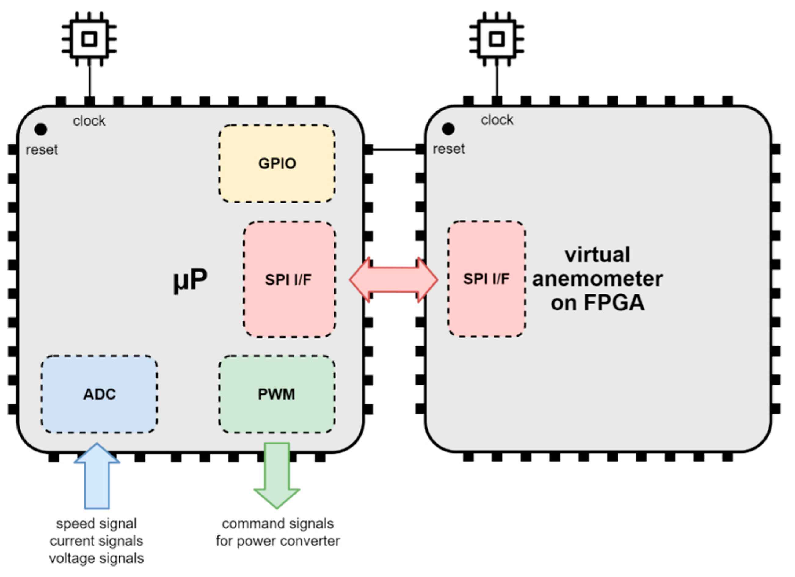
  • The interaction between the main processing platform and the virtual anemometer coprocessor is better described with the help of a new figure;
  • The reuse factor of VHDL components that exploit resource sharing has been explicitly stated;
  • The code of the chosen parallel sorting algorithm has been added;
  • The compatibility of the virtual anemometer FPGA design with application-specific integrated circuit (ASIC) and system-on-chip (SoC) implementations has been highlighted; in particular, it has been shown that even the low-end, commercial SoCs have an adequate number of resources to implement the virtual anemometer.
The paper is structured as follows. The wind turbine models that are learned by the GNG ANN are presented in Section 2. The details of the GNG ANN, including the steps of the training and recalling algorithms, are described in Section 3. Then, Section 4 describes several aspects of the FPGA implementation of the virtual anemometer. The experimental validation procedure and the results are presented in Section 5. Finally, some conclusions are drawn.

2. Models of Horizontal and Vertical Axis Wind Turbines

The behavior of the proposed virtual anemometer is independent from the type and rating of the wind turbine under hand; hence, it can work with both vertical-axis and horizontal-axis turbines. The GNG ANN is trained using the set of mechanical characteristics (power/torque versus angular speed) of the chosen wind turbine for varying wind speed, which fully describe the steady-state turbine behavior. In particular, they can be obtained fitting the equations of the following two models, starting from datasets acquired either through a few experimental tests or as a result of finite element method (FEM) simulations.

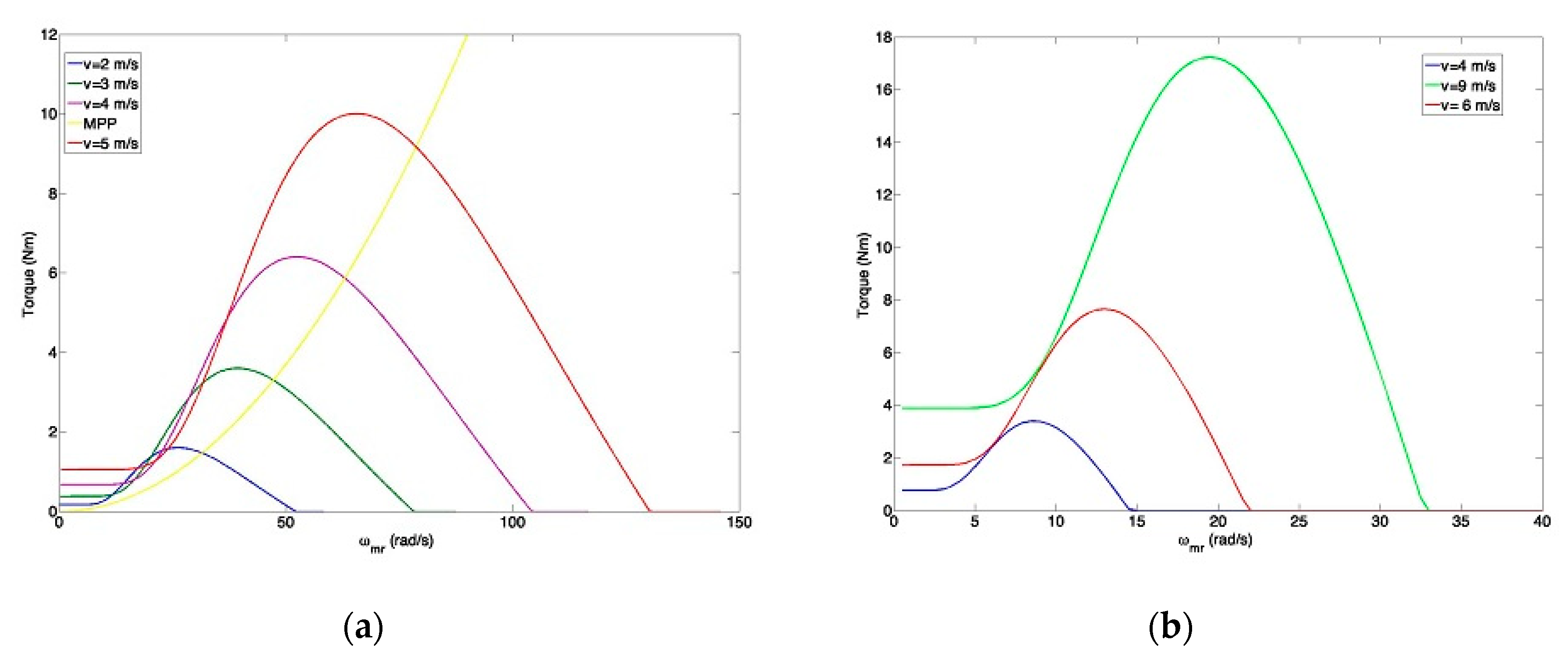
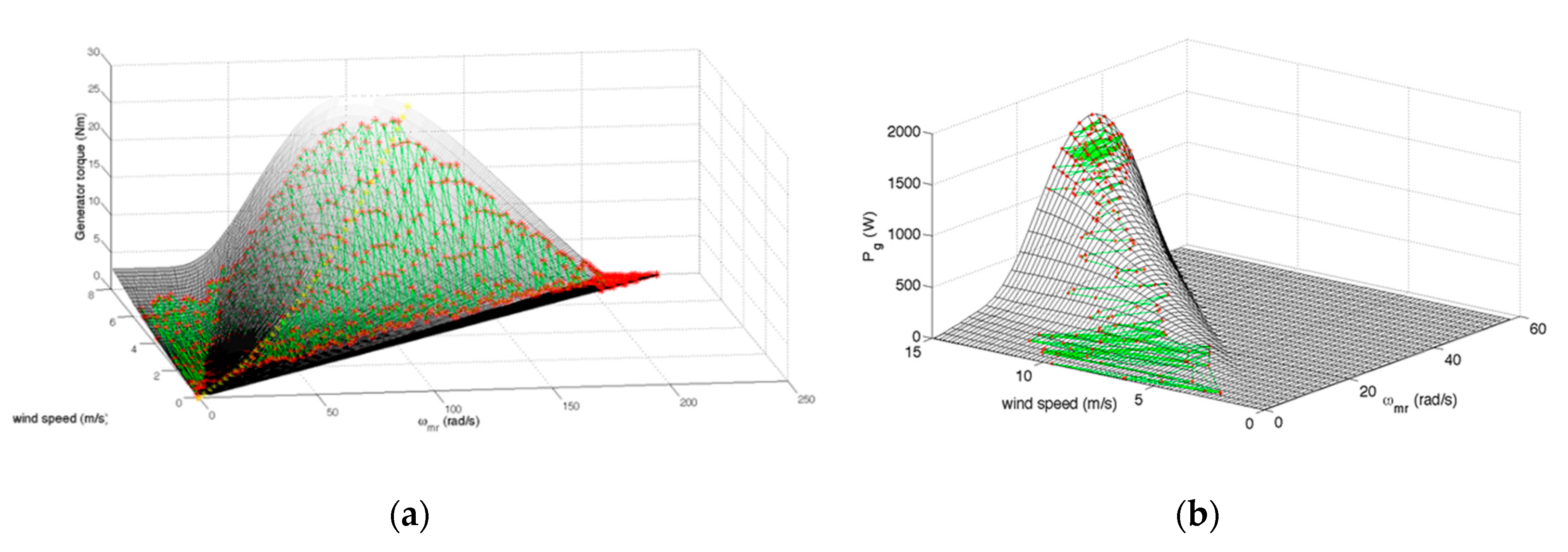
2.1. Horizontal Axis Wind Turbine

The power generated by a horizontal axis wind turbine (HAWT) can be written as [34]:
P m = C p ( λ , β ) ρ A 2 v 3 ,
where Pm is the mechanical power of the turbine in [W], Cp is the performance coefficient of the turbine, ρ is the air density in [kg/m3], A is the turbine swept area in [m2], v is the wind speed in [m/s], β is the blade pitch angle in [deg], and λ is the tip speed ratio defined as the ratio of the rotor blade tip to the speed of the wind:
λ = ω T R v .
In (2), ωT is the turbine angular speed, and R is the turbine radius. The performance coefficient is expressed by:
C P ( λ , β ) = c 1 ( c 2 λ i c 3 β c 4 ) e c 5 λ i + c 6 λ ,
with:
1 λ i = 1 λ + 0.08 β 0.035 β 3 + 1 ,
and the coefficients c 1 c 6 can be determined by fitting the mechanical characteristics of the wind turbine. Given the mechanical power, the torque produced by the turbine can be computed as:
T T = P m ω T = C T ( λ , β ) ρ π R 3 2 v 2 ,
where the torque coefficient of the turbine is defined as C T ( λ , β ) = C P ( λ , β ) / λ . Finally, it is worth recalling that both turbine speed and torque should be converted into the machine speed range by considering the gear ratio n:
ω T = ω T n = ω r m   and   T T = T T / n .

2.2. Vertical Axis Wind Turbine

The power generated by a vertical axis wind turbine (VAWT) can be written as follows:
P m = [ ( a 1 + a 2 v ω T ) e ( a 3 v ω T ) + a 4 ω T v ] v 3 .
Therefore, the turbine torque can be expressed as:
T T = [ ( a 1 + a 2 v ω T ) e ( a 3 v ω T ) + a 4 ω T v ] v 3 ω T .
The equations of the VAWT present a very similar structure to Equations (1)–(5), but they require the knowledge of only four coefficients; i.e., a 1 a 4 . As in the HAWT case, the parameters can be determined by fitting the mechanical characteristics of the wind turbine, either from experimental measurements or from the results of FEM simulations.

3. The GNG Artificial Neural Network
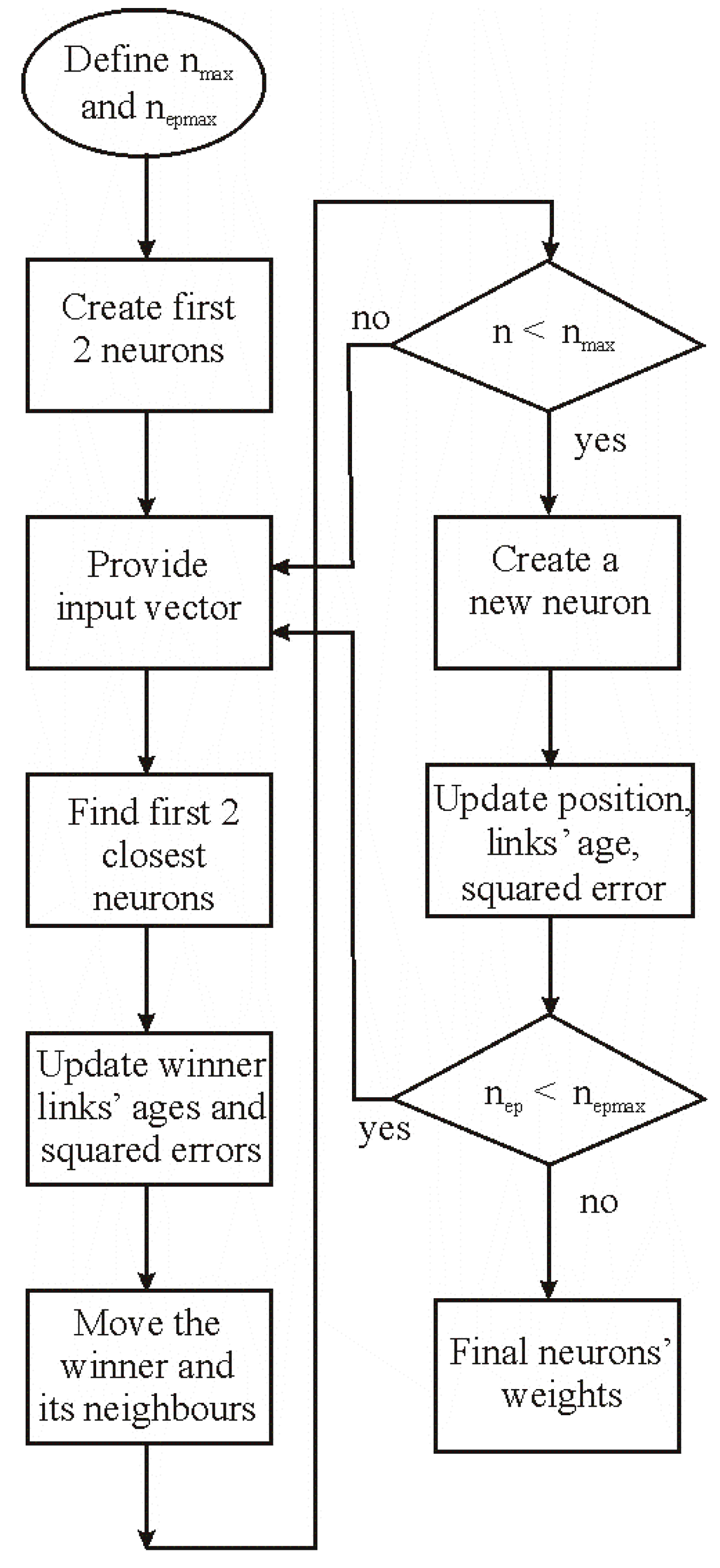
The growing neural gas (GNG) is a particular kind of self-supervised neural network. The basic principle of the GNG is to start with an initially small network with only two units (neurons) and progressively increase the number of units in a growing structure [30,35,36]. The maximum size of the network is chosen a priori by the user considering the nature of data and the dimensionality of the working space. The underlying idea is that a limited number of units (neurons) can properly represent a larger amount of data. To perform this task, the network of neurons must be initially trained. During the training phase, the network learns the data, and consequently, the final configuration of the network is determined; such a phase, which is the most demanding from the computational point of view, is performed offline on a standard PC. Once the network is trained, its online employment is performed by means of the so-called recalling phase. In this phase, the network is used to predict the system output starting from previously unseen input data. The recalling phase is usually performed online and runs on a suitably chosen hardware platform.
In the application under study, once the direct function of Section 2 that expresses the wind turbine model, i.e., P m = f ( v , ω m ) or T T = f ( v , ω m ) , is learned on the basis of the experimental data, the GNG can compute v e s t i m = f 1 ( P m , ω m ) or v e s t i m = f 1 ( T T , ω m ) online during the recalling phase. In this way, it is possible to estimate wind speed on the basis of the actual values of wind turbine speed and mechanical power/torque. In the following, the algorithms of training and recalling phases are described.

3.1. Training Phase

The complete algorithm for GNG training is summarized in the following steps:
  • Start with two neurons a and b with random weights wa and wb in ℜn;
  • Present an input signal ξ belonging to the training dataset;
  • Find the nearest neuron s1 and the second nearest neuron s2;
  • Increment the age of all edges emanating from s1;
  • Add the squared distance between the input signal and the nearest neuron in the input space to a local counter variable:
    Δ e r r o r ( s 1 ) = w s 1 ξ 2
  • Move s1 in its direct topological neighbors towards ξ by fractions εb and εn, respectively, of the total distance:
    { Δ w s 1 = ε b ( ξ w s 1 ) Δ w n = ε n ( ξ w n )
    for all direct neighbors n of s1;
  • If s1 and s2 are connected by an edge, set the age of this edge to zero; if such an edge does not exist, create it;
  • Remove edges with an age larger than amax; if this results in points with no emanating edges, remove them;
  • If the number of input data presented so far is an integer multiple of a parameter λ, create a new neuron as follows:
    • Determine the neuron q with the maximum accumulated error;
    • Insert a new neuron r halfway between q and its neighbor f, and remove the original edge between q and f;
    • Decrease the error variables of q and f multiplying them by a constant α; initialize the error variable of r with the new value of the error variable of q;
  • Decrease all error variables multiplying them by a constant d;
  • If a stopping criterion (e.g., net size or performance criterion) is not yet fulfilled, then go to step 2.
The flowchart of the training algorithm, which synthetizes the above-described procedure, is shown in Figure 1.

3.2. Recalling Phase

The recalling algorithm of the GNG is summarized as follows:
  • Present the input vector ξ i ;
  • Compute the K Euclidean distances Dk between the vector ξ i and the weights wi,k of the K neurons of the GNG;
  • Sort the Dk’s in ascending order and consider the corresponding first P neurons;
  • Compute the estimated output y by:
    y = 1 P   w i , k D k 1 P 1   D k .
It is worth noting that the GNG ANN works differently from other classic supervised neural networks like the MLP ANN trained by the back-propagation algorithm. In fact, the GNG ANN considers the neurons that are closer to the input data, and it computes the output as its weighted sum (Equation (9)). This way, the computational demand is reduced with respect to the MLP ANN, which requires the evaluation of several non-linear functions, called activation functions (one for each neuron). On the other hand, a GNG ANN usually requires a much higher number of neurons in comparison to an MLP ANN.

4. FPGA Implementation of the Virtual Anemometer

The virtual anemometer consists of a coprocessor in the form of a programmed FPGA that can be interfaced with the processing platform in which the control scheme of the WG is implemented, i.e., a µP, µC, or DSP. The interaction between the main processing platform and the coprocessor is summarized by the synopsis of Figure 2. As for the communication bus, SPI interface was chosen and implemented in the FPGA because of its high performance, wide diffusion, and availability as a hardware peripheral within several processing platforms. In the following, a µP-based control system is assumed with no loss of generality; in fact, if µCs or DSPs are used for WG control, they can exchange data with the virtual anemometer in the same way because they have at least one SPI interface available and several general purpose input/output (GPIO) pins.
The μP that executes the control system of the WG periodically sends the values of the electrical machine’s angular speed and torque (or power) to the virtual anemometer using the SPI interface. These are two variables that are already processed in the control system. Then, the virtual anemometer performs its computation and returns the estimated value of wind speed to the μP, which exploits the virtual measurement to perform model-based MPPT of the WG and to compute the command signals for the related power electronic converter accordingly.
In particular, the angular speed is measured by an incremental encoder; the torque, instead, can be estimated starting from the current signals by suitable torque models (based on flux observers/estimators) that can be embedded into the control algorithm of the WG. If needed, the power can be computed multiplying angular speed by torque.
The virtual anemometer is programmed just once using the neuron weights that result from the training phase of the GNG ANN, in which the whole set of wind turbine characteristics is learned. Because of this, the virtual anemometer works accurately in the whole wind speed range of the wind turbine. It is also worth highlighting that the virtual anemometer is equivalent to a real anemometer, which is a sensor that performs instantaneous measurements of wind speed. As such, it is not able to make either short-term or long-term predictions of wind load. If this feature is needed, a forecasting algorithm should be used instead of the virtual anemometer.
To obtain a well optimized design, the VHDL code describing the hardware design of the virtual anemometer has been manually written. The synopsis of the FPGA design is presented in Figure 3, where the internal connections of reset and clock lines have been omitted for the sake of simplicity. The details of the SPI communication interface and the GNG ANN implementation are described in the following subsections.

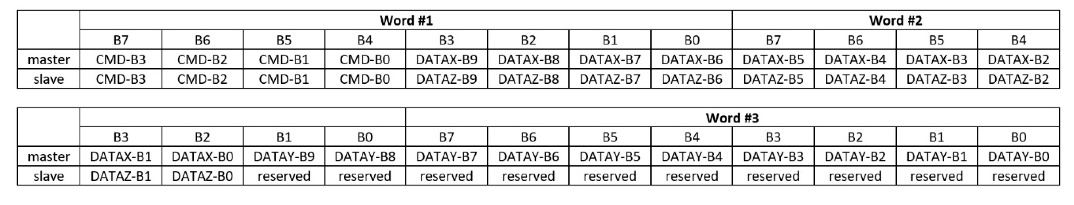
4.1. SPI Communication Interface and Protocol

The communication between the microprocessor and the coprocessor exploits an SPI bus with a 12 MHz clock. Data are exchanged through transactions involving three consecutive 8-bit words.
The packet structure for master (microprocessor) and slave (FPGA) communication on SPI bus is shown in Figure 4. Each command (CMD) is issued by setting the first half word of the packet. If the master starts sending CMD = 0001, then the following data are the 20 bits of the x and y inputs for the GNG ANN; if the slave starts answering with CMD = 0001, then the following data are the 10 bits of the z output of the GNG ANN. Other CMD values are currently reserved for future uses; e.g., to update ANN weights online.
A finite state machine (FSM) is used as a supervisor that coordinates the data exchange between the SPI module and the GNG ANN, also providing error detection.

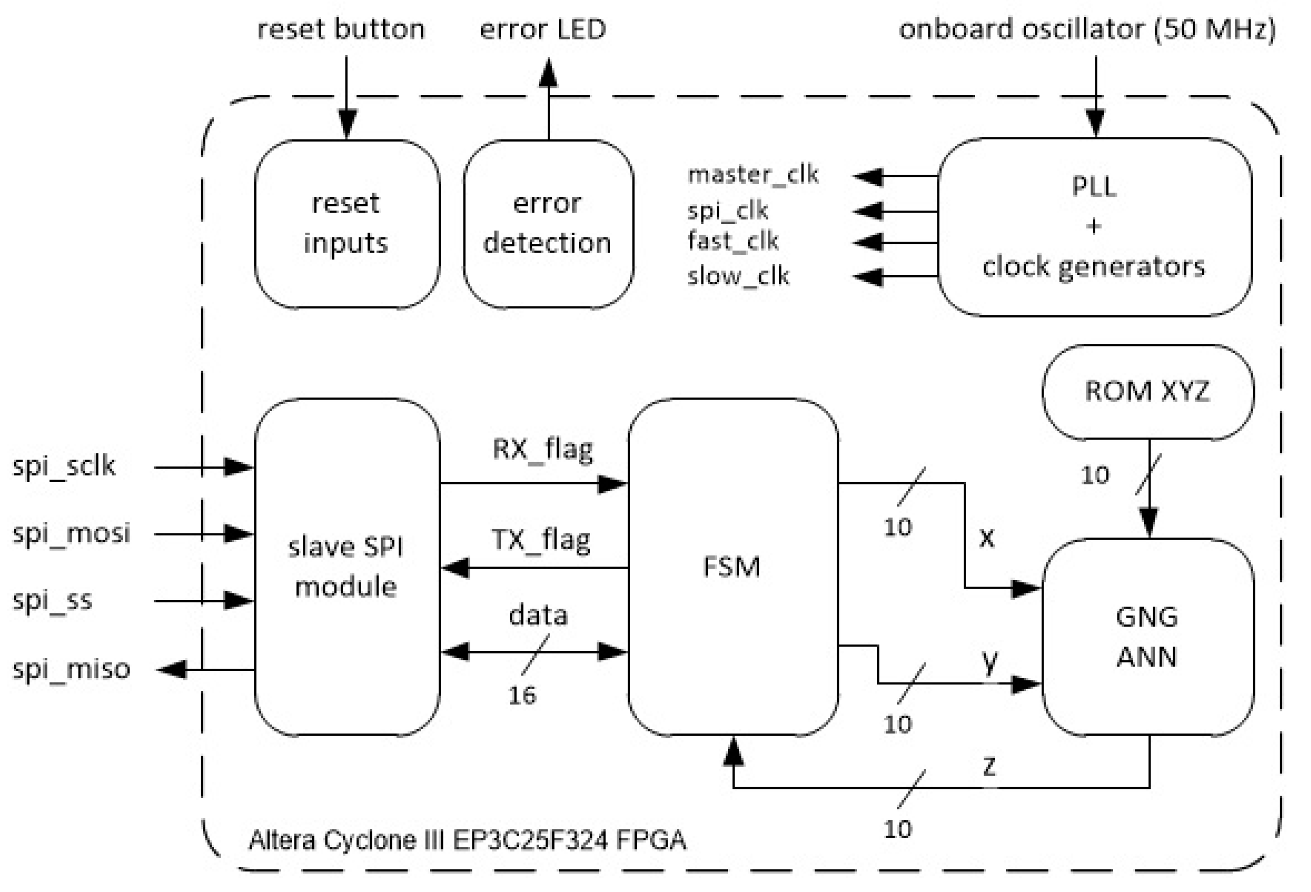
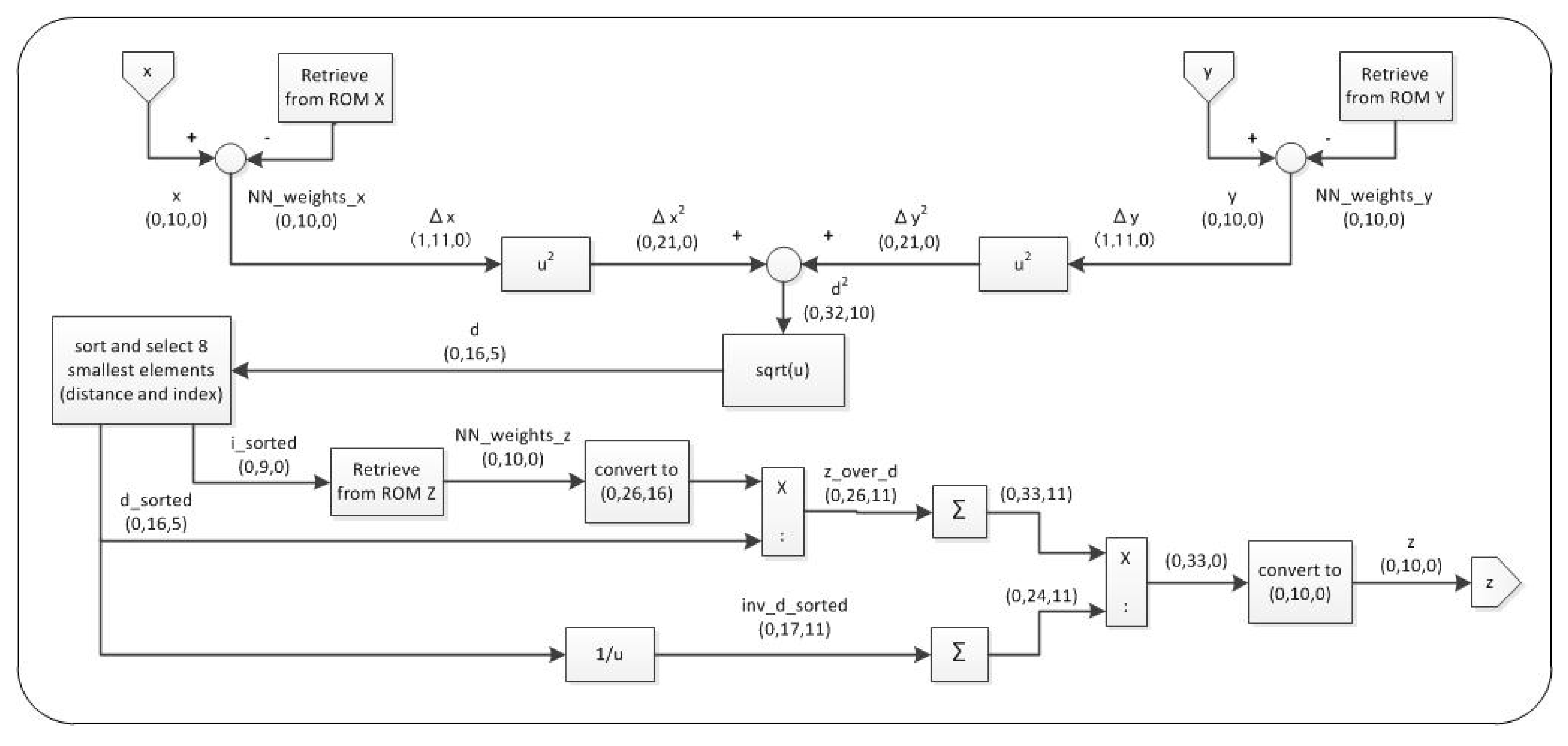
4.2. GNG ANN Implementation

The GNG ANN is supposed not to vary its structure (neuron number and weights) dynamically online. Thus, the training algorithm, in which the ANN learns the relationship y = f ( x , z ) using the provided training dataset, can be executed offline just once on a standard PC obtaining the weights of the ANN. Such weights are the x-y-z coordinates of each neuron and must be stored in the ROM XYZ implemented in the FPGA during the programming operation. The recalling algorithm of the GNG ANN is then the only algorithm implemented and executed online on the FPGA to compute the inverse function z = f 1 ( x , y ) starting from the data transmitted by the microprocessor.
The block diagram describing the implementation of the recalling algorithm according to Section 3.2 is sketched in Figure 5. The goal pursued was to implement such an algorithm achieving a suitable compromise between computation speed and resource utilization, so as to use a low-range, low-cost FPGA such as the Altera Cyclone III EP3C25F324 [37]. It is worth noting that wrong technical choices could negatively affect system performance, either reducing the estimation accuracy or hindering the implementation on the chosen programmable platform. Hence, 512 neurons have been considered; i.e., more than enough to obtain the required accuracy in wind speed estimation [13]. Furthermore, the following other technical choices have been made:
  • The inputs/outputs of the ANN are 10-bit integers as the data width of most ADCs commonly used within control systems;
  • The weights of the ANN are also 10-bit integers, and they are stored in a ROM that is implemented using some of the dedicated memory blocks inside the FPGA chip;
  • Hardware multipliers are used for computing blocks Δx2 and Δy2 of Figure 5;
  • Fixed point arithmetic is used; the related precision varies from 10 bit to 32 bit; in particular, Figure 5 indicates the used datatype as a triplet (s,b,f), where s = sign bit, b = total number of bits, f = number of fractional bits;
  • The final weighted sum is computed considering the eight neurons closest to the input data;
  • True parallel implementation was chosen for blocks u−1, u1/u2, sqrt(u);
  • Resource sharing is enforced for blocks u2 and for the sorting component with a reuse factor equal to 32;
  • For this latter component a fast, parallel sorting algorithm, i.e., bitonic sort [38], has been chosen; this algorithm was implemented to select the eight smallest values among 16 input numbers; hence, the obtained VHDL component processes the distances from the input point to all neurons in blocks of 16 on several consecutive clock cycles; the bitonic sort algorithm, written as Matlab code, is shown in Algorithm 1.
To obtain a modular and scalable design, several parameters (clock frequencies, neuron number, input data width, etc.) were implemented as VHDL generics. Therefore, changing such values does not break the design operation after recompilation. This is an interesting feature that simplifies further improvements of the virtual sensor and the use of the GNG ANN in other contexts.
The required frequency for the external oscillator is 50 MHz, and Table 1 summarizes the resources used within the Altera EP3C25F324C8 FPGA. The maximum clock frequency for the implemented GNG ANN is 7 MHz. Considering this value, the SPI clock frequency, the number of bits to transmit and the delays required by the SPI protocol, the maximum frequency of data exchange between the FPGA and the microprocessor is 100 kHz. Hence, the data rate of the virtual anemometer is considerably faster than the execution time of even the most demanding current loop of any WG control system. In other words, the use of the virtual anemometer does not worsen the performance of the WG control system.
Finally, it is worth noting that there are two alternatives to produce the proposed virtual anemometer. If mass production of the device is needed, the design can be implemented as an application-specific integrated circuit (ASIC) on the basis of the same VHDL code of the FPGA implementation. Otherwise, a system-on-chip (SoC) could be used to implement both the microprocessor and the FPGA coprocessor of Figure 2 on the same device. This choice would reduce system cost, weight, volume, and power consumption. Being written in standard VHDL, the design of the virtual anemometer is compatible with the programmable logic of every SoC, provided that enough hardware resources are available. Only a recompilation for the chosen target would be needed. For example, the Xilinx Zynq SoC could be used [39]. This device, even in the less performing version (Zynq Z-7007S), encompasses a powerful ARM Cortex-A9 microprocessor and Artix 7 programmable logic with a sufficient number of hardware resources, as shown in Table 1.
Algorithm 1. Matlab code of Bitonic Sort algorithm.
% this function implements bitonic sort algorithm
% in ascending order for 16 input elements
function outVec = bitonicSorter(inVec)
    outVec = bitonicSort16(inVec);
end
function out = bitonicSort16(in)
    out(1:8) = bitonicSort8(in(1:8), true);
    out(9:16) = bitonicSort8(in(9:16), false);
    out = bitonicMerge16(out, true);
end
function out = bitonicSort8(in, direction)
    out(1:4) = bitonicSort4(in(1:4), true);
    out(5:8) = bitonicSort4(in(5:8), false);
    out = bitonicMerge8(out, direction);
end
function out = bitonicSort4(in, direction)
    out(1:2) = bitonicSort2(in(1:2), true);
    out(3:4) = bitonicSort2(in(3:4), false);
    out = bitonicMerge4(out, direction);
end
function out = bitonicSort2(in, direction)
  out = bitonicMerge2(in, direction);
end
function out = bitonicMerge16(in, direction)
    for i = 1:8
        tmp = compare([in(i); in(i + 8)], direction);
        out(i) = tmp(1);
        out(i+8) = tmp(2);
    end
    out(1:8) = bitonicMerge8(out(1:8), direction);
    out(9:16) = bitonicMerge8(out(9:16), direction);
end
function out = bitonicMerge8(in, direction)
    for i = 1:4
        tmp = compare([in(i); in(i + 4)], direction);
        out(i) = tmp(1);
        out(i+4) = tmp(2);
    end
    out(1:4) = bitonicMerge4(out(1:4), direction);
    out(5:8) = bitonicMerge4(out(5:8), direction);
end
function out = bitonicMerge4(in, direction)
    for i = 1:2
        tmp = compare([in(i); in(i + 2)], direction);
        out(i) = tmp(1);
        out(i+2) = tmp(2);
    end
    out(1:2) = bitonicMerge2(out(1:2), direction);
    out(3:4) = bitonicMerge2(out(3:4), direction);
end
function out = bitonicMerge2(in, direction)
    out = compare([in(1); in(2)], direction);
end
function out = compare(in, direction)
    if direction == (in(1) > in(2))
        out = [in(2); in(1)];
    else
        out = in;
    end
end

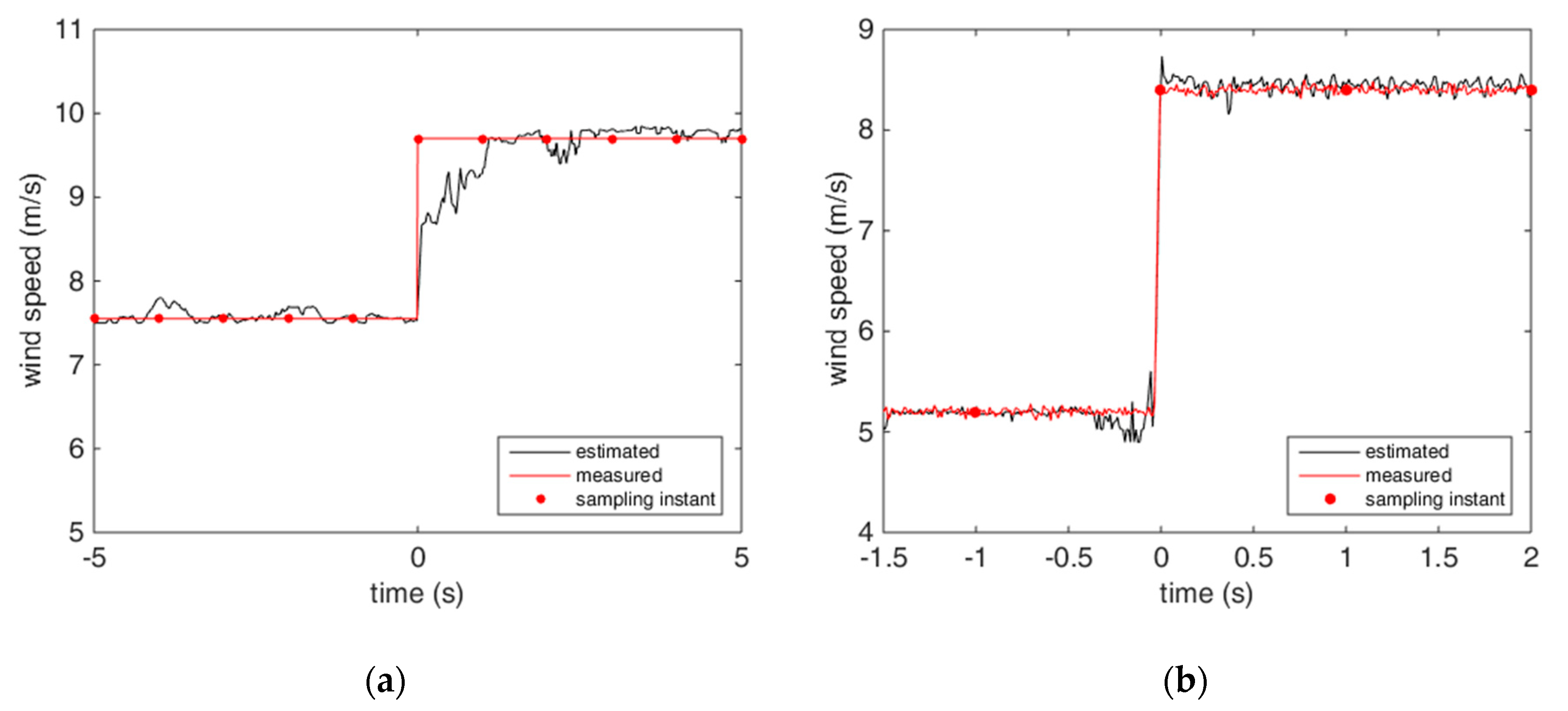
5. Experimental Validation

A standard PC equipped with a Silicon Labs CP2130 USB-to-SPI Protocol Converter has been used to communicate with the FPGA board. A specific application has been written to exchange data using the CP2130 C/C++ libraries in the same way as the µP (or µC or DSP) would do.
The virtual anemometer has been validated using two sets of data (wind speed, angular speed, and power/torque) that have been previously acquired experimentally during the operation of two WGs: a 5.5 kW horizontal axis wind turbine (HAWT) and a 1 kW vertical axis (Darrieus type) wind turbine (VAWT). As for wind speed measurement, the first turbine was equipped with a Windmeter cup anemometer by Soluzione Solare with an RS485 digital output and 1 Hz output sampling rate. On the other hand, the VAWT was equipped with a DeltaOhm HD 2003 ultrasonic anemometer with analog output and 1 Hz output sampling rate. The model parameters of the chosen HAWT/VAWT are shown in Table 2 and Table 3, respectively. Figure 6a,b shows the torque versus speed characteristics for varying wind speed of the HAWT and VAWT under study, respectively.
For each scenario, the GNG ANN has been set-up and trained offline in Matlab environment using 70% of the related dataset, obtaining a set of weights that has been stored into the ROM of the virtual anemometer. Such training data are shown in Figure 7a,b in gray and represent the characteristic surfaces (in terms of turbine torque/power, wind speed, and angular speed) of the HAWT and VAWT under study. Furthermore, Figure 7a,b also show the neurons of the trained GNG and their connections. As the figures show, the neurons lie on the characteristic surfaces.
Since the GNG is a static ANN, the correct operation of the FPGA-based virtual anemometer in each scenario has been verified with reference to its static behavior by comparing the estimated and measured wind speed profiles, starting from the test dataset (i.e., the remaining 30% of each original dataset). The wind speed profile has been estimated by presenting the GNG ANN with couples of input values (angular speed and power/torque) taken from the test dataset, sequentially. Therefore, each estimated wind speed value was compared with the measured wind speed value that corresponded to the angular speed and power/torque used as input for the estimation. In particular, torque and angular speed profiles have been considered in the first scenario, whereas power and angular speed profiles have been chosen for the other one. These two different choices depend on the different electrical signals available in HAWTs and VAWTs, since they exploit different topologies of power converters and related control systems.
For the sake of clarity, the comparison between estimated and measured wind speed profiles is presented in Figure 8a,b considering a sample interval for each scenario. As the figures show, the estimated wind speed tracks the measured wind speed at steady-state. This happens throughout the entire test dataset. Being this condition verified, each steady-state triplet (wind speed, angular speed, torque/power) is coherent and represents a point that belongs to the surface of mechanical characteristics of the wind turbine, validating the estimation process and the static operation of the virtual anemometer.
It is worth remarking that, despite the use of a static ANN, the virtual anemometer exhibits an estimation transient because, although the real wind speed stays constant after its rising edge, its input variables are affected by the mechanical dynamics of the wind turbine, which are slower for the HAWT (Figure 8a) than for the VAWT (Figure 8b).
As for the dynamic behavior of the proposed virtual anemometer, the following considerations hold. The variation of wind turbine torque/power in response to a wind speed variation is nearly instantaneous, whereas the angular speed varies according to the mechanical dynamics of the wind turbine. The virtual anemometer has high bandwidth, so its output variation is instantaneous as the torque/power variation (t = 0). However, the estimation lag depends on the settlement of angular speed. On the other hand, the real anemometer has a low sampling rate, so it can update its output up to one sampling time after the real wind variation. For example, referring to Figure 8a, the output of the real anemometer (red curve) could have been updated up to 1 second after the output variation of the virtual anemometer (t = 0), exhibiting almost the same lag. Instead, referring to Figure 8b, the output of the virtual anemometer does not exhibit an appreciable lag because of the lower mechanical inertia of the VAWT; thus, it meets or exceeds the performance of the real anemometer, whose lag can be up to 1 second.
In any case, the presence of a short lag in the output of the real/virtual anemometer is not a problem. In fact, the tracking time of a model-based MPPT that exploits such anemometers is significantly faster than that of any iterative MPPT algorithm, which must be much slower than the mechanical dynamics of the wind turbine to wait for the settlement after each perturbation.
In other words, the proposed virtual anemometer can be an effective and cheaper alternative to a real anemometer for performing model-based MPPT.

6. Conclusions

A high-performance implementation of an FPGA-based virtual anemometer that allows model-based maximum power point tracking (MPPT) of wind generators (WGs) has been presented. It was based on a growing neural gas artificial neural network (GNG ANN) that was implemented on a low-cost FPGA platform. As an alternative, it could be implemented as an ASIC or on the programmable logic of a system-on-chip (SoC) by simply recompiling for the different target.
The best compromise between resource occupation and speed was achieved through suitable hardware optimizations. The proposed virtual anemometer was conceived for embedded applications, unlike other virtual sensors proposed in the literature. Since it is able to exchange data up to a 100 kHz rate, it is suitable for high-performance model-based MPPT of WGs.
The proposed system has been validated on a commercial FPGA, taking advantage of two sets of wind turbine data (wind speed, angular speed, and power/torque) that have been previously acquired experimentally, and discussing both the static and dynamic behavior.

Author Contributions

Conceptualization and methodology, M.P., M.L., and G.L.T.; software development, G.L.T., M.L., and A.A.; validation, G.L.T., M.L., M.C.D.P., M.P., and A.A.; writing—review and editing, G.L.T., M.L., M.C.D.P., M.P., and A.A. All authors have read and agreed to the published version of the manuscript.

Funding

This research received no external funding.

Conflicts of Interest

The authors declare no conflict of interest.

References

  1. Reisi, A.R.; Moradi, M.H.; Jamasb, S. Classification and comparison of maximum power point tracking techniques for photovoltaic system: A review. Renew. Sustain. Energy Rev. 2013, 19, 433–443. [Google Scholar] [CrossRef]
  2. Zhou, M.; Bao, G.; Gong, Y. Maximum Power Point Tracking Strategy for Direct Driven PMSG. In Proceedings of the Asia-Pacific Power and Energy Engineering Conference (APPEEC), Wuhan, China, 25–28 March 2011; pp. 1–4. [Google Scholar]
  3. Hsieh, G.C.; Hsieh, H.I.; Tsai, C.Y.; Wang, C.H. Photovoltaic Power-Increment-Aided Incremental-Conductance MPPT with Two-Phased Tracking. IEEE Trans. Power Electron. 2013, 28, 2895–2911. [Google Scholar] [CrossRef]
  4. Syahputra, R.; Soesanti, I. Performance Improvement for Small-Scale Wind Turbine System Based on Maximum Power Point Tracking Control. Energies 2019, 12, 3938. [Google Scholar] [CrossRef] [Green Version]
  5. Abo-Khalil, A.G.; Lee, D.-C.; Seok, J.-K. Variable speed wind power generation system based on fuzzy logic control for maximum output power tracking. In Proceedings of the 35th Annual IEEE Power Electronics Specialists Conference (PESC 04), Aachen, Germany, 20–25 June 2004. [Google Scholar]
  6. Leidhold, R.; Garcia, G.; Valla, M.I. Maximum efficiency control for variable speed wind driven generators with speed and power limits. In Proceedings of the 28th Annual International Conference of the IEEE Industrial Electronics Society (IECON), Sevilla, Spain, 5–8 November 2002; pp. 57–162. [Google Scholar]
  7. Chedid, R.; Mrad, F.; Basma, M. Intelligent control of a class of wind energy conversion systems. IEEE Trans. Energy Convers. 1999, 14, 1597–1604. [Google Scholar] [CrossRef]
  8. Thongam, J.S.; Bouchard, P.; Ezzaidi, H.; Ouhrouche, M. Artificial neural network-based maximum power point tracking control for variable speed wind energy conversion systems. In Proceedings of the 2009 IEEE Control Applications, (CCA) & Intelligent Control, (ISIC), St. Petersburg, Russia, 8–10 July 2009; pp. 1667–1671. [Google Scholar]
  9. Gwang, H.; Seung, R.H.; Lee, K.B. An Improved Maximum Power Point Tracking Method for Wind Power Systems. Energies 2012, 5, 1339–1354. [Google Scholar] [CrossRef] [Green Version]
  10. Zhang, Y.; Zhang, L.; Liu, Y. Implementation of Maximum Power Point Tracking Based on Variable Speed Forecasting for Wind Energy Systems. Processes 2019, 7, 158. [Google Scholar] [CrossRef] [Green Version]
  11. Thongam, J.S.; Bouchard, P.; Beguenane, R.; Fofana, I. Neural network based wind speed sensorless MPPT controller for variable speed wind energy conversion systems. In Proceedings of the 2010 IEEE Electric Power and Energy Conference (EPEC), Halifax, NS, Canada, 25–27 August 2010; pp. 1–6. [Google Scholar]
  12. Cirrincione, M.; Pucci, M.; Vitale, G. Growing Neural Gas (GNG) based Maximum Power Point Tracking for High Performance Wind Generator System with Induction Machine. IEEE Trans. Ind. Appl. 2011, 47, 861–872. [Google Scholar] [CrossRef]
  13. Pucci, M.; Cirrincione, M. Neural MPPT Control of Wind Generators with Induction Machines Without Speed Sensors. IEEE Trans. Ind. Electron. 2011, 58, 37–47. [Google Scholar] [CrossRef]
  14. Mesemanolis, A.; Mademlis, C. A Neural Network based MPPT controller for variable speed Wind Energy Conversion Systems. In Proceedings of the 8th Mediterranean Conference on Power Generation, Transmission, Distribution and Energy Conversion (MEDPOWER 2012), Cagliari, Italy, 1–3 October 2012; pp. 1–6. [Google Scholar]
  15. Vitale, G.; Pucci, M.; Luna, M. Metodo e Relativo Sistema Per la Conversione di Energia Meccanica, Proveniente da un Generatore Comandato da una Turbina, in Energia Elettrica. IT Patent No. 0,001,417,881, 4 September 2015. [Google Scholar]
  16. Vitale, G.; Pucci, M.; Luna, M. Method and Relevant System for Converting Mechanical Energy from a Generator Actuated by a Turbine into Electric Energy. U.S. Patent No. 9,856,857 B2, 2 January 2018. [Google Scholar]
  17. Di Piazza, M.C.; Luna, M.; Pucci, M.; Vitale, G. PV-based Li-ion battery charger with neural MPPT for autonomous sea vehicles. In Proceedings of the 39th Annual Conference of the IEEE Industrial Electronics Society (IECON), Vienna, Austria, 10–13 November 2013; pp. 7267–7273. [Google Scholar]
  18. Liu, L.; Kuo, S.M.; Zhou, M. Virtual sensing techniques and their applications. In Proceedings of the 2009 International Conference on Networking, Sensing and Control (ICNSC), Okayama, Japan, 26–29 March 2009; pp. 31–36. [Google Scholar]
  19. Chatterjee, A.; Keyhani, A. Neural Network Estimation of Microgrid Maximum Solar Power. IEEE Trans. Smart Grid 2012, 3, 1860–1866. [Google Scholar] [CrossRef]
  20. Ceylan, I.; Erkaymaz, O.; Gedik, E.; Gürel, A.E. The prediction of photovoltaic module temperature with artificial neural networks. Case Stud. Therm. Eng. 2014, 3, 11–20. [Google Scholar] [CrossRef] [Green Version]
  21. Ferreira, P.M.; Gomes, J.M.; Martins, I.A.C.; Ruano, A.E. A Neural Network Based Intelligent Predictive Sensor for Cloudiness, Solar Radiation and Air Temperature. Sensors 2012, 12, 15750–15777. [Google Scholar] [CrossRef] [PubMed]
  22. Karatepe, E.; Hiyama, T. Artificial neural network-polar coordinated fuzzy controller based maximum power point tracking control under partially shaded conditions. IET Renew. Power Gener. 2009, 3, 239–253. [Google Scholar]
  23. Mancilla-David, F.; Riganti Fulginei, F.; Laudani, A.; Salvini, A. A Neural Network-Based Low-Cost Solar Irradiance Sensor. IEEE Trans. Instrum. Meas. 2014, 63, 583–591. [Google Scholar] [CrossRef]
  24. Oliveri, A.; Cassottana, L.; Laudani, A.; Fulginei, F.R.; Lozito, G.M.; Salvini, A.; Storace, M. Two FPGA-Oriented High-Speed Irradiance Virtual Sensors for Photovoltaic Plants. IEEE Trans. Ind. Informat. 2017, 13, 157–165. [Google Scholar] [CrossRef]
  25. Hwang, Y.; Minami, Y.; Ishikawa, M. Virtual Torque Sensor for Low-Cost RC Servo Motors Based on Dynamic System Identification Utilizing Parametric Constraints. Sensors 2018, 18, 3856. [Google Scholar] [CrossRef] [PubMed] [Green Version]
  26. Guzmán, C.; Carrera, J.; Durán, H.; Berumen, J.; Ortiz, A.; Guirette, O.; Arroyo, A.; Brizuela, J.; Gómez, F.; Blanco, A.; et al. Implementation of Virtual Sensors for Monitoring Temperature in Greenhouses Using CFD and Control. Sensors 2018, 19, 60. [Google Scholar] [CrossRef] [PubMed] [Green Version]
  27. Cotton, N.J.; Wilamowski, B.M.; Dundar, G. A Neural Network Implementation on an Inexpensive Eight Bit Microcontroller. In Proceedings of the 2008 International Conference on Intelligent Engineering Systems, Miami, FL, USA, 25–29 February 2008; pp. 109–114. [Google Scholar]
  28. Yang, Y.R. A neural network controller for maximum power point tracking with 8-bit microcontroller. In Proceedings of the 2011 6th IEEE Conference on Industrial Electronics and Applications, Beijing, China, 21–23 June 2011; pp. 919–924. [Google Scholar]
  29. Kashif, S.A.R.; Saqib, M.A.; Zia, S.; Kaleem, A. Implementation of neural network based Space Vector Pulse Width Modulation inverter-induction motor drive system. In Proceedings of the 2009 3rd International Conference on Electrical Engineering (ICEE), Lahore, Pakistan, 9–11 April 2009; pp. 1–6. [Google Scholar]
  30. Fratta, A.; Griffero, G.; Nieddu, S. Comparative analysis among DSP and FPGA-based control capabilities in PWM power converters. In Proceedings of the 30th Annual Conference of the IEEE Industrial Electronics Society (IECON), Busan, Korea, 2–6 November 2004; pp. 257–262. [Google Scholar]
  31. Economou, G.P.K.; Mariatos, E.P.; Economopoulos, N.M.; Lymberopoulos, D.; Goutis, C.E. FPGA implementation of artificial neural networks: An application on medical expert systems. In Proceedings of the 4th International Conference on Microelectronics for Neural Networks and Fuzzy Systems, Turin, Italy, 26–28 September 1994; pp. 287–293. [Google Scholar]
  32. Fritzke, B. A Growing Neural Gas Network Learns Topologies, Advances in Neural Information Processing Systems 7; MIT Press: Cambridge, UK, 1995. [Google Scholar]
  33. Accetta, A.; Di Piazza, M.C.; Tona, G.L.; Luna, M.; Pucci, M. A high-performance FPGA-based virtual anemometer for MPPT of wind energy conversion systems. In Proceedings of the 2017 IEEE 26th International Symposium on Industrial Electronics (ISIE), Edinburgh, UK, 19–21 June 2017; pp. 926–933. [Google Scholar]
  34. Freris, L.L. Wind Energy Conversion System; Prentice Hall: New York, NY, USA, 1990. [Google Scholar]
  35. Fritzke, B. Growing Cell Structures—A self-organizing network for unsupervised and supervised learning. Neural Netw. 1994, 7, 1441–1460. [Google Scholar] [CrossRef]
  36. Fritzke, B. Incremental Learning of Linear Local Mappings. In Proceedings of the International Conference on Artificial Neural Networks (ICANN), Paris, France, 9–13 October 1995; pp. 217–222. [Google Scholar]
  37. Altera Cyclone III Device Handbook Volume 1. Available online: https://www.intel.com/content/dam/www/programmable/us/en/pdfs/literature/hb/cyc3/cyclone3_handbook.pdf (accessed on 30 October 2019).
  38. Batcher, K.E. Sorting Networks and their Applications. In Proceedings of the AFIPS Spring Joint Computer Conference, Atlantic City, NJ, USA, 30 April–2 May 1968; Volume 32, pp. 307–314. [Google Scholar]
  39. Zynq-7000 SoC Data Sheet: Overview. Available online: https://www.xilinx.com/support/documentation/data_sheets/ds190-Zynq-7000-Overview.pdf (accessed on 30 October 2019).
Figure 1. Flowchart describing the training algorithm of the Growing Neural Gas Artificial Neural Network.
Electronics 09 00083 g001
Figure 2. Synopsis of the interaction between the main microprocessor and the coprocessor.
Electronics 09 00083 g002
Figure 3. Block scheme of the virtual anemometer’s field programmable gate array (FPGA) implementation.
Electronics 09 00083 g003
Figure 4. Packet structure for serial peripheral interface (SPI) bus communication.
Electronics 09 00083 g004
Figure 5. Synopsis of the recalling algorithm implemented on FPGA.
Electronics 09 00083 g005
Figure 6. Torque versus speed characteristics for several wind speed values: (a) 5.5 kW horizontal axis wind turbine (HAWT) (locus of the MPPs in yellow); (b) 1 kW vertical axis wind turbine (VAWT).
Electronics 09 00083 g006
Figure 7. Neurons (red) and neuron connections (green) shown on the characteristic surface of turbine (gray): (a) torque versus wind speed versus angular speed for 5.5 kW HAWT; (b) power versus wind speed versus angular speed for 1 kW VAWT.
Electronics 09 00083 g007
Figure 8. Estimated and measured wind speed profiles: (a) 5.5 kW HAWT; (b) 1 kW VAWT. Red dots highlight the sampling instants of the real anemometer.
Electronics 09 00083 g008
Table 1. Comparison of requested and available resources.
Resource CountUsed by the Proposed DesignAvailable on Altera Cyclone III EP3C25F324Available on Xilinx Zynq Z-7007S
Logic elements/Prog. logic cells22,14824,62423,552
Registers/Flip-Flops226524,62428,800
Memory bits/Block RAM6528608,2561,887,436
Embedded multipliers/DSP slices3213266
Table 2. Parameters of the considered horizontal axis wind turbine.
ParameterValue
R [m]2.50
λopt7
Cpmax0.45
n4.86
Generator rated power [kW]5.5
Generator rated speed [rpm] 1500
Model coefficientsc1 = 0.5176, c2 = 116,
c3 = 0.4, c4 = 5,
c5 = 21, c6 = 0.0068
Table 3. Parameters of the considered vertical axis wind turbine.
ParameterValue
R [m]0.75
λopt2
Cpmax0.15
n1
Generator rated power [kW]1.0
Generator rated speed [rpm]415
Model coefficientsa1 = −25.6815,
a2 = 87.6095,
a3 = 8.0646,
a4 = 0.048076

