Fuel Cell Hybrid Model for Predicting Hydrogen Inflow through Energy Demand

 ,
,  ,
,  ,
,  and
and
Abstract
1. Introduction
2. Case Study
2.1. Test Bench
2.2. Power System
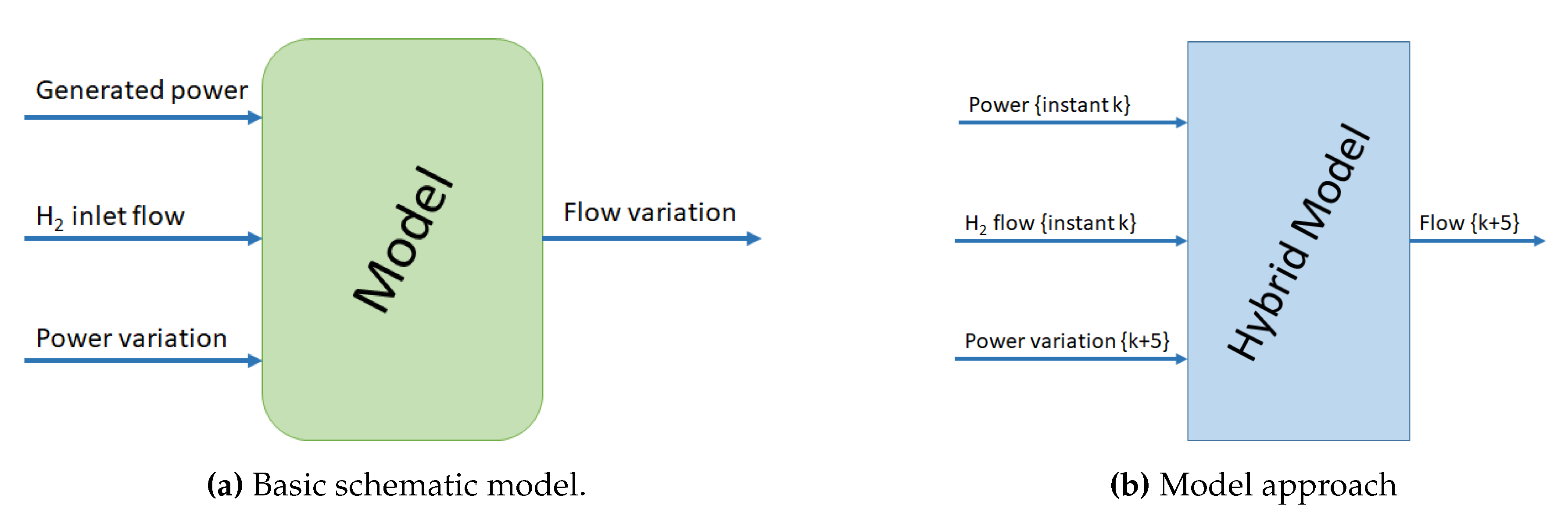
3. Model Approach
3.1. K-Means Algorithm
3.2. Artificial Neural Networks
3.3. Polynomial Regression
3.4. Data Processing
4. Results
4.1. Clustering Results
4.2. Modeling Results
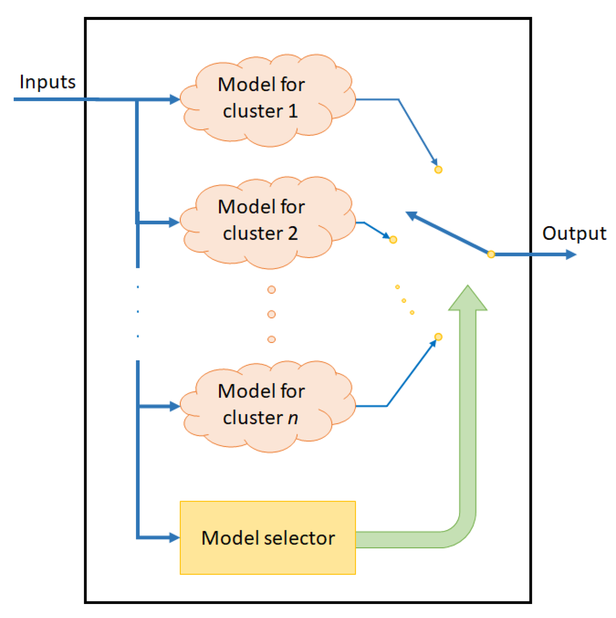
4.3. Hybrid Topology Selection
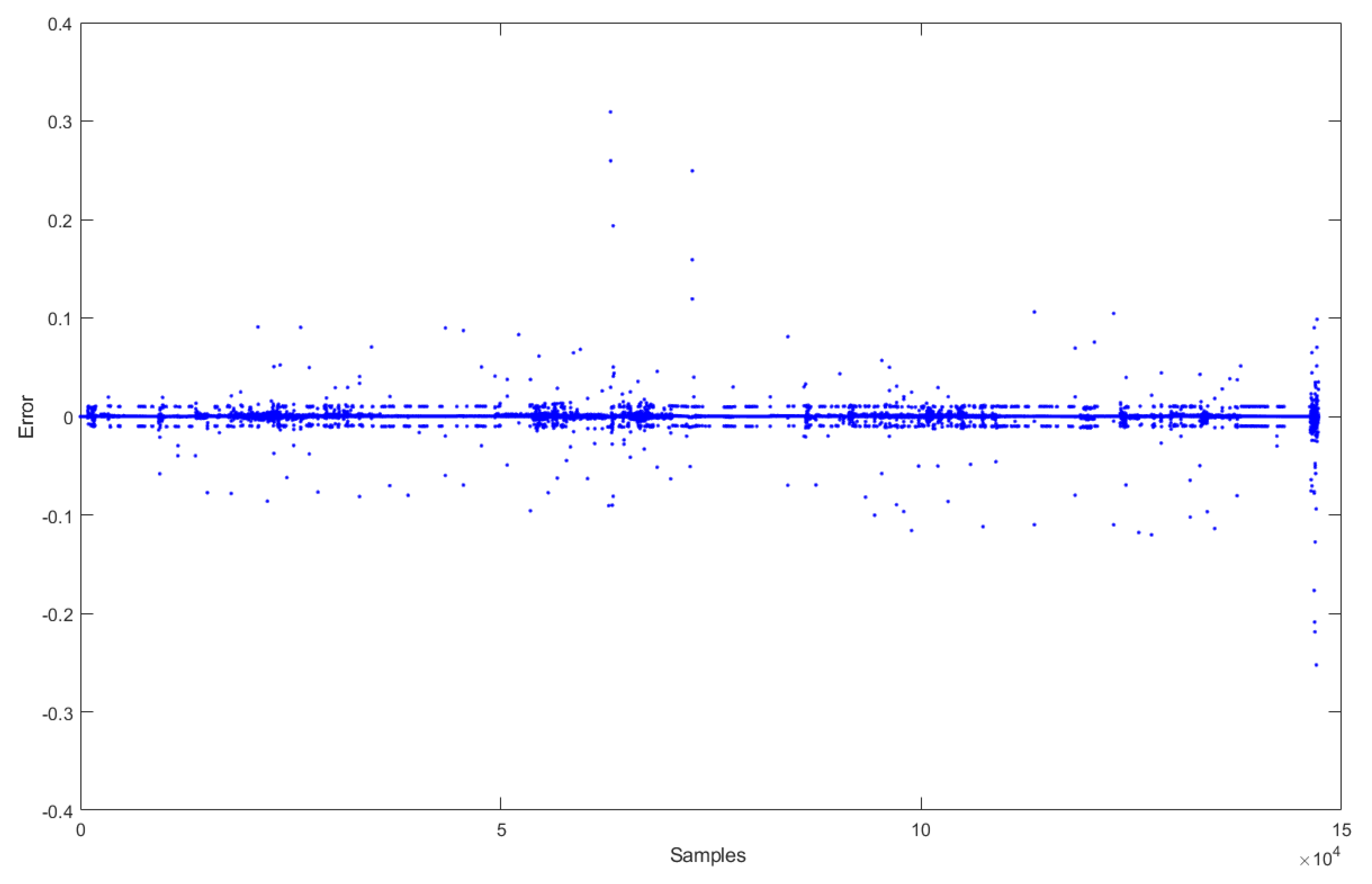
4.4. Test Results
5. Conclusions and Future Works
Author Contributions
Funding
Conflicts of Interest
References
- Vivas, F.; De las Heras, A.; Segura, F.; Andújar, J. A review of energy management strategies for renewable hybrid energy systems with hydrogen backup. Renew. Sustain. Energy Rev. 2018, 82, 126–155. [Google Scholar] [CrossRef]
- Ghanaatian, M.; Lotfifard, S. Control of Flywheel Energy Storage Systems in the Presence of Uncertainties. IEEE Trans. Sustain. Energy 2019, 10, 36–45. [Google Scholar] [CrossRef]
- Slocum, A.H.; Fennell, G.E.; Dundar, G.; Hodder, B.G.; Meredith, J.D.C.; Sager, M.A. Ocean Renewable Energy Storage (ORES) System: Analysis of an Undersea Energy Storage Concept. Proc. IEEE 2013, 101, 906–924. [Google Scholar] [CrossRef]
- Bruninx, K.; Dvorkin, Y.; Delarue, E.; Pandžić, H.; D’haeseleer, W.; Kirschen, D.S. Coupling Pumped Hydro Energy Storage With Unit Commitment. IEEE Trans. Sustain. Energy 2016, 7, 786–796. [Google Scholar] [CrossRef]
- Andújar, J.M.; Segura, F. Fuel cells: History and updating. A walk along two centuries. Renew. Sustain. Energy Rev. 2009, 13, 2309–2322. [Google Scholar] [CrossRef]
- De las Heras, A.; Vivas, F.; Segura, F.; Andújar, J. From the cell to the stack. A chronological walk through the techniques to manufacture the PEFCs core. Renew. Sustain. Energy Rev. 2018, 96, 29–45. [Google Scholar] [CrossRef]
- Moreira, M.V.; da Silva, G.E. A practical model for evaluating the performance of proton exchange membrane fuel cells. Renew. Energy 2009, 34, 1734–1741. [Google Scholar] [CrossRef]
- Kirubakaran, A.; Jain, S.; Nema, R. A review on fuel cell technologies and power electronic interface. Renew. Sustain. Energy Rev. 2009, 13, 2430–2440. [Google Scholar] [CrossRef]
- Paska, J.; Biczel, P.; Kłos, M. Hybrid power systems—An effective way of utilising primary energy sources. Renew. Energy 2009, 34, 2414–2421. [Google Scholar] [CrossRef]
- Bertoluzzo, M.; Buja, G. Development of Electric Propulsion Systems for Light Electric Vehicles. Ind. Inf. IEEE Trans. 2011, 7, 428–435. [Google Scholar] [CrossRef]
- De las Heras, A.; Vivas, F.; Segura, F.; Redondo, M.; Andújar, J. Air-cooled fuel cells: Keys to design and build the oxidant/cooling system. Renew. Energy 2018, 125, 1–20. [Google Scholar] [CrossRef]
- Ross, D. Power struggle [power supplies for portable equipment]. IEE Rev. 2003, 49, 34–38. [Google Scholar] [CrossRef]
- Andújar, J.M.; Segura, F.; Durán, E.; Rentería, L.A. Optimal interface based on power electronics in distributed generation systems for fuel cells. Renew. Energy 2011, 36, 2759–2770. [Google Scholar] [CrossRef]
- Segura, F.; Andújar, J.M.; Durán, E. Analog Current Control Techniques for Power Control in PEM Fuel-Cell Hybrid Systems: A Critical Review and a Practical Application. IEEE J. IE 2011, 58, 1171–1184. [Google Scholar] [CrossRef]
- Lekube, J.; Garrido, A.J.; Garrido, I.; Otaola, E. Output Power Improvement in Oscillating Water Column-based Wave Power Plants. Rev. Iberoam. Autom. Inf. Ind. 2018, 15, 145–155. [Google Scholar] [CrossRef]
- Jove, E.; Casteleiro-Roca, J.L.; Quintiá, H.; Méndez-Pérez, J.A.; Calvo-Rolle, J.L. Anomaly detection based on intelligent techniques over a bicomponent production plant used on wind generator blades manufacturing. Rev. Iberoam. Autom. Inf. Ind. 2019. [Google Scholar] [CrossRef]
- Amphlett, J.C.; Baumert, R.M.; Mann, R.F.; Peppley, B.A.; Roberge, P.R.; Harris, T.J. Performance modeling of the Ballard Mark IV solid polymer electrolyte fuel cell I. Mechanistic model development. J. Electrochem. Soc. 1995, 142, 1–8. [Google Scholar] [CrossRef]
- Amphlett, J.C.; Mann, R.F.; Peppley, B.A.; Roberge, P.R.; Rodrigues, A. A model predicting transient responses of proton exchange membrane fuel cells. J. Power Sources 1996, 61, 183–188. [Google Scholar] [CrossRef]
- Famouri, P.; Gemmen, R. Electrochemical circuit model of a PEM fuel cell. In Proceedings of the Power Engineering Society General Meeting, Toronto, ON, Canada, 13–17 July 2003; Volume 3, pp. 1436–1440. [Google Scholar] [CrossRef]
- Kim, J.; Lee, S.M.; Srinivasan, S.; Chamberlin, C.E. Modeling of proton exchange membrane fuel cell performance with an empirical equation. J. Electrochem. Soc. 1995, 142, 2670–2674. [Google Scholar] [CrossRef]
- Van Bussel, H.; Koene, F.; Mallant, R.K. Dynamic model of solid polymer fuel cell water management. J. Power Sources 1998, 71, 218–222. [Google Scholar] [CrossRef]
- Barragán, A.J.; Al-Hadithi, B.M.; Jiménez, A.; Andújar, J.M. A general methodology for online TS fuzzy modeling by the extended Kalman filter. Appl. Soft Comput. 2014, 18, 277–289. [Google Scholar] [CrossRef]
- Ziogou, C.; Voutetakis, S.; Papadopoulou, S.; Georgiadis, M. Modeling, simulation and experimental validation of a PEM fuel cell system. Comput. Chem. Eng. 2011, 35, 1886–1900. [Google Scholar] [CrossRef]
- López-Baldán, M.J.; García-Cerezo, A.; Cejudo, J.M.; Romero, A. Fuzzy modeling of a thermal solar plant. Int. J. Intell. Syst. 2002, 17, 369–379. [Google Scholar] [CrossRef]
- Ogaji, S.; Singh, R.; Pilidis, P.; Diacakis, M. Modelling fuel cell performance using artificial intelligence. J. Power Sources 2006, 154, 192–197. [Google Scholar] [CrossRef]
- Wojciechowski, S. A comparison of classification strategies in rule-based classifiers. Log. J. IGPL 2018, 26, 29–46. [Google Scholar] [CrossRef]
- Segovia, F.; Górriz, J.M.; Ramírez, J.; Martinez-Murcia, F.J.; García-Pérez, M. Using deep neural networks along with dimensionality reduction techniques to assist the diagnosis of neurodegenerative disorders. Log. J. IGPL 2018, 26, 618–628. [Google Scholar] [CrossRef] [PubMed]
- Andújar, J.M.; Bravo, J.; Peregrín, A. Stability analysis and synthesis of multivariable fuzzy systems using interval arithmetic. Fuzzy Sets Syst. 2004, 148, 337–353. [Google Scholar] [CrossRef]
- Barragán, A.J.; Al-Hadithi, B.M.; Andújar, J.M.; Jiménez, A. Formal methodology for analyzing the dynamic behavior of nonlinear systems using fuzzy logic. Rev. Iberoam. Autom. Inf. Ind. 2015, 12, 434–445. [Google Scholar] [CrossRef]
- Gordillo, F.; Aracil, J.; Alamo, T. Determining limit cycles in fuzzy control systems. IEEE Int. Conf. Fuzzy Syst. 1997, 1, 193–198. [Google Scholar] [CrossRef]
- González, G.; Angelo, C.D.; Forchetti, D.; Aligia, D. Detection and Isolation of Faults on the Rotor Side Converter of Doubly Fed Induction Generators. Rev. Iberoam. Autom. Inf. Ind. 2018, 15, 297–308. [Google Scholar] [CrossRef]
- Fontanet, J.G.G.; Cervantes, A.L.; Ortiz, I.B. Alternatives of Control for a Furuta’s Pendulum. Rev. Iberoam. Autom. Inf. Ind. 2016, 13, 410–420. [Google Scholar] [CrossRef]
- Irigoyen, E.; Miñano, G. A NARX neural network model for enhancing cardiovascular rehabilitation therapies. Neurocomputing 2013, 109, 9–15. [Google Scholar] [CrossRef]
- Márquez, J.M.A.; Piña, A.J.B.; Arias, M.E.G. A general and formal methodology for designing stable nonlinear fuzzy control systems. IEEE J. FUZZ 2009, 17, 1081–1091. [Google Scholar] [CrossRef]
- Javier Barragán, A.; Enrique, J.M.; Calderón, A.J.; Andújar, J.M. Discovering the dynamic behavior of unknown systems using fuzzy logic. Fuzzy Optim. Decis. Mak. 2018, 17, 421–445. [Google Scholar] [CrossRef]
- Subia, V.H.; Cedillo, B.L.; Ferragud, F.B.; Durá, J.H. Multi-objective Optimization in Modeling and Control for Rotary Inverted Pendulum. Rev. Iberoam. Autom. Inf. Ind. 2018, 15, 363–373. [Google Scholar] [CrossRef]
- Calvo-Rolle, J.L.; Quintian-Pardo, H.; Corchado, E.; del Carmen Meizoso-López, M.; García, R.F. Simplified method based on an intelligent model to obtain the extinction angle of the current for a single-phase half wave controlled rectifier with resistive and inductive load. J. Appl. Log. 2015, 13, 37–47. [Google Scholar] [CrossRef]
- Calvo-Rolle, J.L.; Fontenla-Romero, O.; Pérez-Sánchez, B.; Guijarro-Berdinas, B. Adaptive Inverse Control Using an Online Learning Algorithm for Neural Networks. Informatica 2014, 25, 401–414. [Google Scholar] [CrossRef]
- Jove, E.; Gonzalez-Cava, J.M.; Casteleiro-Roca, J.L.; Méndez-Pérez, J.A.; Antonio Reboso-Morales, J.; Javier Pérez-Castelo, F.; Javier de Cos Juez, F.; Luis Calvo-Rolle, J. Modelling the hypnotic patient response in general anaesthesia using intelligent models. Log. J. IGPL 2018, 27, 189–201. [Google Scholar] [CrossRef]
- Jove, E.; Antonio Lopez-Vazquez, J.; Isabel Fernandez-Ibanez, M.; Casteleiro-Roca, J.L.; Luis Calvo-Rolle, J. Hybrid Intelligent System to Predict the Individual Academic Performance of Engineering Students. Int. J. Eng. Educ. 2018, 34, 895–904. [Google Scholar]
- Jove, E.; Blanco-Rodríguez, P.; Casteleiro-Roca, J.L.; Moreno-Arboleda, J.; López-Vázquez, J.A.; de Cos Juez, F.J.; Calvo-Rolle, J.L. Attempts prediction by missing data imputation in engineering degree. In Proceedings of the International Joint Conference SOCO’17-CISIS’17-ICEUTE’17, León, Spain, 6–8 September 2017; pp. 167–176. [Google Scholar]
- Andújar, J.M.; Bravo, J.M. Multivariable fuzzy control applied to the physical-chemical treatment facility of a Cellulose factory. Fuzzy Sets Syst. 2005, 150, 475–492. [Google Scholar] [CrossRef]
- Zapata, F.E.; Galilea, J.L.; Bueno, J.O. ALCOR Project: Contributions to Optimizing Remote Robot Guidance in Intelligent Spaces. Rev. Iberoam. Autom. Inf. Ind. 2018, 15, 416–426. [Google Scholar] [CrossRef]
- Chalki, A.; Koutras, C.D.; Zikos, Y. A quick guided tour to the modal logic S4.2. Log. J. IGPL 2018, 26, 429–451. [Google Scholar] [CrossRef]
- Rincon, J.A.; Julian, V.; Carrascosa, C.; Costa, A.; Novais, P. Detecting emotions through non-invasive wearables. Log. J. IGPL 2018, 26, 605–617. [Google Scholar] [CrossRef]
- Tomás-Rodríguez, M.; Santos, M. Modelling and control of floating offshore wind turbines. Rev. Iberoam. Autom. Inf. Ind. 2019, 16, 381–390. [Google Scholar] [CrossRef]
- García, R.F.; Rolle, J.L.C.; Gomez, M.R.; Catoira, A.D. Expert condition monitoring on hydrostatic self-levitating bearings. Expert Syst. Appl. 2013, 40, 2975–2984. [Google Scholar] [CrossRef]
- Molina-Cabello, M.A.; López-Rubio, E.; M Luque-Baena, R.; Domínguez, E.; Palomo, E.J. Foreground object detection for video surveillance by fuzzy logic based estimation of pixel illumination states. Log. J. IGPL 2018, 26, 593–604. [Google Scholar] [CrossRef]
- García, R.F.; Rolle, J.L.C.; Castelo, J.P.; Gomez, M.R. On the monitoring task of solar thermal fluid transfer systems using NN based models and rule based techniques. Eng. Appl. Artif. Intell. 2014, 27, 129–136. [Google Scholar] [CrossRef]
- Quintián, H.; Calvo-Rolle, J.L.; Corchado, E. A Hybrid Regression System Based on Local Models for Solar Energy Prediction. Informatica 2014, 25, 265–282. [Google Scholar] [CrossRef]
- Quintian Pardo, H.; Calvo Rolle, J.L.; Fontenla Romero, O. Application of a low cost commercial robot in tasks of tracking of objects. Dyna 2012, 79, 24–33. [Google Scholar]
- Moreno-Fernandez-de Leceta, A.; Lopez-Guede, J.M.; Ezquerro Insagurbe, L.; Ruiz de Arbulo, N.; Graña, M. A novel methodology for clinical semantic annotations assessment. Log. J. IGPL 2018, 26, 569–580. [Google Scholar] [CrossRef]
- Alaiz Moretón, H.; Calvo Rolle, J.; García, I.; Alonso Alvarez, A. Formalization and practical implementation of a conceptual model for PID controller tuning. Asian J. Control 2011, 13, 773–784. [Google Scholar] [CrossRef]
- Rolle, J.; Gonzalez, I.; Garcia, H. Neuro-robust controller for nonlinear systems. Dyna 2011, 86, 308–317. [Google Scholar] [CrossRef]
- Gonzalez-Cava, J.M.; Reboso, J.A.; Casteleiro-Roca, J.L.; Calvo-Rolle, J.L.; Méndez Pérez, J.A. A novel fuzzy algorithm to introduce new variables in the drug supply decision-making process in medicine. Complexity 2018, 2018. [Google Scholar] [CrossRef]
- Burduk, A.; Bozejko, W.; Pempera, J.; Musial, K. On the simulated annealing adaptation for tasks transportation optimization. Log. J. IGPL 2018, 26, 581–592. [Google Scholar] [CrossRef]
- Casteleiro-Roca, J.L.; Barragán, A.J.; Segura, F.; Calvo-Rolle, J.L.; Andújar, J.M. Intelligent hybrid system for the prediction of the voltage-current characteristic curve of a hydrogen-based fuel cell. Rev. Iberoam. Autom. Inf. Ind. 2019, 16, 492–501. [Google Scholar] [CrossRef]
- de la Portilla, M.P.; Piñeiro, A.L.; Sánchez, J.A.S.; Herrera, R.M. Dynamic Modelling and Control of a Submerged Device with Hydrostatic Actuators. Rev. Iberoam. Autom. Inf. Ind. 2017, 15, 12–23. [Google Scholar] [CrossRef]
- Andújar, J.M.; Segura, F.; Vasallo, M.J. A suitable model plant for control of the set fuel cell–DC/DC converter. Renew. Energy 2008, 33, 813–826. [Google Scholar] [CrossRef]
- Ballard. FCgen1020-ACS fuel cell from Ballard Power Systems. Available online: http://www.ballard.com/docs/default-source/backup-power-documents/fcgen-1020acs.pdf (accessed on 15 October 2018).
- Mehta, V.; Cooper, J. Review and analysis of PEM fuel cell design and manufacturing. J. Power Sources 2003, 114, 32–53. [Google Scholar] [CrossRef]
- Ralph, T.; Hards, G.; Keating, J.; Campbell, S.; Wilkinson, D.; Davis, M.; St-Pierre, J.; Johnson, M. Low cost electrodes for proton exchange membrane fuel cells: Performance in single cells and Ballard stacks. J. Electrochem. Soc. 1997, 144, 3845–3857. [Google Scholar] [CrossRef]
- Ballard. FCgenTM-1020ACS/FCvelocityTM-1020ACS Fuel Cell Stack. Ballard Product Manual and Integration Guide. Document Number MAN5100192-0GS. Available online: https://www.ballard.com/fuel-cell-solutions/fuel-cell-power-products/fuel-cell-stacks (accessed on 9 November 2019).
- Segura, F.; Andújar, J. Step by step development of a real fuel cell system. Design, implementation, control and monitoring. Int. J. Hydrog. Energy 2015, 40, 5496–5508. [Google Scholar] [CrossRef]
- Segura, F.; Andújar, J. Modular PEM fuel cell SCADA & simulator system. Resources 2015, 4, 692–712. [Google Scholar] [CrossRef]
- Segura, F.; Bartolucci, V.; Andújar, J. Hardware/software data acquisition system for real time cell temperature monitoring in air-cooled polymer electrolyte fuel cells. Sensors (Switzerland) 2017, 17, 1600. [Google Scholar] [CrossRef] [PubMed]
- Li, X.; Deng, Z.H.; Wei, D.; Xu, C.S.; Cao, G.Y. Parameter optimization of thermal-model-oriented control law for PEM fuel cell stack via novel genetic algorithm. Energy Convers. Manag. 2011, 52, 3290–3300. [Google Scholar] [CrossRef]
- MacQueen, J. Some methods for classification and analysis of multivariate observations. In Proceedings of the Fifth Berkeley Symposium on Mathematical Statistics and Probability, Oakland, CA, USA, 21 June–18 July 1965 and 27 December 1965–7 January 1966; Volume 1, pp. 281–297. [Google Scholar]
- Moody, J.; Darken, C. Fast Learning in Networks of Locally-Tuned Processing Units. Neural Comput. 1989, 1, 281–294. [Google Scholar] [CrossRef]
- Viñuela, P.; León, I. Redes de Neuronas Artificiales: Un Enfoque Práctico; Pearson Educación: Prentice Hall, NJ, USA, 2004. [Google Scholar]
- Orallo, J.; Quintana, M.; Ramírez, C. Introducción a la Minería de Datos; Editorial Alhambra S.A.: Madrid, Spain, 2004. [Google Scholar]
- Galipienso, M.; Quevedo, M.; Pardo, O.; Ruiz, F.; Ortega, M. Inteligencia Artificial. Modelos, Técnicas y áreas de Aplicación; Editorial Paraninfo: Madrid, Spain, 2003. [Google Scholar]
- González, J.; Hernando, V. Redes Neuronales Artificiales: Fundamentos, Modelos y Aplicaciones; Ra-Ma: Madrid, Spain, 2000. [Google Scholar]
- Harston, A.M.C.; Pap, R. Handbook of Neural Computing Applications; Elsevier Science: Amsterdam, The Netherlands, 2014. [Google Scholar]
- del Brío, B.; Molina, A. Redes Neuronales y Sistemas Borrosos; Ra-Ma: Madrid, Spain, 2006. [Google Scholar]
- López, R.; Fernández, J. Las Redes Neuronales Artificiales; Netbiblo S.L.: Oleiros, Spain, 2008. [Google Scholar]
- Bishop, C. Pattern Recognition and Machine Learning (Information Science and Statistics); Springer-Verlag New York, Inc.: Secaucus, NJ, USA, 2006. [Google Scholar]
- Casteleiro-Roca, J.L.; Barragán, A.J.; Segura, F.; Calvo-Rolle, J.L.; Andújar, J.M. Fuel cell output current prediction with a hybrid intelligent system. Complexity 2019, 2019. [Google Scholar] [CrossRef]
- Heiberger, R.; Neuwirth, E. Polynomial regression. In R Through Excel; Springer: New York, NY, USA, 2009; pp. 269–284. [Google Scholar] [CrossRef]
- Wu, X. Optimal Designs for Segmented Polynomial Regression Models and Web-Based Implementation of Optimal Design Software; State University of New York at Stony Brook: Stony Brook, NY, USA, 2007. [Google Scholar]
- Zhang, Z.; Chan, S. On kernel selection of multivariate local polynomial modelling and its application to image smoothing and reconstruction. J. Signal Process. Syst. 2011, 64, 361–374. [Google Scholar] [CrossRef]


| Cl-1 | Cl-2 | Cl-3 | Cl-4 | Cl-5 | Cl-6 | Cl-7 | Cl-8 | Cl-9 | Cl-10 | |
|---|---|---|---|---|---|---|---|---|---|---|
| Global | 441,785 | |||||||||
| Hybrid 2 | 201,384 | 240,401 | ||||||||
| Hybrid 3 | 118,308 | 154,026 | 169,451 | |||||||
| Hybrid 4 | 83,452 | 86,605 | 117,997 | 153,731 | ||||||
| Hybrid 5 | 34,942 | 83,221 | 83,286 | 86,605 | 153,731 | |||||
| Hybrid 6 | 34,942 | 66,739 | 83,221 | 83,286 | 86,310 | 87,287 | ||||
| Hybrid 7 | 7785 | 27,157 | 66,739 | 83,221 | 83,286 | 86,310 | 87,287 | |||
| Hybrid 8 | 7785 | 27,157 | 37,172 | 51,646 | 65,208 | 83,221 | 83,286 | 86,310 | ||
| Hybrid 9 | 7785 | 27,157 | 30,610 | 36,146 | 37,089 | 50,181 | 83,221 | 83,286 | 86,310 | |
| Hybrid 10 | 7785 | 19,961 | 27,157 | 30,610 | 36,146 | 37,089 | 50,181 | 66,478 | 83,093 | 83,285 |
| Cl-1 | Cl-2 | Cl-3 | Cl-4 | Cl-5 | Cl-6 | Cl-7 | Cl-8 | Cl-9 | Cl-10 | |
|---|---|---|---|---|---|---|---|---|---|---|
| Global | 0.0123 | |||||||||
| Hybrid 2 | 0.0108 | 0.0149 | ||||||||
| Hybrid 3 | 0.0111 | 0.0130 | 0.0091 | |||||||
| Hybrid 4 | 0.0089 | 0.0073 | 0.0114 | 0.0122 | ||||||
| Hybrid 5 | 0.0269 | 0.0120 | 0.0054 | 0.0068 | 0.0124 | |||||
| Hybrid 6 | 0.0269 | 0.0149 | 0.0121 | 0.0053 | 0.0072 | 0.0095 | ||||
| Hybrid 7 | 0.1104 | 0.0026 | 0.0138 | 0.0123 | 0.0053 | 0.0069 | 0.0095 | |||
| Hybrid 8 | 0.1104 | 0.0027 | 0.0069 | 0.0092 | 0.0140 | 0.0121 | 0.0053 | 0,0071 | ||
| Hybrid 9 | 0.1104 | 0.0029 | 0.0199 | 0.0049 | 0.0069 | 0.0092 | 0.0108 | 0.0054 | 0.0069 | |
| Hybrid 10 | 0.1104 | 0.0069 | 0.0027 | 0.0162 | 0.0040 | 0.0068 | 0.0094 | 0.0068 | 0.0122 | 0.0054 |
| Cl-1 | Cl-2 | Cl-3 | Cl-4 | Cl-5 | Cl-6 | Cl-7 | Cl-8 | Cl-9 | Cl-10 | |
|---|---|---|---|---|---|---|---|---|---|---|
| Global | ANN12 | |||||||||
| Hybrid 2 | ANN14 | Poly1 | ||||||||
| Hybrid 3 | ANN14 | ANN12 | ANN13 | |||||||
| Hybrid 4 | ANN11 | ANN11 | Poly1 | ANN11 | ||||||
| Hybrid 5 | Poly1 | Poly2 | Poly1 | ANN12 | ANN11 | |||||
| Hybrid 6 | Poly2 | ANN13 | Poly2 | Poly1 | ANN14 | ANN13 | ||||
| Hybrid 7 | Poly1 | ANN11 | ANN13 | Poly1 | Poly1 | ANN15 | ANN11 | |||
| Hybrid 8 | Poly1 | ANN15 | ANN13 | ANN14 | ANN11 | Poly2 | Poly1 | ANN14 | ||
| Hybrid 9 | Poly1 | ANN13 | ANN11 | ANN15 | ANN15 | ANN15 | ANN13 | Poly1 | ANN15 | |
| Hybrid 10 | Poly1 | ANN15 | ANN14 | ANN11 | ANN15 | ANN13 | ANN12 | ANN14 | Poly1 | Poly1 |
| Global | Hybrid Model (Local Models) | ||||||||
|---|---|---|---|---|---|---|---|---|---|
| 2 | 3 | 4 | 5 | 6 | 7 | 8 | 9 | 10 | |
| 0.1403 | 0.1405 | 0.1466 | 0.2567 | 0.6253 | 0.9691 | 0.3424 | 0.1204 | 0.2638 | 0.2015 |
| MSE | NMSE | MAE | MAPE | |
|---|---|---|---|---|
| 8 local models configuration |
© 2019 by the authors. Licensee MDPI, Basel, Switzerland. This article is an open access article distributed under the terms and conditions of the Creative Commons Attribution (CC BY) license (http://creativecommons.org/licenses/by/4.0/).
Share and Cite
Casteleiro-Roca, J.-L.; Barragán, A.J.; Manzano, F.S.; Calvo-Rolle, J.L.; Andújar, J.M. Fuel Cell Hybrid Model for Predicting Hydrogen Inflow through Energy Demand. Electronics 2019, 8, 1325. https://doi.org/10.3390/electronics8111325
Casteleiro-Roca J-L, Barragán AJ, Manzano FS, Calvo-Rolle JL, Andújar JM. Fuel Cell Hybrid Model for Predicting Hydrogen Inflow through Energy Demand. Electronics. 2019; 8(11):1325. https://doi.org/10.3390/electronics8111325
Chicago/Turabian StyleCasteleiro-Roca, José-Luis, Antonio Javier Barragán, Francisca Segura Manzano, José Luis Calvo-Rolle, and José Manuel Andújar. 2019. "Fuel Cell Hybrid Model for Predicting Hydrogen Inflow through Energy Demand" Electronics 8, no. 11: 1325. https://doi.org/10.3390/electronics8111325
APA StyleCasteleiro-Roca, J.-L., Barragán, A. J., Manzano, F. S., Calvo-Rolle, J. L., & Andújar, J. M. (2019). Fuel Cell Hybrid Model for Predicting Hydrogen Inflow through Energy Demand. Electronics, 8(11), 1325. https://doi.org/10.3390/electronics8111325