Abstract
The growth of the world’s energy demand over recent decades in relation to energy intensity and demography is clear. At the same time, the use of renewable energy sources is pursued to address decarbonization targets, but the stochasticity of renewable energy systems produces an increasing need for management systems to supply such energy volume while guaranteeing, at the same time, the security and reliability of the microgrids. Locally distributed energy storage systems (ESS) may provide the capacity to temporarily decouple production and demand. In this sense, the most implemented ESS in local energy districts are small–medium-scale electrochemical batteries. However, hydrogen systems are viable for storing larger energy quantities thanks to its intrinsic high mass-energy density. To match generation, demand and storage, energy management systems (EMSs) become crucial. This paper compares two strategies for an energy management system based on hydrogen-priority vs. battery-priority for the operation of a hybrid renewable microgrid. The overall performance of the two mentioned strategies is compared in the long-term operation via a set of evaluation parameters defined by the unmet load, storage efficiency, operating hours and cumulative energy. The results show that the hydrogen-priority strategy allows the microgrid to be led towards island operation because it saves a higher amount of energy, while the battery-priority strategy reduces the energy efficiency in the storage round trip. The main contribution of this work lies in the demonstration that conventional EMS for microgrids’ operation based on battery-priority strategy should turn into hydrogen-priority to keep the reliability and independence of the microgrid in the long-term operation.
1. Introduction
The world energy demand is peaking over the past decades as a result of energy intensity and demographic growth [1]. At the same time, with the challenging targets of Renewable Energy Sources (RES), energy conversion systems deployment are globally pursued to address the decarbonization of the energy sector [2,3]. The increase of the penetration of stochastic renewable energy systems (such as wind and solar photovoltaic (PV) systems) produces an increasing need for control and management systems to supply such energy volume while guaranteeing, at the same time, the security and reliability of microgrids.
Locally distributed energy storage systems (ESS) [4,5,6,7] may provide the capacity to temporally decouple production and demand, providing versatility and flexibility in the operation of the microgrid. In particular, the most implemented ESS in local districts are small–medium-scale electrochemical batteries [8]. However, hydrogen systems are also viable as ESS for storing larger energy quantities over the long term thanks to the intrinsic high mass-energy density of hydrogen (Lower Heating Value LHV equal to 33 kWh/kg) which can be implemented in modular systems [9,10,11,12,13,14,15]. In this sense, hydrogen can play a key role as storage media over the long term. The correct balance between power and energy should be pursued following the specific operational requirements.
To match generation, load and storage, energy management strategies become of crucial importance: the development and implementation of control strategies that manage the power fluxes are fundamental to maintain and optimize the reliability, efficiency and operation of the microgrid in a distributed topology [16]. For the case of small-to-medium scale capacities (from several kW up to hundreds of kW or even few MW) intensive research has been made to study the behavior of hybrid renewable microgrids both connected to the main power grid or in island mode [17,18,19,20].
The control mechanisms described in the literature range from simple power balance strategies based on control variable monitoring (maintaining each component in its suitable operation condition range) [5,6,21,22], up to complex control strategies such as load management based on baseload and peak load [23] hierarchical control (master-slave) [24,25], model predictive control [4,26], global optimization via objective functions [27], self-optimization strategies [24] and fuzzy logic [27,28,29] and genetic algorithms [30]. Hydrogen-priority strategy in small scale hybrid microgrids with a hydrogen battery storage system is quite uncommon in scientific literature, except for few studies with combined solutions [6,21,31] or hydrogen-only storage systems [4]. Battery-priority strategies are the typical high-level control systems implemented for short/medium-term microgrid management found in the literature [5,20,22,27,30,32]. A comprehensive review of different microgrid management systems can be found in [33].
In this paper, an energy management system (EMS) with two strategies based on hydrogen-priority and battery-priority is proposed for the operation of a hybrid renewable microgrid, implementing selective power balance based on the control variable monitoring. The aim of the comparison is to assess the microgrid’s performance in the long-term regarding the internal reliability of the microgrid and energy efficiency. Hydrogen can exploit the greater energy inertia to lead the microgrid towards island operation (zero support from the main power grid). On the other hand, the battery-priority approach attempts to minimize the amount of energy lost in the storage round trip, since the nominal efficiency of battery systems is considerably higher than the one of hydrogen systems. Respect to most of the analyzed literature, which attempts to optimize the real-time operation of the microgrid from an electrical point of view with simulations in the short-term [20], the main novelty of this paper is it investigates the microgrid performance in the long-term from an electrical and energetic standpoint. The evaluation is done over an annual timescale under both strategies: hydrogen-priority compared to a typical battery-priority. The results obtained endorse the main contribution of the paper: an analysis about EMS based on battery-priority, as widely extended, regarding hydrogen-priority in the long-term microgrid operation. The paper demonstrates that the hydrogen-priority EMS strategy guarantees better reliability and independence in long-term operation.
2. Materials and Methods
The conception of the microgrid is based on the production of energy entirely obtained from renewable resources, which guarantees the production and storage of energy with zero CO2 emissions. The microgrid includes different RES power generation systems on several kW scales, together with similar scale hydrogen and battery storage systems. The architecture integrates a mixed type, AC/DC electrical topology presenting a high-voltage DC bus (400 V DC) and a standard 1ph-230 V/3ph-400V AC bus, Figure 1 [22].
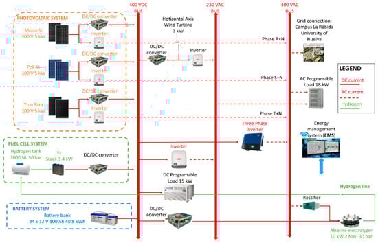
Figure 1.
The hybrid renewable microgrid at the University of Huelva.
Considering the topology of the renewable microgrid under study, which is located in the “La Rábida” Campus, at the University of Huelva (Huelva is located in the southwest of Spain), it allows bidirectional power flow between the main power grid and the microgrid. Considering the integration method, all the generation and consumption systems are connected to the internal DC bus, supported by the direct connection of the battery bank.
The renewable generation part is provided by variable renewable resources (solar radiation and wind), which allow the production of energy upon resource availability. The microgrid facility can be operated supplying the real demand of the “La Rábida” Campus or to satisfy any desired consumption profile. This can be done, see Figure 1, through programmable power sources and loads. To guarantee the power balance at all times, there are two ESSs available. The first ESS is a battery bank; the direct connection of the battery bank to the internal DC bus causes the voltage of DC bus to be stabilized within the operating range of the battery bank, without the need of using additional bidirectional converters that could complicate the control of the system. The second ESS is a hydrogen loop, consisting of an electrolyzer (hydrogen producer), a fuel cell (hydrogen consumer) and a compressed hydrogen storage tank.
The energy conversion systems and buses are connected by means commercial and customized power electronic converters. The connected and operating systems are reported in Table 1.

Table 1.
Technical characteristics of components from microgrid shown in Figure 1.
After the microgrid its components have been described in the next section, the following section will show the modelling process developed. The objective is to obtain a customizable model to evaluate energy strategies over the microgrid operating in the long-term.
3. Modelling of the Microgrid Components
In general, the proposed component modelling approach is an intermediate step between system and process modelling; in fact, the objective is to obtain an easily customizable model to assess energy dispatch strategies over yearly simulations in an hourly timestep, without considering transients and local controllers that operate on the order of seconds. It is supposed that each component will be equipped with an internal control loop that ensures the component operates in a suitable way (Maximum Power Point Tracking MPPT algorithms for solar PV, blade pitch control and par regulation for wind turbines, charge controllers for batteries, etc.) [20,24,25,27].
The proposed model simulates one year (8760 h) with a discrete time step of one hour. An entire yearly simulation is computed in approximately one minute of simulation, which represents an acceptable balance between accuracy and computational load to analyze the microgrid response in the long term.
In the following sections, each component model is discussed in detail. An error analysis is presented in order to validate the modelling of all the components with respect to the real measured values under the same operating conditions of the real equipment operating in the real microgrid in Huelva. The error analysis is presented in terms of average relative error , Root Mean Square Error (RMSE) and Normalized Root Mean Square Error (NRMSE). Their precise definition has been included in the Notation and Symbols list. The error analysis is reported for each component in the following Section 3.1, Section 3.2, Section 3.3, Section 3.4, Section 3.5, Section 3.6.
3.1. Solar PV Model
The microgrid in Figure 1 has 15 kW p of solar PV installed (Figure 2), divided into three modules of 5 kW p of monocrystalline and polycrystalline amorphous thin film Si-based technology. The 300 V solar arrays are connected at the main switchboard in series. By default, the PV production is sent to an inverter and injected into the main power grid but can be connected directly to the 400 VDC bus by switching to the DC-DC converters which assure voltage coupling.
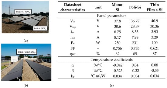
Figure 2.
(a,b) Detail of the solar PV installation of microgrid shown in Figure 1; (c) PV panels datasheet characteristics.
The model implemented is taken from [34,35]; it is based on inclined radiation and panel temperature correction of the short circuit current, , and open-circuit voltage, , Equations (1) and (2). The total electrical power output of the panel array is calculated by multiplying current and voltage, equation (3), taking into account the panel array configuration. The panel temperature is calculated from the measured ambient temperature by considering a global heat transfer coefficient kp (°C m2/W) [36] which takes into account the global conductive, convective and irradiation heat inputs to the panel. Equations (1) and (2) are taken from [34,35]:
Multiplying obtained from (1) and obtained from (2) and taking into account the array configuration and losses up to the DC terminals of the inverter, it is possible to know the total PV power at the each solar field:
where:
- is the current correction factor given in the datasheet (%/°C) (see Figure 2c)
- is the voltage correction factor given in the datasheet (%/°C) (see Figure 2c)
- is a non-dimensional correction coefficient (−0.04 [34])
- is fill factor given in the datasheet (-) (see Figure 2c)
- is the measured global inclined radiation (W/m2)
- is the global radiation at STC conditions (1000 W/m2)
- is the short-circuit current (A)
- is the short-circuit current at STC conditions (A) (see Figure 2c)
- is the number of panels in series (20)
- is the number of panels in parallel (1)
- is the total efficiency up to the DC switchboard (considering electrical, atmospheric, shadowing and soiling losses in each particular installation) (see Figure 2c)
- is the solar panel electrical power output (W)
- is the measured panel temperature (°C)
- is the temperature at STC conditions (25 °C)
- is the open-circuit voltage (V)
- is the open-circuit voltage at STC conditions (V) (see Figure 2c)
For each technology, the output power results as two independent variables function, represented in the case of monocrystalline silicon in Figure 3a. The parametrical temperature and radiation effect are shown in Figure 3b.
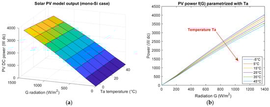
Figure 3.
(a) Solar PV modelling; (b) PV power output vs temperature and radiation (model).
To validate the proposed model with experimental data, Figure 4 shows the daily power production for the three technologies of Figure 2, by running a full-day simulation with the locally acquired meteorological data and the experimental measurements.
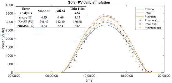
Figure 4.
Validation of the solar PV model for the three technologies and error analysis.
It can be seen that the model follows within a reasonable approximation of the experimental measurements (Figure 4). As assessed in the figure, in all cases the average error committed by the model is below 5% of the measured values and the normalized error is below 5% of the nominal power of the PV systems.
3.2. Wind Turbine Model
On the same rooftop as the solar PV systems, a 3 kW horizontal axis micro wind turbine is installed as shown in Figure 5a. The nominal parameters of the wind turbine are reported in Figure 5b. Similarly to the PV system, by default the wind turbine injects power to the microgrid but can be set in island mode by switching the connection to the electrical converters which can connect the wind turbine either to the AC or to the DC bus (Figure 1).
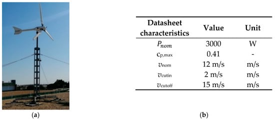
Figure 5.
(a) Horizontal axis wind turbine of the Figure 1 microgrid; (b) wind turbine datasheet parameters.
The 3-kW rated wind turbine will be modelled by implementing its power curve with a cubic curve as reported in the technical datasheet with a resolution of 1 m/s, Equation (4). The characteristic values of cut-in and cut-off speeds determine the limits of operation of the wind turbine. The nominal wind speed determines the value from which the power output goes from a cubic function to a constant, thanks to the variable pitch regulation (which is not detailed in this paper) of the turbine blades [37]. In the model of equation (4), constant electrical, mechanical and aerodynamic efficiency factors are considered, equal to 85%, 90% and 90% respectively.
where:
- is the wind turbine model fit parameter (−8.1987)
- is the wind turbine model fit parameter (180.86)
- is the wind turbine model fit parameter (−911.62)
- is the wind turbine model fit parameter (1352.2)
- is the electrical efficiency (85%)
- is the mechanical efficiency (90%)
- is the aerodynamic efficiency (90%)
- is the power developed by the wind turbine (W) in function of the wind speed (m/s)
- is the nominal power developed by the wind turbine (W) (see Figure 5b)
- is the measured wind speed (m/s)
- is the cut-in speed given in the datasheet (m/s) (see Figure 3b)
- is the cut-off wind speed given in the datasheet (m/s) (see Figure 5b)
- is the nominal wind speed given in the datasheet (m/s) (see Figure 5b).
By feeding the model with the daily wind speed values for the selected days, it is possible to validate the model (Figure 6) by comparing the results with the actual power injected to the microgrid.
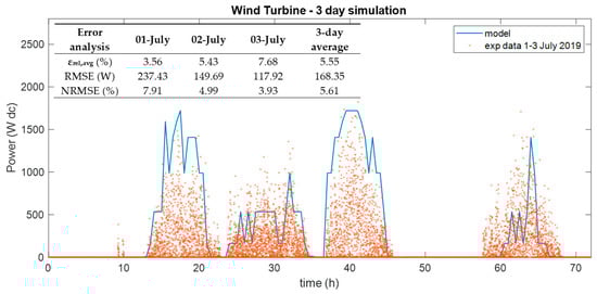
Figure 6.
Validation of the wind turbine model and error analysis.
As can be seen in Figure 6, the power output obtained by the model (in blue) follows the trend of the experimental data (in orange) with a rather good approximation. The average relative error on a daily basis is below 8% (the worst case is 03/07) and on average throughout the three days below 6%. The average RMSE normalized respect to the nominal power of the wind turbine is also below 6%. It is assumed that, in the long-term annual simulations, the error is smoothened by the increasing amount of data.
3.3. Alkaline Electrolyzer Model
The microgrid is provided with a 10 kWe alkaline electrolyzer (Figure 7a) with datasheet characteristics shown in Figure 7b; the nominal production is 2 Nm3/h of hydrogen. The produced gas is stored, at the outlet pressure of the electrolyzer (30 bar), in a tank, Figure 7a.
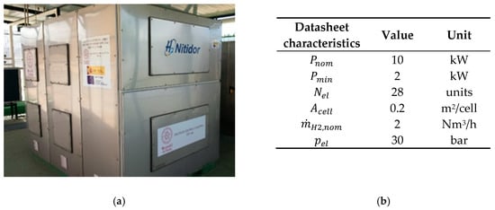
Figure 7.
Details of the alkaline electrolyzer (a), and datasheet characteristics (b).
The electrolyzer was modelled empirically, due to fact that the electrolyzer SCADA system only monitors the stack voltage and current allowing the imposition of a power setpoint (expressed as % of the rated power—see Figure 8b). For this reason, it was assessed to be a more suitable—from a system modelling point of view—more reliable but empirical, model-based interpolation of real data (see Figure 8a), rather than a more in-depth analytical process model without the means of validating the involved variables (for example instantaneous gas partial pressure, local cell current density distribution, water/gas flow rate), which are not accessible for measurement due to the lack of measurement systems in place required to validate a process model. In addition, the I-V curve trend and results are in line with the values reported in the literature [38].
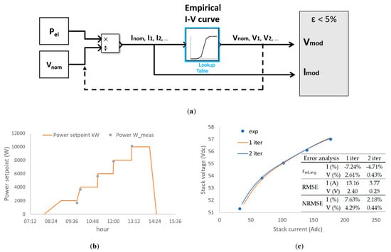
Figure 8.
(a) Alkaline electrolyzer empirical modelling scheme; (b) experimental test procedure (c) polarization curve (stack) experimental data, polynomial fitting and error analysis.
The empirical model scheme is reported in Figure 8a, interpolating the current and voltage data according to the empirical I-V curve obtained from experimental testing on the equipment. Due to the observed near-constant behavior of the voltage (from a system point of view), it is possible to derive a first iteration value of the current by simply dividing the input power setpoint by the nominal voltage. Once the first iteration current has been calculated, a second new value of voltage is calculated via a cubic spline interpolation on the empirical I-V curve. The iterative method continues, calculating a second iteration current and so on.
By applying the model to a continuous spectrum of input power from 2 kWe to 10 kWe (20%–100% of the nominal power) the correspondence of the output current and voltage simulated values respect to the measurements is verified, Figure 8b,c. The results can be refined by iterating the process until a suitable accuracy is reached (εrel <~5% for both current and voltage).
The validation of the model confirms that, from a system point of view, the electrolyzer could be in the first approximation represented by constant voltage and linear current to match the power setpoint. It has been found that, already at the second iteration, the voltage reduces its average error to 0.43%, and the current reduces its average relative error with respect to the experimental values from -7.240% to -4.708%.
To calculate the hydrogen flow it is possible to apply Faraday’s Law to obtain the molar flow from the stoichiometry of the reaction, Equation (5).
where:
- F is the Faraday constant (96485 C/mole-)
- is the measured electrolyzer current (A)
- is the electrolyzer cells number (28 units)
- is the Faraday efficiency (98.5%)
- is the molar flow of hydrogen (mol/s)
- z is the number of moles of electrons per mole of hydrogen (2 mole-/molH2).
The Faraday efficiency is instead dependent on the current density and can be calculated with the model proposed by Ulleberg [38], at the operating temperature of 60 °C, maintained constant by the cooling system.
3.4. PEM Fuel Cell Model
The PEM fuel cell that is part of the microgrid (Figure 9a) is made up of a stack with 80 single planar cells in series, with an active surface of 0.0145 m2/cell [39]. Its nominal power is 3.4 kWe, but due to stack degradation the actual power is limited by the control system to 2 kWe. Datasheet characteristics are reported in Figure 9b.
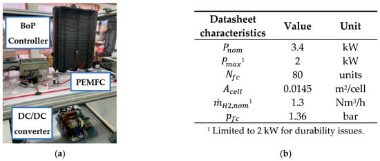
Figure 9.
Details of the PEM fuel cell module (a) and datasheet characteristics (b).
Empirical I-V curves were obtained by applying a third-order polynomial fit—Equation (6)—according to the cubic spline interpolation method with respect to experimental I-V measurements obtained by testing one fuel cell unit over a power setpoint range from 0 to 2 kW—Figure 10a. Since the fuel cell power is limited to 2 kWe [40], the fuel cell output power can be considered linear with reasonable approximation, Equation (7) and Figure 10b, since the concentration loss region is not reached. By knowing the input power setpoint of the system, the operating current in the linear region can be determined from the I-P curve; successively, by entering the I-V curve with the found value of current, the voltage can be determined. The committed average relative error is below 2% with respect to the median of the experimental values, which are affected by hysteresis in the measured power setpoint range. The trend of the obtained curves shows correspondence with the literature-reported data [41,42].
where:
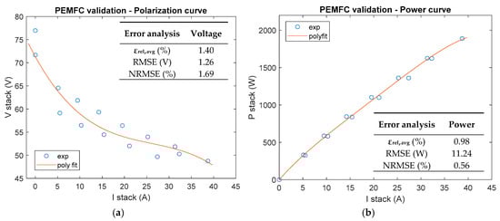
Figure 10.
(a) Fuel cell polarization curves. Experimental data vs. polynomial fitting model; (b) Fuel cell power curves. Experimental data vs. polynomial fitting model.
- is the fuel cell model fit parameter (73.326)
- is the fuel cell model fit parameter (−2.122)
- is the fuel cell fit parameter (0.077)
- is the fuel cell fit parameter (−0.001)
- is the fuel cell current (A)
- is the fuel cell voltage (V).
Similarly to the electrolyzer case, from the measured fuel cell current it is possible to obtain the molar flow from Faraday’s Law, Equation (8). Via successive measurement unit conversions, it is possible to obtain volumetric and mass flow for each operating point.
where:
- F is the Faraday constant (96485 C/mole-)
- is the fuel cell current (A)
- is the number of cells in the fuel cell (80 units)
- is the Faraday efficiency (99%)
- is the molar flow of hydrogen (mol/s)
- z is the number of moles of electrons per mole of hydrogen (2 mole-/molH2)
The Faraday efficiency is calculated in the same way described for the electrolyzer [38] but at 40 °C, maintained isothermally by the PEM cooling system.
3.5. Compressed Hydrogen Storage Tank Model
Hydrogen produced from the electrolyzer supplying to the fuel cell is stored in a tank with a volume of 1.044 m3 and a nominal pressure of 30 bar, Figure 11.
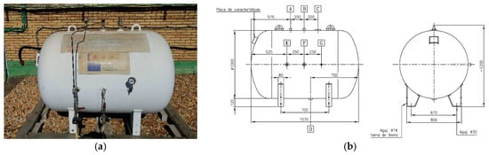
Figure 11.
(a) Detail of the hydrogen compressed gas tank; (b) layout characteristics.
Hydrogen can be considered as a perfect gas throughout the whole pressure and temperature range of operation for compressed hydrogen storage [43]. Under this hypothesis, in isothermal conditions, density is linear with pressure and a linear relationship between pressure and molar quantity can be obtained by applying the perfect gases law, Equation (9) [24]:
where:
- is the hydrogen molar variation (mol)
- is the pressure variation (atm)
- is the perfect gas constant (0.082 atm.L/mol.k)
- is the gas temperature (293 K)
- is the geometrical tank volume (1.044 L).
The effect of temperature is neglected since the storage tank is stationary and the hydrogen flow rate is limited.
3.6. Lead-acid Battery Model
A battery bank composed of 34 units of 100 Ah 12 V, based on lead-acid technology, Figure 12a, in series is directly connected to the DC bus (see Figure 1). Each battery is composed of six elementary cells in series and the 34 units are connected in series to reach the 400 Vdc of the DC bus. The datasheet characteristics of the battery bank (single 12 V; 100 Ah unit) are reported in Figure 12b.
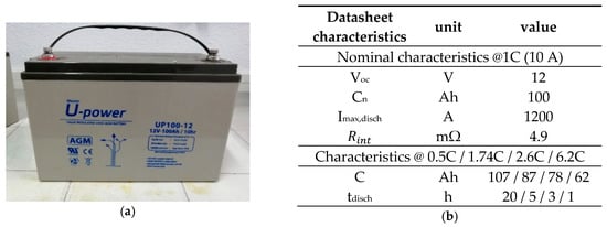
Figure 12.
(a) Lead acid battery unit; (b) lead acid battery datasheet characteristics [44].
Actual data of current, voltage and state of charge (SOC) obtained from a test-bench during multiple charge/discharge cycles protocols were utilized in order to fit an empirical two-variable ( and SOC) model for the calculation of the battery voltage, differentiating between charge and discharge phases. The chosen model was proposed by Tremblay [45] and adapted by Valverde et. al. [31,41]; it consists of two separate relations during charge (> 0) and discharge (< 0) phases, Equations (10) and (11). The SOC value has been calculated according to the Coulomb counting method [27,41] and corrected according to the real battery capacity obtained by Peukert’s Law [46], Equation (12).
where:
- is the exponential zone amplitude (V) (see Table 2)
Table 2. Battery experimental data fitting results via MATLAB Curve Fitting Toolbox.
- is the exponential zone time constant inverse (Ah−1) (see Table 2)
- is the battery nominal capacity (100 Ah)
- is the battery current (A) (negative for discharge and positive for charge)
- is the polarization resistance (Ω) (see Table 2)
- is the battery internal resistance (4.9 mΩ)
- is the battery state of charge (Ah)
- is the initial battery state of charge (100%)
- is the time interval (h)
- is the battery voltage (V)
- is the open circuit voltage (V).
The data fitting process is taken out via MATLAB Curve Fitting Toolbox, an additional plug-in for fitting curves or surfaces to data. The tool is configured in custom equation mode—Equations (10) to (12)—using the default nonlinear least square fitting method according to the Trust-Region algorithm. and are selected as the two independent variables and the values of , and are fixed from datasheet; , and are the parameters subject to data fitting via MATLAB Curve Fitting Tool: Figure 13 and Figure 14. The data-fit results are reported in Table 2.
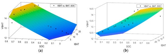
Figure 13.
(a) Battery charge experimental data fitting results via MATLAB Curve Fitting Toolbox, frontal view and (b) lateral view and error analysis.
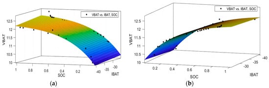
Figure 14.
(a) Battery discharge experimental data fitting results via MATLAB Curve Fitting Toolbox, frontal view and (b) lateral view and error analysis.
The discharge phase is quite linear, therefore a very good approximation (R-square = 0.971, Table 2) is obtained with the experimental data. The charge phase fitting presents more difficulty due to the non-linear charge protocol; therefore, more experimental data was required to achieve a comparable approximation (R-square = 0.959, Table 2). In fact, the higher-end SOC range is measured at constant voltage, narrowing the spectrum of available experimental data for surface fitting. In a real-case operation, it is difficult that such constant voltage charging conditions occur.
In order to validate the model, it has been applied to the experimental data of a series of five successive charge/discharge cycles. In Figure 15a, the measured voltage (in blue) is compared (below) to the voltage calculated by the model (in red) together with the relative error (Figure 15a below and Figure 15b) with respect to the measured data. Discontinuities in the voltage profile, such as the one seen in t = 5 h, are normal and due to the switch from charging to discharging mode during experimental test. It consists of multiple charging/discharging cycles applied over the battery. In the instant of the switch, the battery is put in open circuit conditions (returning to around 12 V) and then switched to the successive charge/discharge phase, allowing the voltage to vary suddenly. The model shows good accordance with the experimental data (relative error <1% and <3% normalized respect to the nominal voltage), except for the constant voltage zones during battery charge, as previously discussed.
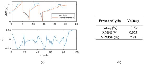
Figure 15.
(a) Lead acid battery model validation; (b) error analysis.
4. Energy Management System (EMS). Strategies Definition: Hydrogen- vs. Battery-priority
The complete microgrid model is implemented into Simulink environment in order to perform the global simulation, Figure 16. The input data are radiation, , ambient temperature, , and wind speed, obtained by PV-GIS satellite data for the microgrid geographical location (database from 2007 to 2017) [47]. A typical residential load profile has been considered [22]. Each component is parameterized according to the specifications of the simulated system, as discussed in Section 3. The sum of the solar PV power and wind turbine power consists of the total renewable power generated. The total produced power is compared in each hour timestep with the load power, resulting in a net power which should be managed by the ESSs or by the external power grid. If in a specific timestep the net power is positive (), the microgrid presents an energy excess scenario, where the produced power is greater than the demand power; on the other hand, a negative net power () means a deficit scenario where the load power is greater than the produced power. All the power in the microgrid is assumed to be exchanged via the 400 V DC bus. The net power balance is converted into power setpoints to the ESSs, which in turn translate into current setpoints which determines the charge/discharge behavior of the ESS. As a consequence, the battery SOC and the hydrogen tank pressure are calculated according to the net balance of hydrogen/battery charge quantity. The SOC and tank pressure starting values must be initialized.
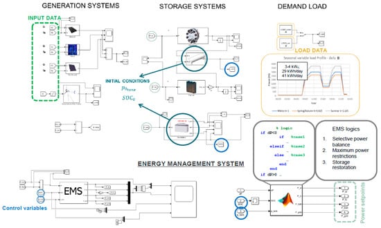
Figure 16.
Simulink global model interface.
The EMS computes the net power balance between the total RES generation and the load. According to the imposed limits of the control variables of battery State of Charge () and hydrogen stored in the tanks, computed by the tank pressure . The EMS implements a logical algorithm according to the decided priority strategy, providing the power setpoint outputs for each component (electrolyzer, fuel cell, battery and main power grid) [48]. The minimum and maximum limits of operation of each energy storage is defined according to the technology operation range [19,24], while low and high limits of each ESS are defined according to the hysteresis amplitude in relation to the restoration logic [5,22,25,30,31].
4.1. Hydrogen-priority Strategy
For the Hydrogen-priority strategy, the EMS objective is to maximize the internal reliability by increasing the hydrogen systems utilization. In fact, hydrogen allows greater inertia to be obtained due to the greater amount of energy (kWh) stored in the form of hydrogen in comparison to the batteries. This allows larger loads to be continuously supplied with more stable operation of the hydrogen storage. When the renewable energy supply is higher than the load demand (), the electrolyzer is put in work with the aim to consume the energy excess and to have energy stored in the form of hydrogen. In the other case, when solar and wind do not meet the load demand (), it will be the fuel cell the first responsible for supplying the energy deficit. After that, when the hydrogen tank pressure approaches the limit values ( and ) the system shifts the load to the batteries (both charge and discharge), provided that the SOC is in the suitable range. If the battery SOC is also not within the suitable operating range (, ), the power is supplied by or injected into the main power grid, which acts as a support or as “dump” load. To avoid continuous changes in the operation mode and to support the restoration of unavailable ESSs, a hysteresis bandwidth and logic has been defined of hydrogen systems and battery bank. That is, if useful power is available and if the complementary storage system is in a normal operating range, the hydrogen-based systems keep in near-unavailable condition.
4.2. Battery-Priority Strategy
On the other hand, in the battery-priority strategy, the battery bank is used as the primary energy backup, using the hydrogen systems only when the SOC is outside of the allowed operation range [22]. The hydrogen loop (electrolyzer and fuel cell) is used as a secondary backup when the batteries are unavailable. If both systems are outside the suitable operating range, the power is supplied by or injected into the main power grid, which acts as microgrid support or “dump” load. In a similar way, the logical structure of the strategy defines a hysteresis loop, in order to restore an unavailable ESS, prioritizing the battery bank respect to the hydrogen tank.
4.3. Strategies Comparison and Global Evaluation Parameters
The two strategies are schematized and compared in Figure 17. The system computes the net power balance between the total RES generation and the load according to the imposed limits of the control variables of battery State of Charge () and hydrogen stored in the tanks, computed by the tank pressure . The EMS implements a logical algorithm according to the decided priority strategy, providing the power setpoint outputs for each component (electrolyzer, fuel cell, battery and main power grid) [48]. The minimum and maximum limits of operation of each energy storage system are defined according to the technical operation range [19,24], while low and high limits of each ESS are defined according to the hysteresis amplitude in relation to the restoration logic [5,22,25,30,31].
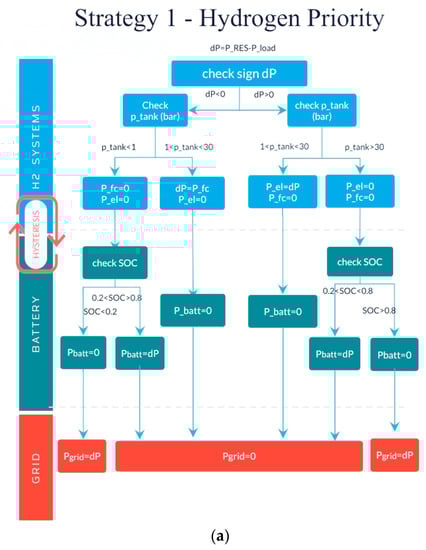
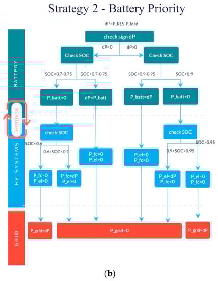
Figure 17.
Hydrogen-priority strategy (a); battery priority strategy (b).
The numerical results of the simulations must be categorized into a set of quantitative evaluation parameters (Table 3) in order to be able to compare the simulations results obtained from each strategy. These parameters are aggregate values, which embrace and represent the global system performance in the long-term.
Table 3.
Global evaluation parameters.
The cumulative annual energy is equal to the sum of the instantaneous power multiplied by the time (1 h); is the cumulative count of operating hours of each component. Where Loss of Load (LL) is the amount of energy demanded by the load but not supplied by the microgrid; Loss of Load Probability (LLP%) is the percentage of unmet load respect to the total load demand; Storage efficiency () is the ratio between the energy input to the ESSs (hydrogen production via electrolysis and battery charging) and the energy output from the ESSs (during the fuel cell operation and the battery discharging). For the Loss of Load parameter, , only the contribution from the main power grid is considered (), while the injection to the main power grid () is not considered. Load shedding or any kind of active load modification (demand response) is neglected.
5. Results
5.1. Simulation Conditions
The long-run simulations are obtained by feeding yearly data (Figure 18) with hourly resolution into the developed model. The 2016 data was used [47] which represented a worst-case scenario, since the radiation profile was on average the lowest throughout the 10 years of the database. Since the RES generation systems are predominantly solar, this represents a worst-case scenario for the storage system, which must support a more demanding energy deficit scenario.
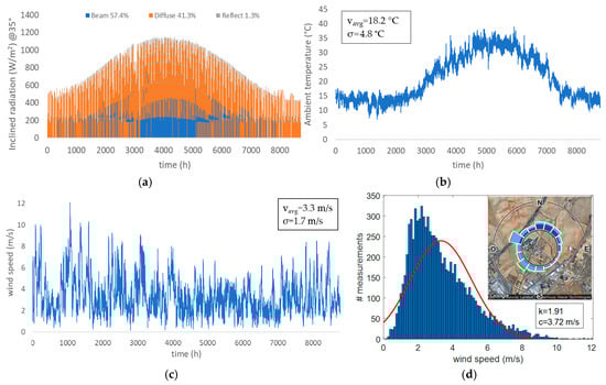
Figure 18.
Annual meteorological data on the microgrid location (Huelva, southwest of Spain). (a) Inclined solar radiation and its components; (b) ambient temperature—mean and standard deviation (σ); (c) wind speed (W10)—mean and standard deviation (σ); (d) wind statistical analysis—Weibull distribution and fitting—shape (k) and scale (c) factor.
The considered load [22] is a typical 3–4 kWp (), 35 kWh/dayavg residential type load profile as shown in Figure 19. The profile matches the typical working habits of the city environment, where the starting working hour is around 09:00–10:00, with a valley around 14:00–17:00 and the second peak from 17:00–18:00 to 21:00–22:00. The seasonal behavior of the load has been assessed by implementing a correction coefficient which takes into account the seasonal variability of cumulative energy obtained by the analysis of local loads, Figure 19a.
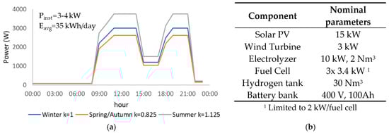
Figure 19.
(a) Load profile; (b) Simulated microgrid configuration setup.
The long-term simulation has been run for both strategies for 8760 h with a seasonal variable load, Figure 19a. Figure 19b summarizes the simulated microgrid setup, while Table 4 reports the EMS parameter configurations.
Table 4.
Hydrogen-priority and battery-priority strategies input parameters.
In this case a direct comparison of results can be made since the simulated components and conditions are the same, with only different EMS strategies.
5.2. Comparison of Simulation Results and Evaluation Indicators
The simulation results for power balance and trends of the controlled storage variables are reported in Figure 20 and Table 5 and Table 6.
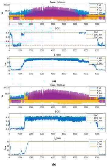
Figure 20.
Net power balance. (a) Hydrogen-priority EMS strategy results; (b) battery-priority EMS strategy results.
Table 5.
Comparison of simulation results 1. Global parameters.
Table 6.
Comparison of simulation results 2. Energy Flow.
6. Discussion
Firstly, both EMS strategies assure that the overall power balance is always met, thanks to the main power grid intervention. It can be clearly seen in Figure 20 that winter (hours 1–2190) and autumn (hours 6570–8760) seasons correspond to the main energy deficit periods of the year, due to lesser solar resources. The predominance of solar systems determines a strong energy excess scenario during spring and summer (hours 2190–6570). The overall power balance is also affected by the seasonal load (Figure 19) which is most demanding during summer and least demanding during spring/autumn.
By comparing the results, the priority relevantly affects the overall power balance; in the case of hydrogen-priority EMS strategy, the hydrogen input energy is 7286 kWh (Table 6, first row) versus only 690 kWh sent to the batteries (Table 6, third row), while in the battery-priority EMS strategy the hydrogen input energy is only 1226 kWh against 4408 kWh for the batteries. This aspect is reflected also by the amount of hydrogen used, which is equal to 1584 Nm3 for the hydrogen-priority EMS strategy (several cycles) against 165 Nm3 for the battery-priority EMS strategy (few cycles). In terms of main power grid energy, the battery-priority EMS strategy injects 9632 kWh and uses 562 kWh (Table 6, row five and six). On the other hand, the hydrogen-priority EMS strategy presents a reduced interaction with the main power grid, both in injection and support mode, respectively 7290 kWh and 254 kWh (Table 6, row five and six), which accounts for a reduction of 24% in terms of injection energy, and 55% in terms of main power grid support. Additionally, both EMS strategies were calibrated in order to accept an energy excess scenario and minimize the main power grid support. In terms of supply of the load (Table 5, first and second row), the hydrogen-priority EMS strategy achieves better performance (2.05% LLP%) against the battery-priority EMS strategy (4.54% LLP%). The difference in the LLP% is not as relevant as the difference in storage capacity due to the effect of the round-trip efficiency for the two storage pathways, greatly reducing the useful energy for the hydrogen storage. Global storage efficiency (Table 5, third row) is lower for the hydrogen-priority EMS strategy, 50.3% versus a global storage efficiency of 65.5% for the case of battery-priority EMS strategy, which is due to the differences in the main devices’ nominal efficiencies. In fact, the overall energy processed by the storage system is greater for the hydrogen-priority EMS strategy (7976 kWh versus that much less energy processed by the battery-priority EMS strategy, only 5634 kWh), which is due to the much lower energy share processed by the batteries (which present higher nominal efficiency) for a comparable output power (4055 kWh versus 3746 kWh).
The trends of the results are aligned with similar trade-off scenarios reported in the literature between energy efficiency, LLP% and system utilization, depending on the prioritization of the hydrogen or battery systems in the microgrid management [6,21].
7. Conclusions
Although the use of RES is growing in order to address decarbonization targets, the time discontinuity of renewable resources demands electrical grids topologies and EMS that can assure the demand with quality, security and reliability. In this sense, local distributed ESS offers the possibility to temporarily decouple production and demand, providing versatility and flexibility in the operation of the renewable electrical grids.
With this goal in mind, this paper has presented an EMS functioning under two different strategies: hydrogen-priority vs battery-priority. The goal is to compare the results obtained when the priority is to maximize the hydrogen systems’ utilization with the results obtained when the priority is to increase the battery bank use. In both cases, the EMS pursues the best operation of the hybrid renewable microgrid, implementing a selective power balance based on the control of the microgrid in the long-term operation. The aim of the comparison between the two strategies is to analyze the long-term behavior of the EMS in terms of the microgrid performance and efficient energy use.
Under the hydrogen-priority strategy, a higher amount of energy (kWh) is stored in the form of hydrogen, allowing a greater “energy inertia” in comparison to the batteries. On the other hand, in the battery-priority strategy, the battery bank is used as primary energy backup, which presents an increased round-trip efficiency; only when the bank battery SOC is not within the allowed range, the hydrogen loop (electrolyzer and fuel cell) is used as a secondary backup.
By comparing both EMS strategies under the same simulation conditions, it has been verified that the hydrogen-priority EMS strategy achieves lower LLP values (2% vs 6% for battery-priority EMS strategy, ratio 1:3), thanks to the higher energy capacity respect to the battery storage (90 kWh vs 40 kWh, ratio 2.25:1), which is due to the mass-energy density of the hydrogen as an energy vector, providing more storage autonomy respect to the batteries. However, the global storage efficiency decreases from 65.5% to 50.3%, due to the reduced share of battery energy, whose energy conversion ratio is higher. In fact, the hydrogen-based systems process much more energy (7976 kWh against 5634 kWh when the battery-priority strategy is used) for a comparable output power (4055 kWh versus 3746 kWh), thus generating more losses.
In the reviewed literature, most works regarding hybrid renewable microgrids modelling are based on battery-priority energy management strategies, focused on the short/medium-term operation.
Based on the results obtained and the analysis done, Table 7 shows the main finding of the proposed paper in comparison with previous works. From here, it is possible to see there are not been found scientific proposals where a comparative between hydrogen-priority vs. battery priority is done in the long-term operation and that includes loss of load probability and global energy efficiency analysis. Additionally, previous works also do not include a conservative use of the subsystems (hysteresis operation) that allows the EMS strategy to prolong the life span of the equipment. From the authors’ point of view, the main novelty of this paper is the demonstration that when the time window is enlarged to a year, hydrogen-priority strategy guarantees better internal reliability, lower loss of load and a minimal main power grid dependence respect to traditional battery-priority strategies.
Table 7.
Comparison of the findings of the proposed paper with previous works.
Author Contributions
Conceptualization, A.M.F., F.S.M. and F.J.V.; methodology, F.S.M., F.J.V.; software, A.M.F. and F.J.V.; experimental data acquisition and model validation, A.M.F.; writing, A.M.F., F.S.M., J.M.A.; supervision, F.S.M., J.M.A., E.B., L.M.; All authors have read and agreed to the published version of the manuscript.
Funding
This research received no external funding.
Conflicts of Interest
The authors declare no conflict of interest.
List of Acronyms
| AC | Alternate Current |
| DC | Direct Current |
| EMS | Energy Management System |
| ESS | Energy Storage System |
| FF | Fill Factor |
| GIS | Geographical Information System |
| LHV | Lower Heating Value |
| LL | Loss of Load |
| LLP | Loss of Load Probability |
| MPPT | Maximum Power Point Tracking |
| NRMSE | Normalized Root Mean Square Error |
| PEM | Proton Exchange Membrane / Polymeric Electrolyte Membrane |
| PV | Photovoltaic |
| RES | Renewable Energy Sources |
| RMSE | Root Mean Square Error |
| SOC | State Of Charge |
| STC | Standard Test Conditions |
Notation and Symbols
| current correction factor (%/°C) | |
| voltage correction factor (%/°C) | |
| hydrogen molar variation (mol) | |
| pressure variation (atm) | |
| non-dimensional correction coefficient (-) | |
| relative error (%) | |
| aerodynamic efficiency (%) | |
| electrical efficiency (%) | |
| Faraday efficiency (%) | |
| mechanical efficiency (%) | |
| storage efficiency (%) | |
| total DC efficiency (%) | |
| σ | standard deviation |
| exponential zone amplitude (V) | |
| is the fuel cell model fit parameter | |
| wind turbine model fit parameter | |
| exponential zone time constant inverse (Ah−1) | |
| fuel cell model fit parameter (−2.122) | |
| wind turbine model fit parameter | |
| c | scale factor (Weibull distribution fitting parameter) |
| C | is the battery capacity (Ah) |
| is the battery nominal capacity (100 Ah) | |
| fuel cell fit parameter (0.077) | |
| wind turbine model fit parameter | |
| fuel cell fit parameter (−0.001) | |
| wind turbine model fit parameter | |
| hourly energy in timestep i (kWh) | |
| cumulative energy (kWh) | |
| Eavg | average energy (kWh) |
| F | Faraday constant (C/mole-) |
| fill factor (-) | |
| global inclined radiation (W/m2) | |
| global radiation at STC conditions (W/m2) | |
| cumulative operating hours (h) | |
| battery current (A) | |
| electrolyzer current (A) | |
| fuel cell current (A) | |
| maximum discharging current (A) | |
| short-circuit current (A) | |
| short-circuit current at STC conditions (A) | |
| k | shape factor (Weibull distribution fitting parameter) |
| polarization resistance (Ω) | |
| global heat transfer coefficient (°C m2/W) | |
| Loss of Load (kWh) | |
| Loss of Load Probability (%) | |
| is the electrolyzer cells number | |
| is the number of cells in the fuel cell | |
| is the number of panels in series | |
| is the number of panels in parallel | |
| molar quantity (mol) | |
| molar flow of hydrogen (mol/s) | |
| power developed by the wind turbine (W) in function of the wind speed (m/s) | |
| electrolyzer operating pressure (bar) | |
| fuel cell operating pressure (bar) | |
| instantaneous power at timestep i (W) | |
| installed power (W) | |
| net power (W) | |
| nominal power developed by the wind turbine (W) | |
| tank pressure (bar) | |
| initial tank pressure (bar) | |
| high tank pressure – restoration (bar) | |
| low tank pressure – restoration (bar) | |
| maximum tank pressure (bar) | |
| minimum tank pressure (bar) | |
| solar panel electrical power output (W) | |
| battery capacity (Ah) | |
| universal gas constant (m3 bar/K mol) | |
| battery internal resistance (Ω) | |
| R-square | goodness of fit parameter |
| battery state of charge (Ah, %) | |
| initial value of SOC (Ah, %) | |
| high State of Charge – restoration (Ah, %) | |
| low State of Charge – restoration (Ah, %) | |
| maximum State of Charge (Ah, %) | |
| minimum State of Charge (Ah, %) | |
| temperature (K) | |
| time (h) | |
| discharging time (h) | |
| temperature at STC conditions (°C) | |
| panel temperature (°C) | |
| wind speed (m/s) | |
| battery voltage (V) | |
| cut-in speed (m/s) | |
| cut-off wind speed (m/s) | |
| is the fuel cell voltage (V) | |
| geometrical tank volume (m3) | |
| nominal wind speed (m/s) | |
| open circuit voltage (V) | |
| open circuit voltage at STC conditions (V) | |
| z | number of moles of electrons per mole of hydrogen (mole-/mol) |
References
- World Bank. The World Bank Annual Report 2018; License: CC BY-NC-ND 3.0 IGO; World Bank: Washington, DC, USA, 2018; ISBN 978-1-4648-1296-5. [Google Scholar]
- REN21. Renewables 2019 Global Status Report; REN21 Secretariat: Paris, France, 2019; ISBN 978-3-9818911-7-1. Available online: http://www.ren21.net/gsr-2019/ (accessed on 12 April 2020).
- EEA. Report No 22/2016. Transforming the EU Power Sector: Avoiding a Carbon Lock-in 2016; Publications Office of the European Union: Luxembourg; European Environment Agency: København, Denmark, 2016; ISBN 978-92-9213-809-7. [Google Scholar]
- Trifkovic, M.; Sheikhzadeh, M.; Nigim Kand Daoutidis, P. Modeling and Control of a Renewable Hybrid Energy System With Hydrogen Storage. IEEE Trans. Control Syst. Technol. 2014, 22, 169–179. [Google Scholar] [CrossRef]
- Ipsakis, D.; Voutetakis, S.; Seferlis, P.; Stergiopoulos, F.; Elmasides, C. Power management strategies for a stand-alone power system using renewable energy sources and hydrogen storage. Int. J. Hydrog. Energy 2009, 34, 7081–7095. [Google Scholar] [CrossRef]
- Castañeda, M.; Cano, A.; Jurado, F.; Sánchez, H.; Fernández, L.M. Sizing optimization, dynamic modeling and energy management strategies of a stand-alone PV/hydrogen/battery-based hybrid system. Int. J. Hydrog. Energy 2013, 38, 3830–3845. [Google Scholar] [CrossRef]
- PNNL; Mongird, K.; Viswanathan, V.; Balducci, P.; Alam, J.; Fotedar, V.; Koritarov, V.; Hadjerioua, B. PNNL-28866 Energy Storage Technology and Cost Characterization Report; Pacific Northwest National Laboratory: Richland, WA, USA, 2019. [Google Scholar]
- IRENA. Electricity Storage and Renewables: Costs and Markets to 2030; International Renewable Energy Agency: Abu Dhabi, UAE, 2017; ISBN 978-92-9260-038-9. [Google Scholar]
- Balat, M. Potential importance of hydrogen as a future solution to environmental and transportation problems. Int. J. Hydrog. Energy 2008, 33, 4013–4029. [Google Scholar] [CrossRef]
- Ball, M.; Wietschel, M. The future of hydrogen–opportunities and challenges. Int. J. Hydrog. Energy 2009, 34, 615–627. [Google Scholar] [CrossRef]
- Ball, M.; Weeda, M. The hydrogen economy—Vision or reality? Int. J. Hydrog. Energy 2015, 40, 7903–7919. [Google Scholar] [CrossRef]
- Momirlan, M.; Veziroglu, T.N. The properties of hydrogen as fuel tomorrow in sustainable energy system for a cleaner planet. Int. J. Hydrog. Energy 2005, 30, 795–802. [Google Scholar] [CrossRef]
- IRENA. Hydrogen from Renewable Power: Technology Outlook for the Energy Transition; International Renewable Energy Agency: Abu Dhabi, UAE, 2018; ISBN 978-92-9260-077-8. [Google Scholar]
- Andrews, J.; Shabani, B. Re-envisioning the role of hydrogen in a sustainable energy economy. Int. J. Hydrog. Energy 2012, 37, 1184–1203. [Google Scholar] [CrossRef]
- IEA. Technology Roadmap—Hydrogen and Fuel Cells; IEA: Paris, France, 2015; Available online: https://www.iea.org/reports/technology-roadmap-hydrogen-and-fuel-cells (accessed on 12 April 2020).
- Segura, F.; Andújar, J.M. Power management based on sliding control applied to fuel cell systems: A further step towards the hybrid control concept. Appl. Energy 2012, 99, 213–225. [Google Scholar] [CrossRef]
- Das, D.; Esmaili, R.; Xu Land Nichols, D. An optimal design of a grid connected hybrid wind/photovoltaic/fuel cell system for distributed energy production. In Proceedings of the 31st Annual Conference of IEEE Industrial Electronics Society, Raleigh, NC, USA, 6–10 November 2005; IECON: Raleigh, NC, USA, 2005; pp. 2499–2504. [Google Scholar]
- Wang, C.; Nehrir, M.H. Power management of a stand-alone wind/photovoltaic/fuel cell energy system. IEEE Trans. Energy Convers. 2008, 23, 957–967. [Google Scholar] [CrossRef]
- Haruni, A.M.O.; Negnevitsky, M.; Haque, M.E.; Gargoom, A. A Novel Operation and Control Strategy for a Standalone Hybrid Renewable Power System. IEEE Trans. Sustain. Energy 2013, 4, 402–413. [Google Scholar] [CrossRef]
- Onar, O.C.; Uzunoglu, M.; Alam, M.S. Modeling, control and simulation of an autonomous wind turbine/photovoltaic/fuel cell/ultra-capacitor hybrid power system. J. Power Sources 2008, 185, 1273–1283. [Google Scholar] [CrossRef]
- Dursun, E.; Kilic, O. Comparative evaluation of different power management strategies of a stand-alone PV/Wind/PEMFC hybrid power system. Int. J. Electr. Power Energy Syst. 2012, 34, 81–89. [Google Scholar] [CrossRef]
- Vivas, F.J.; De las Heras, A.; Segura, F.; Andújar, J.M. H2RES2 simulator. A new solution for hydrogen hybridization with renewable energy sources-based systems. Int. J. Hydrog. Energy 2017, 42, 13510–13531. [Google Scholar] [CrossRef]
- Haji Akhoundzadeh, M.; Raahemifar, K.; Panchal, S.; Samadani, E.; Haghi, E.; Fraser, R.; Fowler, M. A Conceptualized Hydrail Powertrain: A Case Study of the Union Pearson Express Route. World Electr. Veh. J. 2019, 10, 32. [Google Scholar] [CrossRef]
- Cau, G.; Cocco, D.; Petrollese, M.; Kær, S.K.; Milan, C. Energy management strategy based on short-term generation scheduling for a renewable microgrid using a hydrogen storage system. Energy Convers. Manag. 2014, 87, 820–831. [Google Scholar] [CrossRef]
- Torreglosa, J.P.; García, P.; Fernández, L.M.; Jurado, F. Hierarchical energy management system for stand-alone hybrid system based on generation costs and cascade control. Energy Convers. Manag. 2014, 77, 514–526. [Google Scholar] [CrossRef]
- Torreglosa, J.P.; García, P.; Fernández, L.M.; Jurado, F. Energy dispatching based on predictive controller of an off-grid wind turbine/photovoltaic/hydrogen/battery hybrid system. Renew. Energy 2015, 74, 326–336. [Google Scholar] [CrossRef]
- García, P.; Torreglosa, J.P.; Fernández, L.M.; Jurado, F. Optimal energy management system for stand-alone wind turbine/photovoltaic/ hydrogen/battery hybrid system with supervisory control based on fuzzy logic. Int. J. Hydrog. Energy 2013, 38, 14146–14158. [Google Scholar] [CrossRef]
- Niu, Q.; Zhang, H.; Li, K. An improved TLBO with elite strategy for parameters identification of PEM fuel cell and solar cell models. Int. J. Hydrog. Energy 2014, 39, 3837–3854. [Google Scholar] [CrossRef]
- Zhang, F.; Thanapalan, K.; Procter, A.; Carr, S.; Maddy, J.; Premier, G. Power management control for off-grid solar hydrogen production and utilisation system. Int. J. Hydrog. Energy 2013, 38, 4334–4341. [Google Scholar] [CrossRef]
- Carapellucci, R.; Giordano, L. Modeling and optimization of an energy generation island based on renewable technologies and hydrogen storage systems. Int. J. Hydrog. Energy 2012, 37, 2081–2093. [Google Scholar] [CrossRef]
- Valverde, L.; Rosa, F.; Bordons, C. Design, Planning and Management of a Hydrogen-Based Microgrid. IEEE Trans. Ind. Inform. 2013, 9, 1398–1404. [Google Scholar] [CrossRef]
- Dash, V.; Bajpai, P. Power management control strategy for a stand-alone solar photovoltaic-fuel cell-battery hybrid system. Sustain. Energy Technol. Assess. 2015, 9, 68–80. [Google Scholar] [CrossRef]
- Vivas, F.J.; De las Heras, A.; Segura, F.; Andújar, J.M. A review of energy management strategies for renewable hybrid energy systems with hydrogen backup. Renew. Sustain. Energy Rev. 2018, 82, 126–155. [Google Scholar] [CrossRef]
- Camps, X.; Velasco, G.; de la Hoz, J.; Martín, H. Contribution to the PV-to-inverter sizing ratio determination using a custom flexible experimental setup. Appl. Energy 2015, 149, 35–45. [Google Scholar] [CrossRef]
- Skoplaki, E.; Palyvos, J.A. On the temperature dependence of photovoltaic module electrical performance: A review of efficiency/power correlations. Sol. Energy 2009, 83, 614–624. [Google Scholar] [CrossRef]
- Skoplaki, E.; Palyvos, J.A. Operating temperature of photovoltaic modules: A survey of pertinent correlations. Renew. Energy 2009, 34, 23–29. [Google Scholar] [CrossRef]
- Feroldi, D.; Degliuomini, L.N.; Basualdo, M. Energy management of a hybrid system based on wind-solar power sources and bioethanol. Chem. Eng. Res. Des. 2013, 91, 1440–1455. [Google Scholar] [CrossRef]
- Ulleberg, Ø. Modeling of advanced alkaline electrolyzers: A system simulation approach. Int. J. Hydrog. Energy 2003, 28, 21–33. [Google Scholar] [CrossRef]
- Segura, F.; Andujar, J.M. Step by step development of a real fuel cell system. Design, implementation, control and monitoring. Int. J. Hydrog. Energy 2015, 40, 5496–5508. [Google Scholar] [CrossRef]
- Vivas, F.J.; Heras, A.; Segura, F.; Andujar, J.M. Cell voltage monitoring All-in-One. A new low cost solution to perform degradation analysis on air- cooled polymer electrolyte fuel cells. Int. J. Hydrog. Energy 2018, 44, 12842–12856. [Google Scholar] [CrossRef]
- Valverde, L.; Rosa, F.; Del Real, A.J.; Arce, A.; Bordons, C. Modeling, simulation and experimental set-up of a renewable hydrogen-based domestic microgrid. Int. J. Hydrog. Energy 2013, 38, 11672–11684. [Google Scholar] [CrossRef]
- Pachauri, R.K.; Chauhan, Y.K. A study, analysis and power management schemes for fuel cells. Renew. Sustain. Energy Rev. 2015, 43, 1301–1319. [Google Scholar] [CrossRef]
- Dagdougui, H.; Sacile, R.; Bersani, C.; Ouammi, A. Chapter 4—Hydrogen Storage and Distribution: Implementation Scenarios. In Hydrogen Infrastructure for Energy Applications Production, Storage, Distribution and Safety, 1st ed.; Elsevier Academic Press: Cambridge, MA, USA, 2018; pp. 37–52. ISBN 9780128120361. [Google Scholar]
- U-POWER. UP SERIES-AGM Battery-UP100-12 Factory Datasheet. Available online: https://www.upowerbatteries.com/pdfs/UP100-12.pdf (accessed on 12 April 2020).
- Tremblay, O.; Dessaint, L.A. Experimental validation of a battery dynamic model for EV applications. World Electr. Veh. J. 2009, 3, 289–298. [Google Scholar] [CrossRef]
- Cugnet, M.; Dubarry, M.; Liaw, B.Y. Peukert’s law of a lead-acid battery simulated by a mathematical model. ECS Trans. 2010, 25, 223–233. [Google Scholar]
- JRC. Photovoltaic Geographical Information System (PVGIS) Interactive Tool; European Union: Brussels, Belgium, 2020; pp. 1995–2020. Available online: https://re.jrc.ec.europa.eu/pvg_tools/en/tools.html#TMY (accessed on 12 April 2020).
- Wang, C. Modeling and Control of Hybrid Wind/Photovoltaic/Fuel Cell Distributed Generation Systems. Ph.D. Thesis, Montana State University, Bozeman, MT, USA, 2006. [Google Scholar]
© 2020 by the authors. Licensee MDPI, Basel, Switzerland. This article is an open access article distributed under the terms and conditions of the Creative Commons Attribution (CC BY) license (http://creativecommons.org/licenses/by/4.0/).