Abstract
The improvement of resolution of digital video requires a continuous increase of computation invested into Frame Rate Up-Conversion (FRUC). In this paper, we combine the advantages of Edge-Preserved Filtering (EPF) and Bidirectional Motion Estimation (BME) in an attempt to reduce the computational complexity. The inaccuracy of BME results from the existing similar structures in the texture regions, which can be avoided by using EPF to remove the texture details of video frames. EPF filters out by the high-frequency components, so each video frame can be subsampled before BME, at the same time, with the least accuracy degradation. EPF also preserves the edges, which prevents the deformation of object in the process of subsampling. Besides, we use predictive search to reduce the redundant search points according to the local smoothness of Motion Vector Field (MVF) to speed up BME. The experimental results show that the proposed FRUC algorithm brings good objective and subjective qualities of the interpolated frames with a low computational complexity.
1. Introduction
1.1. Motivation and Objective
Frame Rate Up-Conversion (FRUC) is used to improve the frame rate of video sequence by periodically interpolating some frames between original frames [1]. As a fundamental technique for improving the visual quality of video sequence, it is often used to prevent the degradation of quality that results from hardware or software limitations in some applications, e.g., low bit-rate video coding [2], Liquid Crystal Display (LCD) [3]. Recently, with the breakthrough of 5G, the network bandwidth is greatly increased, and there is a tendency that the spatial-temporal resolution of digital video is higher and higher. It requires more computation to process the high-definition video with a high resolution, so a challenge for FRUC is generating new high-resolution frames with less computation.
Motion Estimation (ME) and Motion Compensated Interpolation (MCI) are the two important parts of FRUC. ME is used to predict the Motion Vector Filed (MVF) between two adjacent frames, and MCI is used to interpolate the absent frame according to MVF output by ME. The visual quality of an interpolated frame depends heavily on the accuracy of ME algorithm used, so lots of works [4,5,6] have spared no effort to develop different ME algorithms. It is found that a high investment of computation promotes a high ME accuracy, so some approaches are needed to keep a good balance between ME accuracy and computational complexity. A classic way is to subsample each frame before ME, but the subsampling destroys some key details in a video frame, especially edge details, which results in some degradation of ME accuracy while reducing computation. In view of this defect, the objective of this paper is to design an edge-preserved subsampling and, by associating it with a rapid ME strategy, to construct a low-complex FRUC.
1.2. Related Works
In ME, the Block Matching Algorithm (BMA) [7] is used to find the Motion Vectors (MVs) of non-overlapped blocks in a frame. The performance of BMA relies on the search strategy used. Full Search (FS) is usually used in BMA, and it computes the Sum of Absolute Differences (SADs) between the absent block and all of its possible candidates within the search area. The Motion Vector (MV) of the absent block can be regarded as the relative displacement between the absent block and the block with the minimum SAD. For FRUC, the objective of ME is to track the true motion trajectory, but the minimum SAD represents a low temporal redundancy that does not always reflect the true motion, so FS can reduce the ME accuracy. Besides, FS introduces lots of computation, because each MV is computed by traversing all of the possible candidates in search area. The predictive search is an effective approach for overcoming the defects of both accuracy and computation in FS. According to the local smoothness of MVF, these predictive strategies [8,9,10,11] speed up the ME search with a low complexity, so predictive search is suitable for the interpolation of high-resolution frame.
The objective of ME is to produce the MVF of the intermediate frame between two adjacent frames. BMA cannot be directly implemented on the intermediate frame due to the lack of the intermediate frame, but it is firstly used to compute MVF between two adjacent frames and then map MVF between adjacent frames into the MVF of the intermediate frame. ME can be divided into two categories, according to the direction of MV mapping: Unidirectional ME (UME) [12] and Bidirectional ME (BME) [13,14,15]. UME halves each MV in MVF between two adjacent frames, and then maps these halved MVs along their directions to blocks where they belong. Multiple MVs or no MV can pass a block in the intermediate frame and, thus, UME brings overlaps and holes. After UME, it is necessary to handle overlaps and holes, thus increasing more computation and degrading the visual quality. BME avoids overlaps and holes by using the assumption of temporal symmetry to implement BMA on the intermediate frame. BME usually fails to estimate the true MVs in texture regions although it saves the computation invested into post-processing. There are many similar structures in texture regions, which misleads BMA into producing an incorrect MV. BME and MCI have been widely used for classical video processing systems, e.g., they are applied into one of two key video compression techniques [16,17] used in the video coding standards H.265 and MPEG, along with DCT or wavelets [18]. BME and MCI can also be seamlessly adapted to several video enhancement tasks, e.g., super-resolution [19], denoising [20,21], and deblocking [22]. In a recent work [23], the superiority of neural network model is demonstrated for improving the video frame interpolation and enhancement algorithms on a wide range of datasets.
By a recent trend [24], the Edge-Preserved Filtering (EPF) [25,26] is used for improving the top-performing optical flow estimation scheme. By EPF, this scheme provides a piecewise-smooth MVF that respects moving object boundaries. Some works [27,28,29] added subsampling before ME to further reduce computation. It is also necessary to implement the low-pass filter before subsampling to suppress the aliasing, e.g., the frequently used average and Gaussian filters. However, the low-pass filter destroys both the edge and texture details in a video frame. The elimination of textures can assist BME to reduce the MV outliers that result from similar structures, but the loss of edges can result in the mismatching of blocks due to the deformation of object. Inspired by the utilization of EPF in the work [24], we can use EPF before subsampling to prevent the MV outliers from BME by removing texture details, and reduce block mismatches by preserving edge details.
1.3. Main Contribution
In this paper, we present a low-complex FRUC, of which the core is to use both EPF-based subsampling and predictive search to speed up the BME. We use the transform domain to realize a real-time EPF, and then implement this EPF before subsampling to preserve the edge details while reducing the similar structures in texture regions, which assists BME in reducing the block mismatches. We delete many redundant search points in BME and predict the MV in several spatially and temporally neighboring candidates, according to the local smoothness of MVF. The contributions of our work are presented as follows:
- EPF-based Subsampling. EPF is first used to filter out the textures and preserve edges. The loss of textures can assist BME to avoid the bad effects resulting from similar structures, and the protection of edges suppresses the number of mismatched blocks in BME.
- BME with predictive search. We abandon FS to speed up BME, and construct a candidate MV set by selecting several spatial-temporal neighbors according to the local smoothness of MVF. Combined with the subsampled frame by EPF, the predictive search reduces the computation of BME while also guaranteeing a good predictive accuracy.
The experimental results show that by using EPF and predictive search, the proposed FRUC algorithm reduces the computational complexity, and brings good objective and subjective interpolation qualities.
2. Background
2.1. Bidirectional Motion Estimation (BME)
As shown in Figure 1, in the BME scheme, BMA is implemented on the intermediate frame ft to locate the matching blocks in the previous frame ft−1 and the next frame ft+1. Suppose that the size of ft is M × N, and setting the block size is B × B, ft is divided into (M/B × N/B) non-overlapping blocks. Consider the i-th row and j-th column non-overlapping block Bi,j in ft, due to the use of translational motion model, the MVs from Bi,j to its motion-aligned blocks in ft−1 and ft+1 is temporally symmetric, i.e., let v denote the candidate MV of Bi,j and s denote a pixel in Bi,j, the pixel s is forwardly mapped to a pixel sf in ft−1 by
and the pixel s is mapped backwardly to a pixel sb of ft+1 by
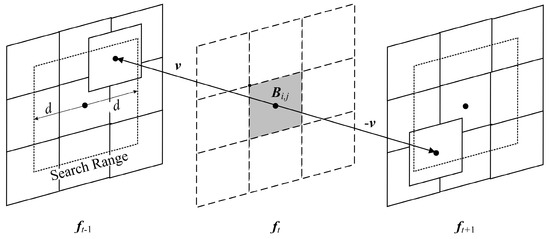
Figure 1.
Illustration on Bidirectional Motion Estimation (BME).
When using FS, the search range D in ft−1 and ft+1 is confined to a displacement ±d around the aligned pixel to the center of Bi, and the candidate MV set V is constructed by scanning all of the search points in D. The Sum of Bidirectional Absolute Differences (SBAD) is used as block matching criterion to evaluate the reliability of each MV candidate, i.e.,
where ft−1(s) and ft+1(s) represent the luminance values of the pixel s in ft−1 and ft+1. The SBADs of all candidate MVs are computed, and then the best MV vi,j for Bi,j by minimizing SBAD, i.e.,
BME requires (2d + 1)2 SBAD operations to locate the matching block for each absent block, and there are many redundant SBAD operations due to the local smoothness of MVF. Besides, BME shows its inefficiency in the texture regions, because the temporal symmetry is disturbed by the repeated similar structures. We can speed up BME by subsampling and predictive search. The texture details are removed when filtering video frames by low-pass filter before subsampling, which suppresses the bad effects that result from repeated similar structures. However, it is important for BME to have the edge details in order to ensure high accuracy, so we should use EPF to preserve edges while removing textures. The following part briefly introduces EPF.
2.2. Edge-Preserved Filtering (EPF)
EPF is an important image filtering technology that smoothes away textures while also retaining sharp edges, and it has been widely applied to detail manipulation, tone mapping, pencil drawing, and so on. EPF has gained a lot of attention over the last two decades, in which the most popular filters in EPF are bilateral filter [25], guided filter [26], and anisotropic diffusion [30]. Anisotropic diffusion is implemented with lots of iterations, and bilateral and guided filters compute a space-varying weight at a space of higher dimensionality than that of the signal being filtered. Therefore, these popular filters have high computational complexity. Many techniques have been proposed to speed up EPF, among which the best known is Recursive Filter based on Domain Transform (RFDT) [31]. RFDT is sufficiently fast for real-time performance, e.g., one-megapixel color images can be filtered in 0.007 s on a GPU. Therefore, we use RFDT to filter each video frame in our FRUC algorithm.
The idea of RFDT is to reduce the dimensionality of image before filtering. In a five-dimensional space, EPF can be defined as a space-invariant kernel whose response decreases with distance. If this kernel preserves the original distances at a five-dimensional space, it would also maintain the edge-preserving property in a lower dimensional space. RFDT transforms the input image I into the transformed domain Ωw by
in which ct(·) represents the domain transform operator, δs and δr is the spatial and range standard deviation, respectively. Suppose that L is the transformed signal of I by the operator ct(·), and it is processed, as follows:
where a∈[0, 1] is a feedback coefficient, L[m] represents the m-th value in L, L[m] = ct(xm), xm is the m-th value in I, J[m] is the m-th value of filtered result J, and d = ct(xm) − ct(xm−1) is the distance in Ωw between the neighboring samples xm and xm−1. As d increases, ad approaches to zero, converging Equation (6), which results in similar values of the pixels at the same side of edge, and the pixels on different sides of edge have largely different values, thus preserving edges. As shown in Figure 2, it can be seen that, by using RFDT, the textures on the petals are efficiently suppressed, and the edges of petals are preserved, which indicated that RFDT is an efficient EPF, and it is helpful in improving the accuracy of BME.
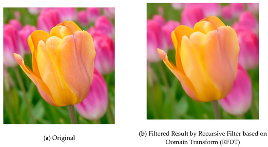
Figure 2.
Visual comparison between the original image and the filtered image by RFDT.
3. Proposed FRUC Algorithm
3.1. Framework Overview
Figure 3 presents the framework of the proposed FRUC algorithm. Each frame is first filtered by EPF to preserve edges while also suppressing the textures, and then subsampled to reduce the computational complexity. BME is performed on the subsampled frames and the predictive search is used to reduce the redundant search points according to the local smoothness of MVF. For BME, the forward ME is used to compute the MVF from the previous frame to the next frame, and the bidirectional refinement is used to refine the MVF of the interpolated frame based on the MVF output by forward ME. Finally, according to the refined MVF, the Overlapped Block Motion Compensation (OBMC) [32] is used to produce the interpolated frame. The following describes the EPF-based subsampling and BME with predictive search in detail.
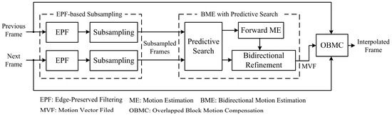
Figure 3.
Framework of the proposed Frame Rate Up-Conversion (FRUC) algorithm.
3.2. EPF-Based Subsampling
Before subsampling, we use EPF to filter out textures on object surface in a video frame. The implementation of EPF includes four steps to prevent the over-smoothing of object edges, in which the visual result after each step is illustrated in Figure 4. Suppose that f denotes the to-be-filtered frame, RFTD is first used to filter each frame, as follows:
in which δs and δr are used to control the amount of smoothing. We need to over-smooth the image to extract the edges and textures as many as possible. By testing several (δs, δr) pairs on the nature images, we find that the over-smoothing effects are appropriate when setting δs and δr to be 30 and 100. As shown in Figure 4a, we can see that, although the most of textures on surfaces are suppressed, the edges of objects are blurred. We extract the high-pass components by the following difference operator to enhance the edges:
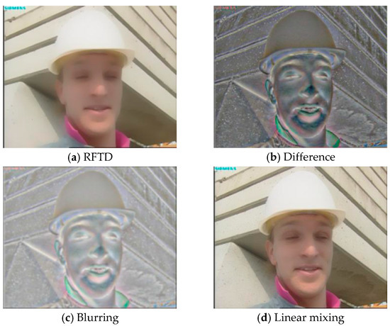
Figure 4.
Illustrations on the different steps of Edge-Preserved Filtering (EPF) for the second frame of Foreman sequence.
As shown in Figure 4b, the high-pass components include edges and textures, so we further suppress textures in high-pass components by the Gaussian blur, as follows:
in which GausBlur(·) represents the function of Gaussian blurring, w is the window size, and σ is the standard deviation. We should set a small w value and a big σ value due to the locally and rapidly varying statistics of textures. By several experiments, we find that the texture can be effectively suppressed when w and σ are, respectively, set to be 3 and 100. As shown in Figure 4c, the textures on object surfaces are mostly filtered out and the edges are retained. Finally, we linearly mix fGS into f, as follows:
As shown in Figure 4d, after linear mixing, the edges are enhanced and textures are efficiently suppressed. Figure 5 presents the visual results of EPF, average filtering, Gaussian filtering, and original frame for the second frame of Foreman sequence. It can be seen that severe blurs occur on the filtered frames by average filtering and Gaussian filtering, but EPF produces a clear result. When compared with the original frame, we can see that many textures are smoothed and edges have not been destroyed in the filtered frame by EPF. For computational complexity, the designed EPF can be implemented in O(MN) for a video frame, with the size of M×N, guaranteeing filtering in real time.
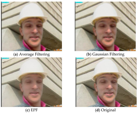
Figure 5.
Comparisons of the visual results of EPF, average filtering, Gaussian filtering, and original frame for the second frame of Foreman sequence.
3.3. BME with Predictive Search
Forward ME is first performed to provide the MVF Vt+1,t−1, from ft+1 to ft−1. The redundant search points are removed based on the local smoothness of MVF. For the i-th row and j-th column block in ft+1, as shown in Figure 6a, its candidate MV set is constructed by
in which Vt+1,t−1 and Vt−1,t−3 denote, respectively, the MVF from ft+1 to ft−1 and the MVF from ft−1 to ft−3, and denote, respectively, the i-th row and j-th column block in ft+1 and ft−1, Vt+1,t−1[] denotes the MV of in the MVF Vt+1,t−1, Vt−1,t−3[] denotes the MV of in the MVF Vt−1,t−3, and R1, R2 are two MV biases that are randomly selected from the set U. The best forward MV for is computed based on the Sum of Absolute Difference (SAD), as follows:
in which s denotes the pixel position in the block , ft+1(s) and ft−1(s), respectively, denote the pixel values at the position s in ft+1 and ft−1. According to the MVF output by forward ME, the bidirectional refinement is performed to assign a unique MV for each block in ft. First, we obtain the MVFs Vt+1,t and Vt−1,t−2,by
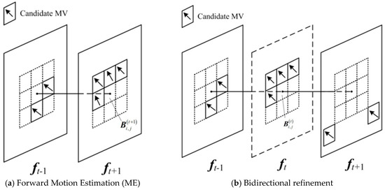
Figure 6.
Illustrations on candidate Motion Vectors (MVs) for forward ME and bidirectional refinement.
The local smoothness of MVF ensures that there is MV consistency in a spatio-temporal neighborhood, so we construct the candidate MV set for the i-th row and j-th column block in ft, as shown in Figure 6b, i.e.,
in which Vt,t−1, Vt−1,t−2, and Vt,t−1 denote, respectively, the MVF from ft to ft−1, the MVF from ft−1 to ft−2 and the MVF from ft to ft−1, Vt,t−1[] denotes the MV of in the MVF Vt,t−1, and R1, R2 are still randomly generated according to Equation (13). Afterwards, we compute the SBAD value for each candidate MV in and obtain the final MV for the absent block by
Several SAD and SBAD operators can be implemented when computing the MV for each block. BME has a low computation complexity due to the limited number of candidate MV set. Suppose that the size of a video frame is M × N, the implementation of BME in O(MN) time is straightforward.
4. Experimental Results
In this section, the performance of the proposed FRUC algorithm is evaluated by testing it on test sequences with CIF, 720P, and 1080P formats. The CIF sequences include foreman and football, the 720P sequences include ducks_take_off, in_to_tree, and old_town_cross, and the 1080P sequences include station2, speed_bag and pedestrian_area. These test sequences are downloaded on the website: https://media.xiph.org/video/derf/. The interpolated results by the proposed algorithm are compared with those that are generated by the traditional FRUC algorithms, including BME [13], EBME [14], and DS-ME [15]. We also compare the proposed algorithm with two recent FRUC algorithms [1,4] on some CIF sequences. We remove the first 50 even frames of each test sequence to evaluate the qualities of the interpolated frames from subjective and objective perspectives, and then use different FRUC algorithms to generate these even frames from the first 51 odd frames. In all of the algorithms, the block size B is, respectively, set to be 16, 32, and 64 for CIF, 720P, and 1080P formats, and the comparing algorithms keep their original parameter settings, except the block size. Peak Signal-to-Noise Ratio (PSNR) and Structural SIMilarity (SSIM) [33] between the interpolated frame and the original frame are used t undertake the objective evaluation. SSIM is a perceptual metric that is based on visible structure, and it is closer to human perception than PSNR. The computational complexity is evaluated by the execution time. All of the experiments are conducted on a Windows machine with an Intel Core i7 3.40 GHz CPU and a memory of 8 GB. All of the algorithms are implemented in MATLAB.
4.1. Effects of Subsampling
In this subsection, we discuss the effects of various subsampling schemes on the qualities of interpolated frames. Table 1 shows the average PSNR values of all the test sequences recovered by the proposed FRUC algorithm when using different subsampling schemes, including non-subsampling, average filtering, Gaussian filtering, and EPF. For non-subsampling, each frame is directly input into ME without being subsampled. The non-subsampling has obvious PSNR gains when compared with other schemes because none of the details are discarded, but it costs more computation. Before subsampling, the average filter and Gaussian filter are performed on each frame, and they have similar PSNR losses as compared with the non-subsampling when the subsampling factor is respectively set to be 2, 4, and 8. The PSNR losses result from the destruction of high-frequency components. When performing EPF, the PSNR losses are alleviated, especially when setting a big subsampling factor, e.g., when the subsampling factor is 8, the PSNR loss of EPF is obviously less than those of average and Gaussian filtering. Therefore, it can be observed that the suppression of texture details helps to improve the ME accuracy.

Table 1.
Average PSNRs (dB) of test sequences recovered by the proposed FRUC algorithm with different subsampling schemes.
4.2. Objective Evaluation
Table 2 presents the average PSNR values, SSIM values, and execution time of test sequences recovered by various FRUC algorithms. For the proposed algorithm, the subsampling factor is set to be 2. First, we analyze the average PSNR values of various FRUC algorithms. For the sequences with stable and low-speed motions, the PSNR values of the proposed algorithm are comparable with those of the traditional methods, e.g., for the ducks_take_off sequence, the PSNR loss is about 0.25 dB when compared with the traditional algorithms. For the sequences with complex and high-speed motions, the PSNR losses of the proposed algorithm moderately increase, e.g., for old_town_cross sequence, when compared with DS-ME, the PSNR loss is 1.65 dB. All of the sequences considered, the average PSNR value of the proposed algorithm is 31.35 dB, and the largest PSNR loss is 1.43 dB when compared with all traditional algorithms. Second, we analyze the average SSIM values of different FRUC algorithms. Similar to PSNR results, the proposed algorithm has comparable SSIM values with traditional algorithms for the sequences with stable and low-speed motions, and it has moderate losses for the sequences with complex and high-speed motions. All of the sequences considered, the average SSIM value of the proposed algorithm is 0.9005, and the largest SSIM loss is 0.0209 when compared with all traditional algorithms. By PSNR and SSIM comparisons, we can see that our algorithm has an advantage in quality degradation over the traditional algorithms. Finally, we analyze the average execution time of various FRUC algorithms. For CIF sequences, it takes BME, EBME, and DS-ME about 1–2 s to interpolate a frame, but the proposed algorithm only about 0.2 s. For 720P sequences, the proposed algorithm spends approximately 0.7 s in interpolating a frame, and the comparing algorithms about 9–35 s. For 1080P sequences, the comparing algorithms use about 222 s at most and 23 s at least, while the proposed algorithm only about 1.6 s to interpolate a frame. All of the sequences considered, the proposed algorithm only needs an average of 0.95 s per frame, and its execution time is far less than that of the comparing algorithms. With PSNR, SSIM, and execution time all taken into consideration, it can be seen that the proposed algorithm does not have a large PSNR loss while maintaining its time advantage. Therefore, we come to the conclusion that it can provide a good objective quality with a low computation complexity.
Table 2.
Average Peak Signal-to-Noise Ratios (PSNRs) (dB), Structural SIMilarities (SSIMs), and execution time (second per frame) of test sequences recovered by various FRUC algorithms.
Table 3 presents the PSNR results of the proposed algorithm and two recent FRUC algorithms [1,4]. The results of [1,4] are directly taken from their originals. When compared with [1], our algorithm has 1.25 dB PSNR gain only for container sequence, and it has some PSNR losses for other sequences. Ref. [1] uses more advanced tools to construct the interpolation model, and it improves the objective qualities of interpolated frames at any computational cost. However, our algorithm aims to simplify the interpolation model, so its improvement of interpolation quality is limited. It has similar PSNR values to those of [4], whose core is Support Vector Machine (SVM), which is trained with lots of data and computation. In a word, our algorithm consumes less computation to obtain comparable results to [4].
Table 3.
Average PSNRs (dB) comparison of the proposed algorithm and two recent FRUC algorithms [1,4].
4.3. Subjective Evaluation
Figure 7 presents the visual results on the 78th interpolated frame of foreman sequence while using different FRUC algorithms. The displacement of nose and eyes occurs on the 78th frame of foreman sequence due to the moving head, as shown in the red rectangle of Figure 7a. BME in Figure 7b cannot effectively track the moving head, and thus results in severe ghost effects. EBME in Figure 7c produces a misplaced nose, and DS-ME in Figure 7d generates severe blocking artifacts. As shown in Figure 7d, the proposed algorithm produces a better visual result than other algorithms, and it effectively suppresses the blocking artifacts. Figure 8 presents the visual results on the 78th interpolated frame of in_to_tree sequence while using different FRUC algorithms. As shown in Figure 8a, there are some repeated windows in the red rectangle, and the occlusion occurs due to the transition of cameras. BME in Figure 8b and EBME in Figure 8c produce several incomplete windows. Severe ghost effects occur around windows for DS-ME in Figure 8d. The proposed algorithm in Figure 8e produces a comparable visual result to the truth ground. Figure 9 presents the visual results on the fourth interpolated frame of speed_bag sequence while using different FRUC algorithms. As shown in Figure 9b,c, BME and our algorithm generate ghost effects around the head of sportsman. EBME in Figure 9c and DS-ME in Figure 9d produce severe blocking artifacts. Especially in the red rectangle of Figure 9a, the proposed algorithm can clearly recover these letters while other algorithms would generate some blurring and blocking artifacts. From the above results, it can be concluded that the proposed algorithm can bring good subjective quality.
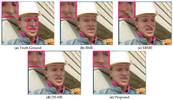
Figure 7.
Visual results on the 78th interpolated frame of foreman sequence while using different FRUC algorithms.
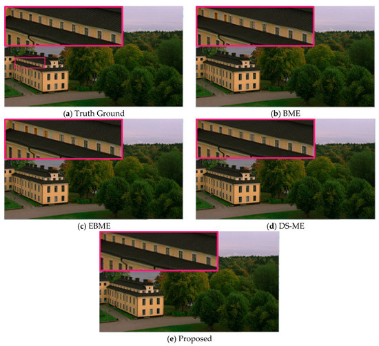
Figure 8.
Visual results on the 78th interpolated frame of in_to_tree sequence using different FRUC algorithms.
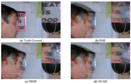
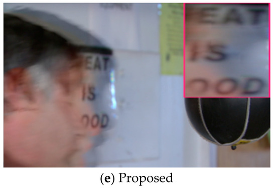
Figure 9.
Visual results on the 4th interpolated frame of speed_bag sequence using different FRUC algorithms.
5. Conclusions
In this paper, we present a low-complex FRUC using EPF-based subsampling and BME with predictive search. Each frame is first filtered by EPF to preserve the edge details and suppress texture details, and it is then subsampled to reduce the computational complexity. The subsampled frames are input into BME to generate the MVFs of the interpolated frames. The predictive search is used to speed up BME, and several spatially and temporally neighboring MVs are selected as candidates, according to the local smoothness of MVF. The experimental results show that the proposed FRUC algorithm brings good objective and subjective qualities of the up-converted video sequences, while also reducing the computational complexity.
Author Contributions
R.L. contributed to the concept of the research, performed the data analysis and wrote the manuscript; W.M. helped perform the data analysis with constructive discussions and helped performed the experiment. Y.L. and L.Y. revised the manuscript, and provided the necessary support for the research. All authors have read and agreed to the published version of the manuscript.
Funding
This work was supported in part by the National Natural Science Foundation of China, under Grant nos. 31872704, 61572417, in part by Innovation Team Support Plan of University Science and Technology of Henan Province (No. 19IRTSTHN014).
Conflicts of Interest
The authors declare no conflict of interest.
References
- Bao, W.; Zhang, X.; Chen, L.; Ding, L.; Gao, Z. High-Order Model and Dynamic Filtering for Frame Rate Up-Conversion. IEEE Trans. Image Process. 2018, 27, 3813–3826. [Google Scholar] [CrossRef]
- Dar, Y.; Bruckstein, A.M. Motion-compensated coding and frame rate up-conversion: Models and analysis. IEEE Trans. Image Process. 2015, 24, 2051–2206. [Google Scholar] [CrossRef]
- Huang, Y.L.; Chen, F.C.; Chien, S.Y. Algorithm and architecture design of multi-rate frame rate up-conversion for ultra-HDLCD systems. IEEE Trans. Circuits Syst. Video Technol. 2017, 27, 2739–2752. [Google Scholar] [CrossRef]
- Van, X.H. Statistical search range adaptation solution for effective frame rate up-conversion. IET Image Process. 2018, 12, 113–120. [Google Scholar]
- Choi, D.; Song, W.; Choi, H.; Kim, T. MAP-Based Motion Refinement Algorithm for Block-Based Motion-Compensated Frame Interpolation. IEEE Trans. Circuits Syst. Video Technol. 2016, 26, 1789–1804. [Google Scholar] [CrossRef]
- Van Thang, N.; Choi, J.; Hong, J.H.; Kim, J.S.; Lee, H.J. Hierarchical Motion Estimation for Small Objects in Frame-Rate Up-Conversion. IEEE Access 2018, 6, 60353–60360. [Google Scholar] [CrossRef]
- Gao, X.Q.; Duanmu, C.J.; Zou, C.R. A multilevel successive elimination algorithm for block matching motion estimation. IEEE Trans. Image Process. 2000, 9, 501–504. [Google Scholar] [CrossRef]
- De Haan, G.; Biezen, P.W.A.C.; Huijgen, H.; Ojo, O.A. True-motion estimation with 3-D recursive search block matching. IEEE Trans. Circuits Syst. Video Technol. 1993, 3, 368–379. [Google Scholar] [CrossRef]
- Dikbas, S.; Altunbasak, Y. Novel true-motion estimation algorithm and its application to motion-compensated temporal frame interpolation. IEEE Trans. Image Process. 2012, 22, 2931–2945. [Google Scholar] [CrossRef]
- Cetin, M.; Hamzaoglu, I. An adaptive true motion estimation algorithm for frame rate conversion of high definition video and its hardware implementations. IEEE Trans. Consum. Electron. 2011, 57, 923–931. [Google Scholar] [CrossRef]
- Tai, S.C.; Chen, Y.R.; Huang, Z.B.; Wang, C.C. A multi-pass true motion estimation scheme with motion vector propagation for frame rate up-conversion applications. J. Disp. Technol. 2008, 4, 188–197. [Google Scholar]
- Tsai, T.H.; Lin, H.Y. High visual quality particle based frame rate up conversion with acceleration assisted motion trajectory calibration. J. Disp. Technol. 2012, 8, 341–351. [Google Scholar] [CrossRef]
- Choi, B.T.; Lee, S.H.; Ko, S.J. New frame rate up-conversion using bi-directional motion estimation. IEEE Trans. Consum. Electron. 2000, 46, 603–609. [Google Scholar] [CrossRef]
- Kang, S.J.; Cho, K.R.; Kim, Y.H. Motion compensated frame rate up-conversion using extended bilateral motion estimation. IEEE Trans. Consum. Electron. 2007, 53, 1759–1767. [Google Scholar] [CrossRef]
- Yoo, D.G.; Kang, S.J.; Kim, Y.H. Direction-select motion estimation for motion-compensated frame rate up-conversion. J. Disp. Technol. 2013, 9, 840–850. [Google Scholar]
- Ferroukhi, M.; Ouahabi, A.; Attari, M.; Habchi, Y.; Taleb-Ahmed, A. Medical video coding based on 2nd-generation wavelets: Performance evaluation. Electronics 2019, 8, 88. [Google Scholar] [CrossRef]
- Chen, Z.; He, T.; Jin, X.; Wu, F. Learning for video compression. IEEE Trans. Circuits Syst. Video Technol. 2019. [Google Scholar] [CrossRef]
- Ouahabi, A. SIGNAL and Image Multiresolution Analysis; ISTE-Wiley: London, UK, 2012. [Google Scholar]
- Kappeler, A.; Yoo, S.; Dai, Q.; Katsaggelos, A.K. Video super-resolution with convolutional neural networks. IEEE Trans. Comput. Imaging 2016, 2, 109–122. [Google Scholar] [CrossRef]
- Sidahmed, S.; Messali, Z.; Ouahabi, A.; Trépout, S.; Messaoudi, C.; Marco, S. Nonparametric denoising methods based on contourlet transform with sharp frequency localization: Application to electron microscopy images with low exposure time. Entropy 2015, 17, 2781–2799. [Google Scholar]
- Ouahabi, A. A review of wavelet denoising in medical imaging. In Proceedings of the 8th IEEE International Workshop on Systems, Signal Processing and Their Applications (WoSSPA), Algiers, Algeria, 12–15 May 2013; pp. 19–26. [Google Scholar]
- Sivanantham, S. High-throughput deblocking filter architecture using quad parallel edge filter for H. 264 video coding systems. IEEE Access 2019, 7, 99642–99650. [Google Scholar]
- Bao, W.; Lai, W.S.; Zhang, X.; Gao, Z.; Yang, M.H. MEMC-Net: Motion estimation and motion compensation friven neural network for video interpolation and enhancement. IEEE Trans. Pattern Anal. Mach. Intell. 2019. [Google Scholar] [CrossRef] [PubMed]
- Rüfenacht, D.; Taubman, D. HEVC-EPIC: Fast optical flow estimation from coded video via edge-preserving interpolation. IEEE Trans. Image Process. 2018, 27, 3100–3113. [Google Scholar] [CrossRef] [PubMed]
- Durand, F.; Dorsey, J. Fast bilateral filtering for the display of high-dynamic-range images. ACM Trans. Graph. 2002, 21, 257–266. [Google Scholar] [CrossRef]
- He, K.; Sun, J.; Tang, X. Guided image filtering. IEEE Trans. Pattern Anal. Mach. Intell. 2012, 35, 1397–1409. [Google Scholar] [CrossRef] [PubMed]
- Yoon, S.J.; Kim, H.H.; Kim, M. Hierarchical Extended Bilateral Motion Estimation-Based Frame Rate Upconversion Using Learning-Based Linear Mapping. IEEE Trans. Image Process. 2018, 27, 5918–5932. [Google Scholar] [CrossRef] [PubMed]
- He, J.; Yang, G.; Song, J.; Ding, X.; Li, R. Hierarchical prediction-based motion vector refinement for video frame-rate up-conversion. J. Real-Time Image Process. 2018, 1–15. [Google Scholar] [CrossRef]
- Nam, K.M.; Kim, J.S.; Park, R.H.; Shim, Y.S. A fast hierarchical motion vector estimation algorithm using mean pyramid. IEEE Trans. Circuits Syst. Video Technol. 1995, 5, 344–351. [Google Scholar]
- Perona, P.; Malik, J. Scale-space and edge detection using anisotropic diffusion. IEEE Trans. Pattern Anal. Mach. Intell. 1990, 12, 629–639. [Google Scholar] [CrossRef]
- Gastal, E.S.L.; Oliveira, M.M. Domain transform for edge-aware image and video processing. ACM Trans. Graph. (ToG) 2011, 30, 69. [Google Scholar] [CrossRef]
- Orchard, M.T.; Sullivan, G.J. Overlapped block motion compensation: An estimation-theoretic approach. IEEE Trans. Image Process. 1994, 3, 693–699. [Google Scholar] [CrossRef]
- Wang, Z.; Bovik, A.C.; Sheikh, H.R.; Simoncelli, E.P. Image quality assessment: From error visibility to structural similarity. IEEE Trans. Image Process. 2004, 13, 600–612. [Google Scholar] [CrossRef] [PubMed]
© 2020 by the authors. Licensee MDPI, Basel, Switzerland. This article is an open access article distributed under the terms and conditions of the Creative Commons Attribution (CC BY) license (http://creativecommons.org/licenses/by/4.0/).