Novel Prediction Framework for Path Delay Variation Based on Learning Method

Abstract

Path delay variation becomes a serious concern in advanced technology, especially for multi-corner conditions. Plenty of timing analysis methods have been proposed to solve the issue of path delay variation, but they mainly focus on every single corner and are based on a characterized timing library, which neglects the correlation among multiple corners, resulting in a high characterization effort for all required corners. Here, a novel prediction framework is proposed for path delay variation by employing a learning-based method using back propagation (BP) regression. It can be used to solve the issue of path delay variation prediction under a single corner. Moreover, for multi-corner conditions, the proposed framework can be further expanded to predict corners that are not included in the training set. Experimental results show that the proposed model outperforms the traditional Advanced On-Chip Variation (AOCV) method with 1.4X improvement for the prediction of path delay variation for single corners. Additionally, while predicting new corners, the maximum error is 4.59%, which is less than current state-of-the-art works.

1. Introduction

Variation is a significant and expensive problem. Accompanying the development of integrated circuits, the feature size of technology is getting smaller and smaller and will continue shrinking in the future. However, the size of atoms does not change. Regarding advanced technology, the oxide layer of the gate is just a few atoms thick, so even a single atom out of place can change device and cell performance considerably [1]. As the voltage decreases, the dependence of the transistor current on threshold (Vth), supply voltage (Vdd) and temperature gradually changes from linear to exponential [2,3,4,5,6]. The gate delay variation increases by five times in near-threshold voltage [7] and two times across the entire temperature [8]. Moreover, considering modern technology, due to the complexity and variability of semiconductor processes, delay variation is no longer a simple relationship of the process, voltage, and temperature (PVT), so sensitivity of delay variation varies differently [9,10]. Therefore, the worst corner of different designs may be different and cannot be easily identified. Every corner needs to be analyzed, and corner numbers have increased by 1000 at 32 nm [11,12,13]. Besides, the characterizations and simulations of each corner are very long, so much time and effort are needed to verify circuit functionality in all kinds of corners. Also, low voltage has a dramatic influence on path delay variation because, at low voltage, delay variation does not obey Gaussian distribution but non-Gaussian distribution [14,15,16,17,18,19,20], which makes the path delay variation more difficult to predict.

Considering variation, various techniques are proposed, such as post-silicon tuning techniques [21,22], but they are the tuning techniques that cannot be used as the analysis in advance. SPICE Monte Carlo (MC) is considered an accurate method for variation analysis, however, it needs extremely large computational effort and is impractical for large designs. Statistical Static Timing Analysis (SSTA) [23,24,25] was developed about ten years ago and was based on Gaussian gate delay distribution. However, it requires too much run time and memory and has not been widely used in the industry. Then, the On-Chip Variation (OCV) and the Advanced OCV (AOCV) [26] were introduced in the current timing analysis flow and provide sufficient accuracy and risk reduction for Integrated Circuits (IC) designs, but they compare similarly to traditional best-case and worst-case methods, which means they are all corner-based methodology. They can only obtain the path delay variation on the given characterized corners. However, in reality, many un-characterized corners need to be analysed to improve the accuracy of the designs. During such situations, it must take time to characterize the timing library, but the number of signoff corners increases to hundreds or thousands which makes the characterization effort increase too dramatically to withstand. Therefore, it is difficult to trade-off between precision and overhead of the characterizing library. To save characteristic effort and predict path delay variation at multi-corner conditions, many researchers have studied it [16,27]. Alioto et al. [27] regard the delay independent of temperature and voltage at the reference of Fonout of Four (FO4) and it provides a relatively high accuracy and avoids heavy characterization effort. Rithe’s et al. [16] method needs less effort to characterize a cell at one corner but cannot predict the timing at a new corner.

Recently, the learning-based method has been widely used in all kinds of fields [28,29,30], such as optical, image processing and also the Electronics Design Automation (EDA) field, especially timing analysis, and has shown great potential [31,32,33]. Das et al. [31] build a model that still focuses the cell delay model by a learning-based method that comprehensively captures process, voltage, and temperature, along with input slew and output load, but it is not suited for path delay variation prediction directly. Kahng et al. [32] use a machine learning method to solve the signal integrity (SI) timing problems, which is based on the timing reports from the non-SI mode. It is robust across designs and signoff constraints. Han et al. [33] apply a learning-based method to solve the correlation problem of different timing signoff tools. They develop a learning-based tool to correct the divergence of all kinds of delays at different tools. The applications mentioned all use a learning-based method to solve the timing related issue, which demonstrates the learning method is a promising method to solve the timing prediction problem.

Here, we introduce a novel prediction framework for path delay considering local variation. The framework uses a learning-based method, first to obtain the relationship of the delay variation with circuit features at some corners and, second, to predict new path delay variation at a single corner and unknown corner delay variations at multi-corners. The contributions of the paper are as follows:

• Regarding the single corner, it not only eliminates the characterization effort for the timing library of each cell, but also performs better than AOCV.
• Concerning the multi-corner, the single model setting can be easily expanded to multi-corner, which is not possible in traditional AOCV and MC methods and have less error compared to existing works.

The structure of the paper is as follows: Section 2 introduces the proposed prediction framework for path delay variation based on Machine Learning (ML) from single corner and multi-corner condition perspectives. The experimental setting and results discussion are presented in Section 3. Section 4 concludes this work.

2. Proposed Prediction Framework for Path Delay Variation-Based Learning Method

Concerning practical designs, the severe timing constraint is required to satisfy the desired performance. To meet the clock constraint, the prediction of path delay variation is a crucial issue.

A learning-based framework is proposed for the delay variation prediction of a circuit path, without the requirement of corner-based timing libraries, which is illustrated in Figure 1. The first step is data preparation, which mainly contains the generation of train paths. Then, path delay/delay variation can be obtained by fast SPICE nominal/MC simulation. The basic path features are extracted based on the prepared paths, which are divided into single corner and multi-corner and will be presented in Section 2.2. The last step is the network configuration. The Back Propagation (BP) network [34,35] is selected to build the model due to the problem of regression. The weights and thresholds of every layer and the junction points of the network are acquired through iterations for the train set. The network layers and junction points are adjusted, and the effective features are reselected until the result meets its convergence. The main core steps are training set preparation, features selection and network configuration in the learning-based method.

2.1. Data Preparation

The first issue faced by the learning-based method is how to construct the training set. Based on the above analysis, the problem we focus on is the path delay variation. To improve the coverage of the training set samples for different circuit parameters and limit the number of MC simulations required for the training set, a group of artificial paths with multiple random gates, sizes, load capacitances, and stages is generated. Meanwhile, the following assumptions are needed during the generation of artificial paths.

(1) All path branches are removed by being replaced with given values for load capacitance.

(2) All values of float input ports of multi-input gates are assumed to be 1 or 0 to ensure it does not influence the signal propagation. Taking the NAND2 gate as an example, one input connects the previous output, and the other input is set to 1.

Under the assumptions mentioned above, all path delay without/with any local variations is measured by SPICE/fast MC simulation based on the generated paths.

2.2. Feature Selection

Effective feature selection is another critical step for the learning-based method. The selected features are introduced in the following.

Since the problem of this paper is the regression problem of supervised learning, the input and output features are necessary. The features contain cell topology features, a path delay feature and corner conditions, whose detailed definitions are listed in

Table 1. Feature selection and notation.

Category	Feature	Notation	Single Corner	Multi-Corner
cell	size	the drive strength of each gate	√	√
	Nstack	the stack transistor number of each gate	√	√
path	polar	rise of fall of each gate	√	√
	load	the load capacitance of each stage	√	√
	td	the nominal delay of each path	√	√
	$t{d}_{x\sigma }$	the variation delay of each path at xσ	√	√
corner	T	the temperature of the operation condition	-	√
	V	the voltage of the operation condition	-	√

. The $t{d}_{x\sigma }$ is the output feature, and the others are input features.

Size and N_stack constitute cell topology. Size refers to the width of the transistor, that is, the driving strength of the gate, such as X1, X2 and so on. N_stack indicates the stack transistors number of the gate. Random variations across different stacked transistors tend to average out and reduce the variability, compared to a single transistor by the square of N_stack. Therefore, the N_stack is an effective feature of the BP network. A gate has a different N_stack, however, based on the charging and discharging. Taking NAND2 as an example, the N_stack is 2 when discharging, and 1 while charging.

Thus, in a real path, another feature that needs to be introduced is called polar. Polar means representing the transition direction of a gate which is charging or discharging, and it can be obtained according to the propagation characteristics of each gate in the path. The load of each stage and path delay (td) can be easily obtained in the data preparation phase.

Temperature (T) and voltage (V) are the two features that are different from the single-corner and multi-corner conditions. Seen in the single corner prediction the two features are not included, but, in the multi-corner prediction they need to be added.

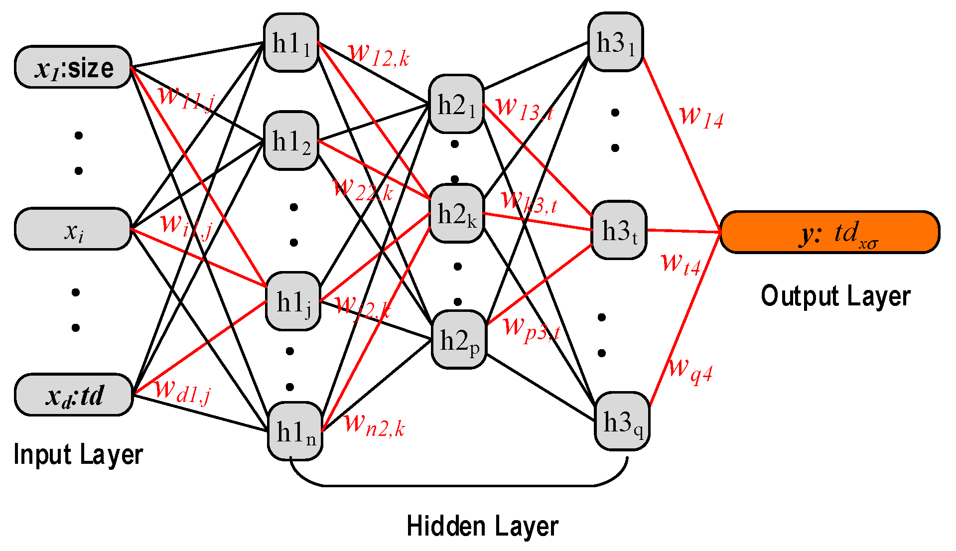
2.3. Network and Configuration

The variation delay of a path can be expressed as follows:

$$t{d}_{x\sigma }=F\left(size,N_{stack},polar,load,td,T,V\right)$$

Concerning a single corner, the feature of T and V can be ignored, but for multi-corners, the T and V are necessary. F is a complex and continuous function. Due to the path delay variation prediction belong to the regression problem, the BP neural network is adopted. The architecture of BP, with three hidden layers, is illustrated in Figure 2, which contains input, hidden and output layers. The input layer concludes the features mentioned in Section 2.2, and the output layer is the path delay variation value. We assume the input layer has d neurons (x1, …, xi, …, xd), the hidden layers has n (h1₁, h1₂, …, h1_j, …, h1_n), p (h2₁, …, h2_k, …, h2_p), q (h3₁, …, h3_t, …, h2_q) neurons respectively, and the output layers has l neurons (y). and every active function are all sigmoid, the weights and biases are expressed by w and b. Additionally, every neuron input and output function is listed in

Table 2. Input and Output function of every layer.

	Function
	Input	Output
Hidden 1 layer	$ne{t}_{h{1}_j}={\displaystyle \sum _{i=1}^d{w}_{i1,j}{x}_i}+b_0$	$ou{t}_{h{1}_j}=\frac{1}{1+e^{-ne{t}_{h{1}_j}}}$
Hidden 2 layer	$ne{t}_{h{2}_k}={\displaystyle \sum _{j=1}^n{w}_{j2,k}ou{t}_{h{1}_j}}+b_1$	$ou{t}_{h{2}_k}=\frac{1}{1+e^{-ne{t}_{h{2}_k}}}$
Hidden 3 layer	$ne{t}_{h{3}_t}={\displaystyle \sum _{k=1}^p{w}_{k3,t}ou{t}_{h{2}_k}}+b_2$	$ou{t}_{h3}{}_{{}_t}=\frac{1}{1+e^{-ne{t}_{h{3}_t}}}$
Output layer	$ne{t}_y={\displaystyle \sum _{t=1}^q{w}_{t3}ou{t}_{h{3}_t}}+b_3$	$ou{t}_y=\frac{1}{1+e^{-ne{t}_y}}$

, where the net and out denote the input and output function of the neuron. It computes the result of every neuron by a forward propagation network and adjusts weights, biases, the number of layers and junction points by back propagation to minimize the total errors of all neurons during the network building.

3. Experimental Results and Discussions

Experiments were carried out under the process of Semiconductor Manufactory International Corporation (SMIC) 40 nm. Considering training and testing, plenty of paths were generated with randomly chosen cells and connecting structure, as described in Section 2. The path delay variation was characterized by 1% and 99% quantile with MC simulation for 1000 times. Regarding the training set, we chose a wide range of temperatures (0–25 °C) and voltages (0.6–1.1 V) to provide a reliable reference boundary which met the need of practical use for the model. The results of the predicting ability of the model are described through the mean relative error of the testing set, which is defined as follows:

$$error=\frac{1}{n}{\displaystyle {\sum }_1^n\left|\frac{y_i-{\stackrel{⌢}{y}}_i}{y_i}\right|}$$

where $y_i$ is the actual path delay variation value, and ${\stackrel{⌢}{y}}_i$ is the predicted value.

3.1. Path Delay Variation Prediction at a Single Corner

Path delay variation prediction at a single corner means that different models are built at each corresponding corner. Taking 5 stage path as an example, a detailed analysis of the training sample number and path delay accuracy are described in the following.

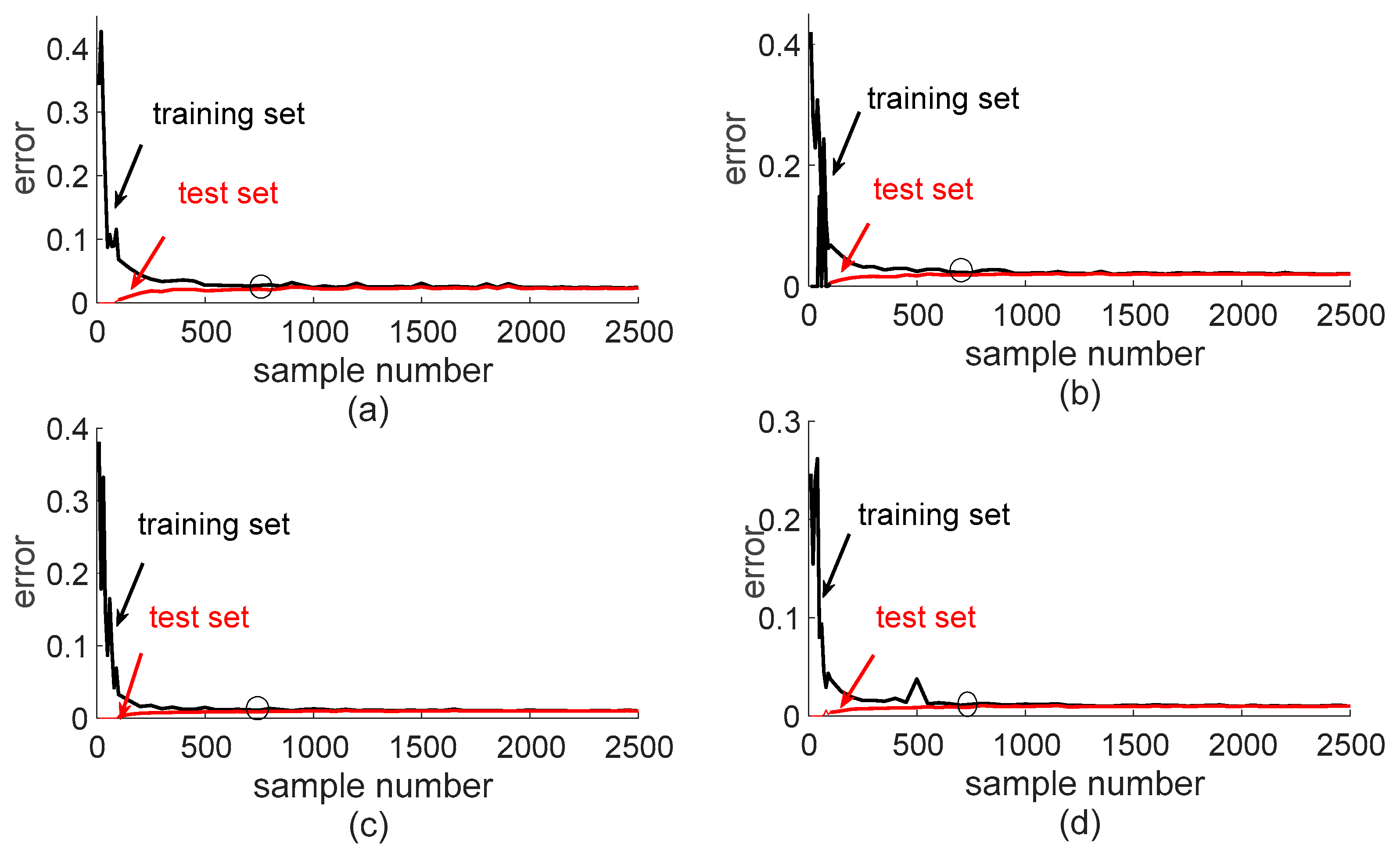
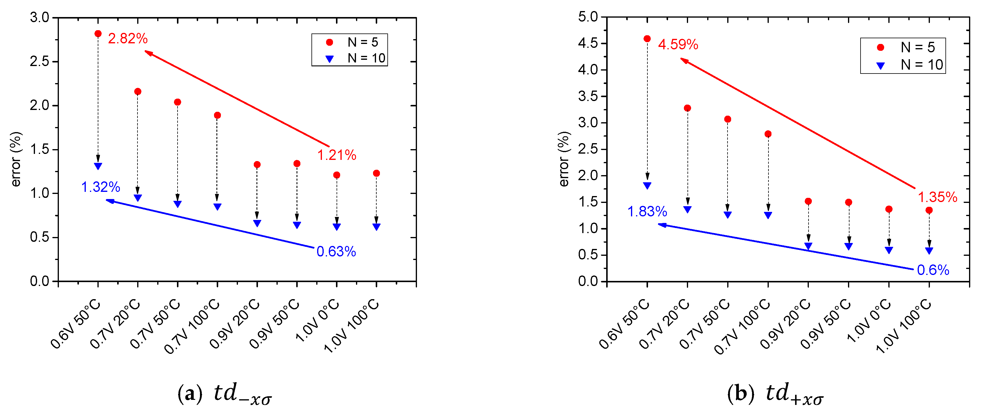
3.1.1. The Selection of Sample Number

It is commonly known that the more training data the network has, the higher the accuracy it will get. Enormous training data will have a more prominent cost, however. Looking at the training set, $t{d}_{-x\sigma }$ and $t{d}_{+x\sigma },$ every path is acquired by executing 1000 times MC simulations, on the one hand,, while, on the other hand, a larger training set will need more iterations to reach convergence for the network, which means more training time. Therefore, the trade-off between training sampling numbers and accuracy should be considered.

To attain the appropriate sample numbers for training, the analysis of the testing error curve with the number of training samples was adopted. To ensure the training sample number for our network, a large scope of training sample numbers was chosen, from 10 to 2500 with a step of 10. Figure 3 shows the x-axis indicates the training number, and the average error of the testing set (black line) and training set (red line) at this training sample is shown in the y-axis. Moreover, the curves are portrayed in several corners. We observed that for different corners, after 800 training samples, the testing error would decrease very slowly and this value was very close within different corners. Thus, we chose 700 as the number of training samples and 100 as the validation samples for saving SPICE simulation time and network training time in the context of guaranteed precision.

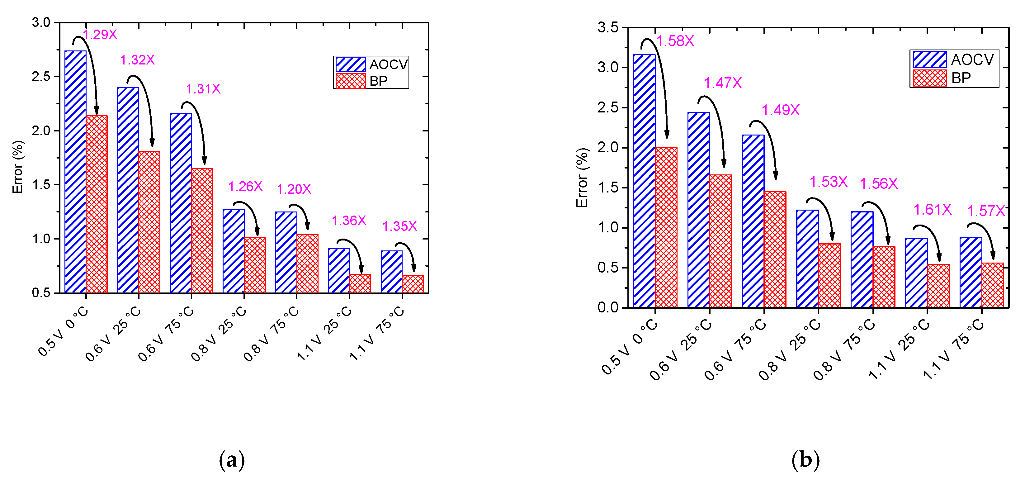
3.1.2. Path Delay Variation Prediction at Single Corner

The errors of the path variation delay across the two methods are illustrated in Figure 4 and Figure 5. One is the traditional method (AOCV), which predicts the worst case of the path delay variation by summarizing the nominal delays of all cells in the path with a derating coefficient for each stage. The other is the proposed method (BP-based), which predicts the delay of a new path by a network established by the training set. The x-axis represents the different operation conditions combined with all kinds of voltage and temperature, and the y-axis represents the mean error of the different methods.

Viewing the Figures, we can see that no matter if the probability is td_−xσ or td_+xσ, and no matter if the error is the train set or test set, the BP model performs better than AOCV. Regarding td_−xσ, the error in BP decreases by 1.20X–1.36X less than AOCV for the train set, and by 1.47X–1.58X for the test set. Concerning td_+xσ, the error in BP decreases by 1.43X–1.67X less than AOCV for the train set, and by 1.10X–1.49X for the test set. Therefore, it decreases by 1.4X on average. Besides, as the voltage decreases, the mean errors of the two methods are increasing, which is due to the non-gaussian distribution at low voltage. However, compared with AOCV, the error of the BP model increases more slowly, due to the network build of the BP model containing a complex non-linear operation base on the non-linear active function, which further demonstrates that BP is a more suitable method for the path delay variation prediction at low voltage.

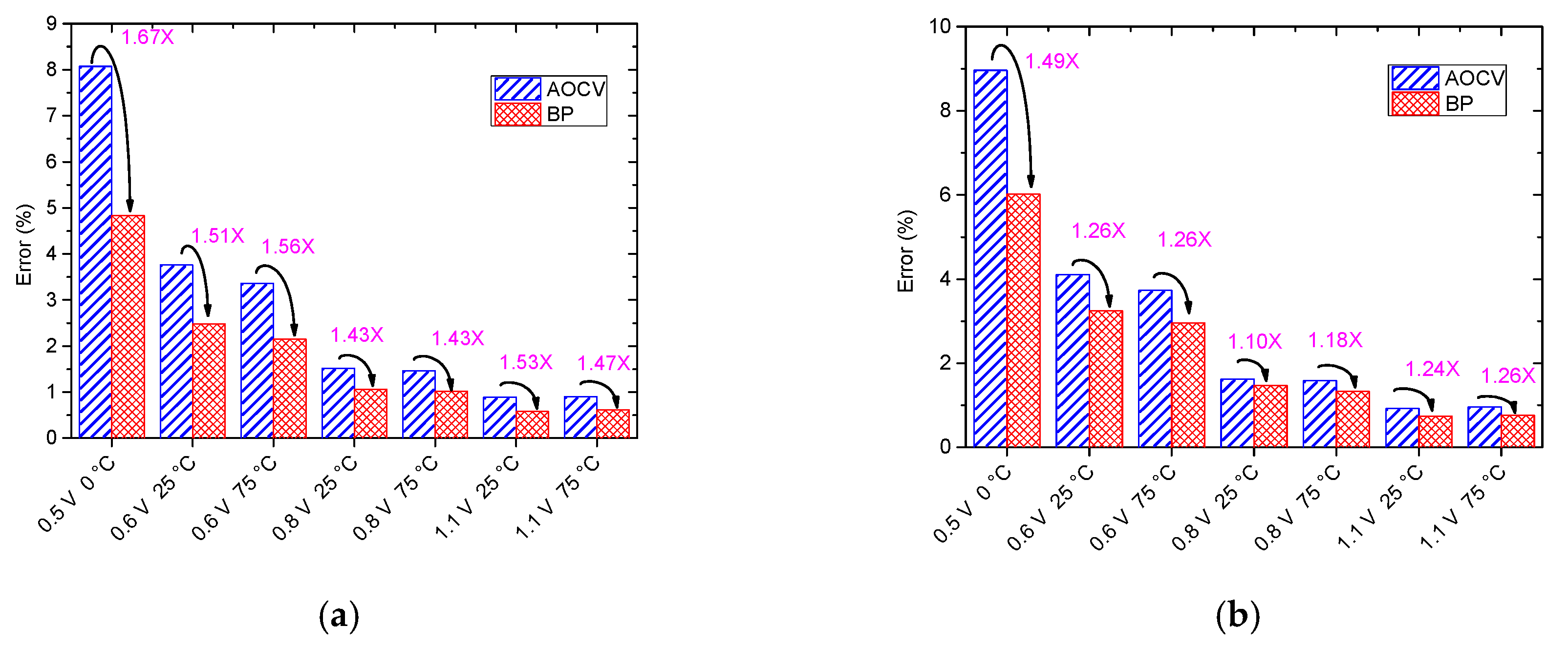
3.2. Path Delay Variation Prediction at Multi-Corner

A single corner demonstrates that the learning-based method performs better than the AOCV method. It should be noted that the AOCV cannot be used in multi-corners to predict unknown corners, so only the result of the BP method is illustrated here. Furthermore, the framework is extended to the multi-corner condition and to predict the corner which is not included in the training set.

Table 3. Training and predicted corners.

	V	0.6	0.7	0.8	0.9	1.0	1.1
T (°C)
0		▲		▲		★	▲
20			★
25		▲		▲			▲
50		★	★		★
75		▲		▲			▲
100			★			★
125		▲		▲			▲

▲: training corner ★: predicted corner.

lists the training corners and predicted corners, where ▲ indicates training corners and ★ expresses predicted corners. Also, the training corners contain train paths and test paths that are characterized in advance, and the predicted corners include new corners and new paths that are different from those in the training set to show the advantage of generalization in the proposed work.

The two kinds of stages (5 and 10) are evaluated, and the mean error of the training corners and the predicted corners are shown in Figure 6. The errors of td_−xσ and td_+xσ increase with decreasing voltage and temperature at the two kinds of stages. Regarding td_−xσ, the error increases from 1.21% to 2.82% for stage 5 and from 0.63% to 1.32% for stage 10. Concerning td_+xσ, the error increases from 1.35% to 4.59% for stage 5 and from 0.6% to 1.82% for stage 10. Besides, the errors in stage 10 are less than stage 5 because, as the number of stages increases, the non-Gaussian phenomenon gradually becomes smaller and the interaction between each stage plays a complementary role, so the error itself will be reduced.

Additionally, the errors are less than those found in previous works, and the detailed comparison is introduced in the following. The proposed prediction method is compared with some different ways proposed in other papers.

Table 4. Comparison with previous works.

	[16]	[25]	This Work
Technology	28 nm	28, 40, 65 nm	40 nm
V	0.5 V	0.3–1.2 V	0.6–1.1 V
T	N/A	70 °C	0–125 °C
Error	5.68% (6.21%)	5.3% (11.4%)	2% (4.59%)
Characterize effort	100SPICE/cell	2000SPICE/cell	1000SPICE/path
Application range	Single T,V	Multiple T,V	Multiple T,V

shows the comparison of our work with that by Alioto et al. [27] and Rithe’s et al. [16]. All three works have good accuracy for the prediction of a given path at a given temperature (T) and voltage (V), especially in near-threshold voltage, of which the distribution is non-Gaussian, and their average prediction errors are all below 6%. The common contributions of the three works are that they all provide a way to predict path delay variation and avoid great timing cost of the MC method.

Compared to the work by Rithe’s et al. [16], the main improvement of our method is that it can handle any temperatures and voltages, as long as the model is established, while in the work by Rithe’s et al. [16], the method is based on the gate timing library and rebuilding all the gate characteristic of a path at a new temperature or voltage. Therefore, the other method is not applicable for multi-corners. Compared to the study by Alioto et al. [27], which regards the delay independent from temperature and voltage at the reference of Fanout of 4 (FO4), it has a good result at multiple temperatures and voltages. Regarding our work, which employed ML, it models the relationships between temperature, voltage and path delay, so it gains a higher accuracy of 2%, on average.

When considering the timing cost for path delay variation prediction, the study by Rithe’s et al. [16] characterizes the statistical delay for every cell in one corner, which will spend about 100 times of SPICE simulations, it can predict any new path delay variation at this corner with the average(max) error of 5.68% (6.21%). When the path delay variation of other corners is needed, the number of SPICE simulations will multiply the number of corners. The FO4 method proposed by Alioto et al. [27] needs 2000 SPICE simulations for each gate characteristic and is appropriate for multiple temperatures and voltages, that is to say, after characterizing every cell, the method can predict any new path at multiple corners within the average(max) error of 5.3% (11.4%). The timing cost of our method mainly stays in the training set build, which needs 1000 SPICE simulations for each path in the training set. Subsequent to the training, the model can provide a new path delay in a new corner with an average(max) of 2% (4.59%), which is the lowest/minimum average error of these methods. Thus, our work provides a promising method for solving the path delay variation problem for single- and multi-corner conditions.

4. Conclusions

Here, the learning-based method was adopted to solve the path delay variation problem under single and multiple corners. First, the characterization effort for the timing library of each cell was eliminated in our work, as well as the computing effort of the non-grid timing by interpolation. Second, the proposed framework predicted the path delay variation at single- and multi-corners. Regarding the single corner, the train/test error was much lower than AOCV, while for multi-corner, the error in stage 10 was much less than that in stage 5, but the predicted errors were within the acceptable range compared with previous works.

References

1. McConaghy, T.; Breen, K.; Dyck, J.; Gupta, A. Variation-Aware Design of Custom Integrated Circuits: A Hands-On Field Guide; Springer Science and Business Media: New York, NY, USA, 2012. [Google Scholar]
2. Abu-Rahma, M.H.; Anis, M. A statistical design-oriented delay variation model accounting for within-die variations. IEEE Trans. Comput. Aided Des. Integr. Circuits Syst. 2008, 27, 1983–1995. [Google Scholar] [CrossRef]
3. Corsonello, P.; Frustaci, F.; Lanuzza, M.; Perri, S. Over/undershooting effects in accurate buffer delay model for sub-threshold domain. IEEE Trans. Circuits Syst. I Regul. Pap. 2014, 61, 1456–1464. [Google Scholar] [CrossRef]
4. Tolbert, J.R.; Mukhopadhyay, S. Accurate buffer modeling with slew propagation in subthreshold circuits. In Proceedings of the International Symposium on Quality Electronic Design, San Jose, CA, USA, 16–18 March 2009; pp. 91–96. [Google Scholar]
5. Takahashi, R.; Takata, H.; Yasufuku, T. Large within-die gate delay variations in sub-threshold logic circuits at low temperature. IEEE Trans. Circuits Syst. II Express Briefs 2012, 12, 918–921. [Google Scholar] [CrossRef]
6. Harris, D.M.; Keller, B.; Karl, J.; Keller, S. A transregional model for near-threshold circuits with application to minimum-energy operation. In Proceedings of the International Conference on Microelectronics, Cairo, Egypt, 19–22 December 2011; pp. 64–67. [Google Scholar]
7. Dreslinski, R.G.; Wieckowski, M.; Blaauw, D. Near-Threshold Computing: Reclaiming Moore’s Law Through Energy Efficient Integrated Circuits. Proc. IEEE 2010, 98, 253–266. [Google Scholar] [CrossRef]
8. Kaul, H.; Anders, M.; Hsu, S.; Agarwal, A. Near-threshold voltage (NTV) design: Opportunities and challenges. In Proceedings of the 49th Annual Design Automation Conference, San Francisco, CA, USA, 3–7 June 2012; pp. 1153–1158. [Google Scholar]
9. Markovic, D.; Wang, C.C.; Alarcon, L.P. Ultralow-Power Design in Near-Threshold Region. Proc. IEEE 2010, 98, 237–252. [Google Scholar] [CrossRef]
10. Datta, B.; Burleson, W. Temperature effects on energy optimization in sub-threshold circuit design. In Proceedings of the International Symposium on Quality Electronic Design, San Jose, CA, USA, 16–18 March 2009; pp. 680–685. [Google Scholar]
11. Kuhn, K.J.; Giles, M.D.; Becher, D.; Kolar, P.; Kornfeld, A.; Kotlyar, R.; Mudanai, S. Process technology variation. IEEE Trans. Electron Devices 2011, 58, 2197–2208. [Google Scholar] [CrossRef]
12. Shoniker, M.; Oleynikov, O.; Cockburn, B.F.; Han, J.; Rana, M.; Pedrycz, W. Automatic Selection of Process Corner Simulations for Faster Design Verification. IEEE Trans. Comput. Aided Des. Integr. Circuits Syst. 2017, 37, 1312–1316. [Google Scholar] [CrossRef]
13. De Jonghe, D.; Maricau, E.; Gielen, G.; McConaghy, T.; Tasić, B.; Stratigopoulos, H. Advances in variation-aware modeling, verification, and testing of analog ICs. In Proceedings of the Conference on Design, Automation and Test in Europe, Dresden, Germany, 12–16 March 2012; pp. 1615–1620. [Google Scholar]
14. Alioto, M. Ultra-low power VLSI circuit design demystified and explained: A tutorial. IEEE Trans. Circuits Syst. I Regul. Pap. 2012, 59, 3–29. [Google Scholar] [CrossRef]
15. Keller, S.; Harris, D.M.; Martin, A.J. A compact transregional model for digital CMOS circuits operating near threshold. IEEE Trans. Very Large Scale Integr. Syst. 2014, 22, 2041–2053. [Google Scholar] [CrossRef]
16. Rithe, R.; Gu, J.; Wang, A.; Datla, S.; Gammie, G.; Buss, D.; Chandrakasan, A. Non-linear operating point statistical analysis for local variations in logic timing at low voltage. In Proceedings of the Conference on Design, Automation and Test in Europe, Dresden, Germany, 8–12 March 2010; pp. 965–968. [Google Scholar]
17. Zhang, Y.; Calhoun, B.H. Fast, accurate variation-aware path timing computation for sub-threshold circuits. In Proceedings of the Fifteenth International Symposium on Quality Electronic Design, Santa Clara, CA, USA, 3–5 March 2014; pp. 243–248. [Google Scholar]
18. Shiomi, J.; Ishihara, T.; Onodera, H. Statistical Timing Modeling Based on a Lognormal Distribution Model for Near-Threshold Circuit Optimization. IEICE Trans. Fundam. Electron. Commun. Comput. Sci. 2015, 98, 1455–1466. [Google Scholar] [CrossRef] [Green Version]
19. Guo, J.; Zhu, J.; Wang, M.; Nie, J.; Liu, X.; Ge, W.; Yang, J. Analytical inverter chain’s delay and its variation model for sub-threshold circuits. IEICE Electron. Express 2017, 14, 20170390. [Google Scholar] [CrossRef] [Green Version]
20. Frustaci, F.; Corsonello, P.; Perri, S. Analytical delay model considering variability effects in subthreshold domain. IEEE Trans. Circuits Syst. II Express Briefs 2012, 59, 168–172. [Google Scholar] [CrossRef]
21. Zhang, G.; Li, B.; Liu, J.; Shi, Y.; Schlichtmann, U. Design-phase buffer allocation for post-silicon clock binning by iterative learning. IEEE Trans. Comput. Aided Des. Integr. Circuits Syst. 2017, 37, 392–405. [Google Scholar] [CrossRef] [Green Version]
22. Zhang, G.; Li, B.; Liu, J.; Schlichtmann, U. Sampling-based buffer insertion for post-silicon yield improvement under process variability. In Proceedings of the Design Automation & Test in Europe Conference & Exhibition (DATE), Dresden, Germany, 14–18 March 2016; pp. 1457–1460. [Google Scholar]
23. Orshansky, M.; Nassif, S.; Boning, D. Design for Manufacturability and Statistical Design: A Constructive Approach; Springer Science & Business Media: New York, NY, USA, 2007. [Google Scholar]
24. Khandelwal, V.; Srivastava, A. A quadratic modeling-based framework for accurate statistical timing analysis considering correlations. IEEE Trans. Very Large Scale Integr. Syst. 2007, 15, 206–215. [Google Scholar] [CrossRef] [Green Version]
25. Li, B.; Chen, N.; Xu, Y.; Schlichtmann, U. On timing model extraction and hierarchical statistical timing analysis. IEEE Trans. Comput. Aided Des. Integr. Circuits Syst. 2013, 32, 367–380. [Google Scholar] [CrossRef] [Green Version]
26. Hong, J.; Huang, K.; Pong, P.; Pan, J.D.; Kang, J.; Wu, K.C. An LLC-OCV methodology for statistic timing analysis. In Proceedings of the IEEE International Symposium on VLSI Design, Automation and Test (VLSI-DAT), Hsinchu, Taiwan, 25–27 April 2007; pp. 1–4. [Google Scholar]
27. Alioto, M.; Scotti, G.; Trifiletti, A. A novel framework to estimate the path delay variability on the back of an envelope via the fan-out-of-4 metric. IEEE Trans. Circuits Syst. I Regul. Pap. 2017, 64, 2073–2085. [Google Scholar] [CrossRef]
28. Cohen, E.; Malka, D.; Shemer, A.; Shahmoon, A.; Zalevsky, Z.; London, M. Neural networks within multi-core optic fibers. Sci. Rep. 2016, 6, 29080. [Google Scholar] [CrossRef] [Green Version]
29. Malka, D.; Vegerhof, A.; Cohen, E.; Rayhshtat, M.; Libenson, A.; Aviv Shalev, M.; Zalevsky, Z. Improved Diagnostic Process of Multiple Sclerosis Using Automated Detection and Selection Process in Magnetic Resonance Imaging. Appl. Sci. 2017, 7, 831. [Google Scholar] [CrossRef] [Green Version]
30. Malka, D.; Berke, B.A.; Tischler, Y.; Zalevsky, Z. Improving Raman spectra of pure silicon using super-resolved method. J. Opt. 2019, 21, 075801. [Google Scholar] [CrossRef]
31. Das, B.P.; Amrutur, B.; Jamadagni, H.S.; Arvind, N.V.; Visvanathan, V. Voltage and temperature-aware SSTA using neural network delay model. IEEE Trans. Semicond. Manuf. 2011, 24, 533–544. [Google Scholar] [CrossRef]
32. Kahng, A.B.; Luo, M.; Nath, S. SI for free: Machine learning of interconnect coupling delay and transition effects. In Proceedings of the ACM/IEEE International Workshop on System Level Interconnect Prediction (SLIP), San Francisco, CA, USA, 6 June 2015; pp. 1–8. [Google Scholar]
33. Han, S.S.; Kahng, A.B.; Nath, S.; Vydyanathan, A.S. A deep learning methodology to proliferate golden signoff timing. In Proceedings of the conference on Design, Automation & Test in Europe, Dresden, Germany, 24–28 March 2014; p. 260. [Google Scholar]
34. Yi, J.; Wang, Q.; Zhao, D.; Wen, J.T. BP neural network prediction-based variable-period sampling approach for networked control systems. Appl. Math. Comput. 2007, 185, 976–988. [Google Scholar] [CrossRef]
35. Li, Y.; Fu, Y.; Li, H.; Zhang, S.W. The improved training algorithm of back propagation neural network with self-adaptive learning rate. IEEE Int. Conf. Comput. Intell. Nat. Comput. 2009, 1, 73–76. [Google Scholar]
Figure 1. The flowchart of the prediction framework for path delay variation based on ML algorithm.
Electronics 09 00157 g001
Figure 2. The architecture of the BP model.
Electronics 09 00157 g002
Figure 3. The trade-off of sample number and accuracy at different conditions. (a) 0.6 V 25 °C, (b) 0.6 V 75 °C, (c) 0.8 V 25 °C, (d) 0.8 V 75 °C.
Electronics 09 00157 g003
Figure 4. Path variation delay training error at td−xσ at a single corner. (a) train error; (b) test error.
Electronics 09 00157 g004
Figure 5. Path variation delay predicted error at td+xσ at a single corner. (a) train error; (b)test error.
Electronics 09 00157 g005
Figure 6. Path variation delay mean error prediction of stage 5 and 10 at multi-corner conditions. (a) t d x σ ; (b) t d + x σ .
Electronics 09 00157 g006