Article

Deep Learning-Based Stacked Denoising and Autoencoder for ECG Heartbeat Classification

by
Siti Nurmaini
*,
Annisa Darmawahyuni
,
Akhmad Noviar Sakti Mukti
,
Muhammad Naufal Rachmatullah
,
Firdaus Firdaus
and
Bambang Tutuko
Intelligent System Research Group, Universitas Sriwijaya, Palembang 30139, Indonesia
*
Author to whom correspondence should be addressed.
Electronics 2020, 9(1), 135; https://doi.org/10.3390/electronics9010135
Submission received: 16 December 2019 / Revised: 8 January 2020 / Accepted: 8 January 2020 / Published: 10 January 2020
(This article belongs to the Special Issue Sensing and Signal Processing in Smart Healthcare)

Abstract

:
The electrocardiogram (ECG) is a widely used, noninvasive test for analyzing arrhythmia. However, the ECG signal is prone to contamination by different kinds of noise. Such noise may cause deformation on the ECG heartbeat waveform, leading to cardiologists’ mislabeling or misinterpreting heartbeats due to varying types of artifacts and interference. To address this problem, some previous studies propose a computerized technique based on machine learning (ML) to distinguish between normal and abnormal heartbeats. Unfortunately, ML works on a handcrafted, feature-based approach and lacks feature representation. To overcome such drawbacks, deep learning (DL) is proposed in the pre-training and fine-tuning phases to produce an automated feature representation for multi-class classification of arrhythmia conditions. In the pre-training phase, stacked denoising autoencoders (DAEs) and autoencoders (AEs) are used for feature learning; in the fine-tuning phase, deep neural networks (DNNs) are implemented as a classifier. To the best of our knowledge, this research is the first to implement stacked autoencoders by using DAEs and AEs for feature learning in DL. Physionet’s well-known MIT-BIH Arrhythmia Database, as well as the MIT-BIH Noise Stress Test Database (NSTDB). Only four records are used from the NSTDB dataset: 118 24 dB, 118 −6 dB, 119 24 dB, and 119 −6 dB, with two levels of signal-to-noise ratio (SNRs) at 24 dB and −6 dB. In the validation process, six models are compared to select the best DL model. For all fine-tuned hyperparameters, the best model of ECG heartbeat classification achieves an accuracy, sensitivity, specificity, precision, and F1-score of 99.34%, 93.83%, 99.57%, 89.81%, and 91.44%, respectively. As the results demonstrate, the proposed DL model can extract high-level features not only from the training data but also from unseen data. Such a model has good application prospects in clinical practice.

1. Introduction

The electrocardiogram (ECG) is a valuable technique for making decisions regarding cardiac heart diseases (CHDs) [1]. However, the ECG signal acquisition involves high-gain instrumentation amplifiers that are easily contaminated by different sources of noise, with characteristic frequency spectrums depending on the source [2]. ECG contaminants can be classified into different categories, including [2,3,4]; (i) power line interference at 60 or 50 Hz, depending on the power supply frequency; (ii) electrode contact noise of about 1 Hz, caused by improper contact between the body and electrodes; (iii) motion artifacts that produce long distortions at 100–500 ms, caused by patient’s movements, affecting the electrode–skin impedance; (iv) muscle contractions, producing noise up to 10% of regular peak-to-peak ECG amplitude and frequency up to 10 kHz around 50 ms; and (v) baseline wander caused by respiratory activity at 0–0.5 Hz. All of these kinds of noise can interfere with the original ECG signal, which may cause deformations on the ECG waveforms and produce an abnormal signal.
To keep as much of the ECG signal as possible, the noise must be removed from the original signal to provide an accurate diagnosis. Unfortunately, the denoising process is a challenging task due to the overlap of all the noise signals at both low and high frequencies [4]. To prevent noise interference, several approaches have been proposed to denoise ECG signals based on adaptive filtering [5,6,7], wavelet methods [8,9], and empirical mode decomposition [10,11]. However, all these proposed techniques require analytical calculation and high computation; also, because cut-off processing can lose clinically essential components of the ECG signal, these techniques run the risk of misdiagnosis [12]. Currently, one machine learning (ML) technique, named denoising autoencoders (DAEs), can be applied to reconstruct clean data from its noisy version. DAEs can extract robust features by adding noise to the input data [13]. Previous results indicate that DAEs outperform conventional denoising techniques [14,15,16]. Recently, DAEs have been used in various fields, such as image denoising [17], human activity recognition [18], and feature representation [19].
To produce the proper interpretation of CHDs, the ECG signal must be classified after the denoising process. However, DAEs are unable to automatically produce the extracted feature [15,16]. Feature extraction is an important phase in the classification process for obtaining robust performance. If feature representation is bad, it will cause the classifier to produce a low performance. Such a limitation in DAEs leaves room for further improvement upon the existing ECG denoising method through combination with other methods for feature extraction. Some techniques, including principal component analysis (PCA) or linear discriminant analysis (LDA) algorithms, have been proposed [20,21]. However, these cannot extract the feature directly from the network structure and they usually require a trial-and-error process, which is time-consuming [20,21]. Currently, by using autoencoders (AEs), extracting features of the raw input data can work automatically. This leads to an improvement in the prediction model performances, while, at the same time, reducing the complexity of the feature design task. Hence, a combination of two models of DAEs and AEs is a challenging task in ECG signal processing applications.
The classification phase based on ECG signal processing studies can be divided into two types of learning: supervised and unsupervised [22,23,24,25,26,27]. Such two types of learning provide good performance in ECG beats [26,27,28], or rhythm classification [27,28,29]. Among them, Yu et al. [26] proposed higher-order statistics of sub-band components for heartbeat classification with noisy ECG. Their proposed classifier is a feedforward backpropagation neural network (FBNN). The feature selection algorithm is based on the correlation coefficient with five levels of the discrete wavelet transform (DWT). However, for exceptional evaluation, DWT becomes computationally intensive. Besides its discretization, DWT is less efficient and less natural, and it takes time and energy to learn which wavelets will serve each specific purpose. Li et al. [27] focused on the five-level ECG signal quality classification algorithm, adding three types of real ECG noise at different signal-to-noise ratio (SNR) levels. A support vector machine (SVM) classifier with a Gaussian radial basis function kernel was employed to classify the ECG signal quality. However, ECG signal classification with traditional ML based on supervised shallow architecture is limited by feature extraction and classification because it uses a handcrafted, feature-based approach. Also, for larger amounts of ECG data and variance, the shallow architecture can be employed for this purpose. On the other hand, the deep learning (DL) technique extracts features directly from data [24,25]. In our previous work [30], the DL technique successfully worked to generate feature representations from raw data. This process is carried out by conducting an unsupervised training approach to process feature learning and followed by a classification process. DL has superiority in automated feature learning, while ML is only limited to feature engineering.
Artificial neural networks (ANNs) are a well-known technique in ML. ANNs increase the depth of structure by adding multiple hidden layers, named deep neural networks (DNNs). Some of these layers can be adjusted to better predict the final outcome. More layers enable DNNs to fit complex functions with fewer parameters and improve accuracy [27]. Compared with shallow neural networks, DNNs with multiple nonlinear hidden layers can discover more complex relationships between input layers and output layers. High-level layers can learn features from lower layers to obtain higher-order and more abstract expressions of inputs [28]. However, DNNs cannot learn features from noisy data. The combination of DNNs and autoencoders (AEs) can learn efficient data coding in an unsupervised manner. However, the AEs do not perform well when the data samples are very noisy [28]. Therefore, DAEs were invented to enable AEs to learn features from noisy data by adding noise to the input data [28].
To the best of our knowledge, no research has implemented the DL technique using stacked DAEs and AEs to accomplish feature learning for the noisy signal of ECG heartbeat classification. This paper proposes a combination DAEs–AEs–DNNs processing method to calculate appropriate features from ECG raw data to address automated classification. This technique consists of beat segmentation, noise cancelation with DAEs, feature extraction with AEs, and heartbeat classification with DNNs. The validation and evaluation of classifiers are based on the performance metrics of accuracy, sensitivity, specificity, precision, and F1-score. The rest of this paper is organized as follows. In Section 2, we explain the materials and the proposed method. In Section 3, we conduct an experiment on a public dataset and compare the proposed method with existing research. Finally, we conclude the paper and discuss future work in Section 4.

2. Research Method

2.1. Autoencoder

Autoencoders (AEs) are a neural network trained to try to map the input to its output in an unsupervised manner. AEs have a hidden layer h that describes the coding used to represent the input [29]. AEs consist of two parts—the encoder ( h = f ( a ) ) and the decoder ( r = g ( h ) ) network. f and g are called the encoder and decoder mappings, respectively. The number of hidden units is smaller than the input or output layers, which achieve encoding of the data in a lower-dimensional space and extract the most discriminative features. Given the training samples D (dimensional vectors) a = { a 1 , a 2 , , a m } , the encoder forms the x  input vector into d (dimensional vectors), a hidden representation h = { h 1 , h 2 , , h m } . This study implements the rectified linear unit (ReLU) as an activation function in the first hidden encoding layer. In addition, the activation function σ , h = σ ( W ( 1 ) x + b ( 1 ) ) , in the output, where W ( 1 )  is a d × D (dimensional weight matrix), and b ( 1 ) is a d (dimensional bias vector). Then, vector h is transformed back into the reconstruction vector r = { r 1 , r 2 , . , r m } by the decoder z = σ ( W ( 2 ) h + b ( 2 ) ) , where r is a D (dimensional vector), W ( 2 ) is a D × d (dimensional weight matrix), and b ( 2 ) is a D (dimensional bias vector). The AEs’ training aims to optimize the parameter set θ = { W ( 1 ) , b ( 2 ) , W ( 2 ) , b ( 2 ) } for reducing the error of reconstruction. The mean squared error (MSE) is used as a loss function in standard AEs [26,30]:
ι M S E ( θ ) = 1 m i = 1 m L M S E ( x i , z i ) = 1 m i = 1 m ( 1 2 | | z i x i | | 2 )
AEs are usually trained using only a clean ECG signal dataset. For the further task of treating noisy ECG data, denoising AEs (DAEs) are introduced. In the case of a single-hidden-layer neural AE trained with noisy ECG data as input and a clean signal as an output, it includes one nonlinear encoding and decoding stage, as follows:
y = f ( x ˜ i ) = σ ( W 2 x ˜ i + b )
and
z = g ( y ) = σ ( W 2 y + c )
where x ˜ is a corrupted version of x, b and c represent vectors of biases of input and output layers, respectively, and x is the desired output. Usually, a tied weight matrix (i.e., W 1 = W 2 T = W ) is used as one type of regularization. This paper uses a noisy signal to train the DAEs before the automated feature extraction with AEs. DAEs are a stochastic extension of classic AEs. DAEs try to reconstruct a clean input from its corrupted version. The initial input x is corrupted to x ˜ by a stochastic mapping x ˜ q ( x ˜ | x ) . Subsequently, DAEs use the corrupted x ˜ as the input data and then map to the corresponding hidden representation y and ultimately to its reconstruction z . After the reconstruction signal is obtained from DAEs, the signal-to-noise ratio (SNRs) value must be calculated so that the signal quality can be measured [30], as follows:
S N R = 10 log 10 [ n x d 2 ( n ) n ( x d ( n ) x ( n ) ) 2 ]
where x d and x are the reconstructed and the original signal, respectively.
DAEs have shown good results in extracting noisy robust features in ECG signals and other applications [14].

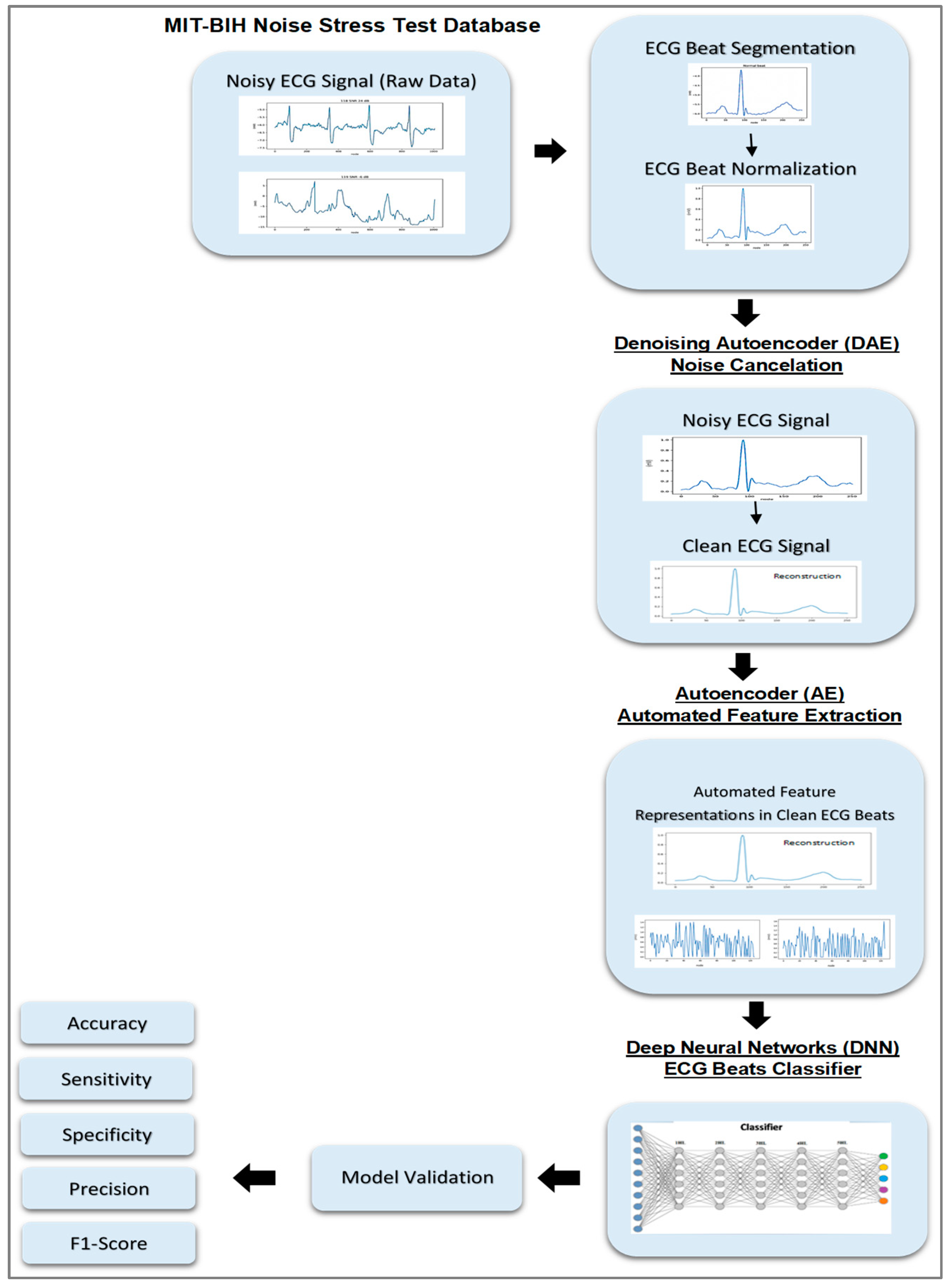
2.2. Proposed Deep Learning Structure

The basis of DL is a bio-inspired algorithm from the earliest neural network. Fundamentally, DL formalizes how a biological neuron works, in which the brain can process information by billions of these interlinked neurons [30]. DL has provided new advanced approaches to the training of DNNs architectures with many hidden layers, outperforming its ML counterpart. The features extracted in DL by using data-driven methods can be more accurate. An autoencoder is a neural network designed specifically for this purpose. In our previous work [30], deep AEs were shown to be implemented in ECG signal processing before the classification task, extracting high-level features not only from the training data but also from unseen data. The Softmax function is used as an activation function, and it can be treated as the probability of each label for the output layer of the classifier. Here, let N be the number of units of the output layer, let x be the input, and let x i be the output of unit i . Then, the output p ( i ) of unit i is defined by the following equation,
p ( i ) = e x i j = 1 N e x j
Cross entropy is used as the loss function of the classifier L f , as follows:
L f ( θ ) = 1 n i = 1 n j = 1 m y i j log ( p i j )
where n is the sample size, m is the number of classes, p i j  is the output of the classifier of class j of the i t h  sample, and y i j  is the annotated label of class j of the i t h  sample.
In our study, the proposed DL structure consists of noise cancelation with DAEs, automated feature extraction with AEs, and DNNs as a classifier, as presented in Figure 1. DAEs structure is divided into three layers, namely the input, encoding, and output layer. There are two models of DAEs structured for validation—Model 1, which has an input, encoding, and output layer which each have 252 nodes, respectively, while in Model 2 the input and output layers have 252 nodes, respectively, and the encoding layer has 126 nodes. For all models, the activation function in the encoding layer is the rectified linear unit (ReLU) and in the output layer is sigmoid. The compilation of the DAEs model requires two arguments, namely the optimizer and loss function. The optimization method used in the DAE construction is adaptive moment estimation (Adam), with the mean squared error as the loss function. As the proposed DAEs structure, SNR −6 dB is used for the input as the noisiest ECG and SNR 24 dB for the desired signal as the best ECG quality in the dataset used in this study. After doing some experiments and completing the training phase, a good accuracy with a total of 400 epochs and a batch size of 64 is obtained. Then, the DAEs model can already be used to reconstruct the signal with SNR −6 dB, and the results of the reconstructed signal will approach an SNR of 24 dB.
After all noisy signals have been removed by the DAEs, the next process is to extract the features of the signal. Automated feature extraction using the AEs [30] is the final step before the ECG heartbeat can be classified using DNNs. The ECG signal that has been reconstructed by the DAEs is carried out in a training process with 200 epochs and a batch size of 32 for the AE architecture. After completing the AEs’ training phase, the reconstruction signal is used for prediction in the encoder, from the input layer to the encoding layer. After the signal is predicted in the encoder, a feature of the reconstructed signal is obtained. This reconstructed signal is used as the classifier input of the DNNs. Like the DAEs architecture, ReLU and Sigmoid were implemented in the encoding layer and output layer, respectively. The encoding layer of the AEs is used as an input for the DNNs classifier, which has five hidden layers and represents five classes of ECG heartbeat. In the input layer, there are 32, 63, and 126 nodes, which refer to the length of each feature signal. Then, in the output layer, there are 5 nodes, which represent the number of classified ECG heartbeat classes. Each of the hidden layers has 100 nodes. The DNNs architecture was conducted by ReLU in all hidden layers and by Softmax in the output layer. The loss function of categorical cross-entropy and Adam optimizer are also implemented in the proposed DNNs architecture. This DNNs architecture was trained to as many as 200 epochs with a batch size of 48.

2.3. Experimental Result

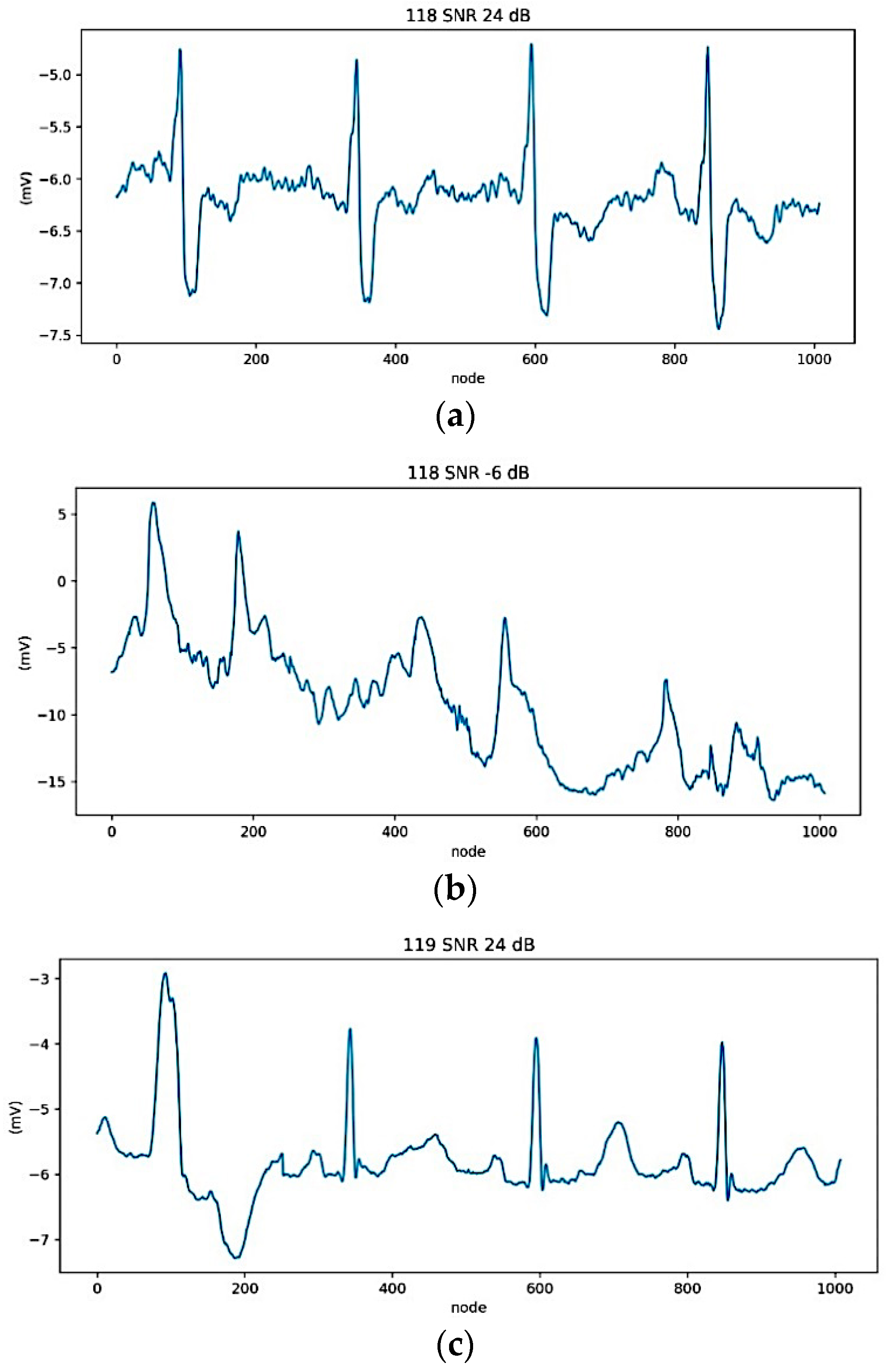
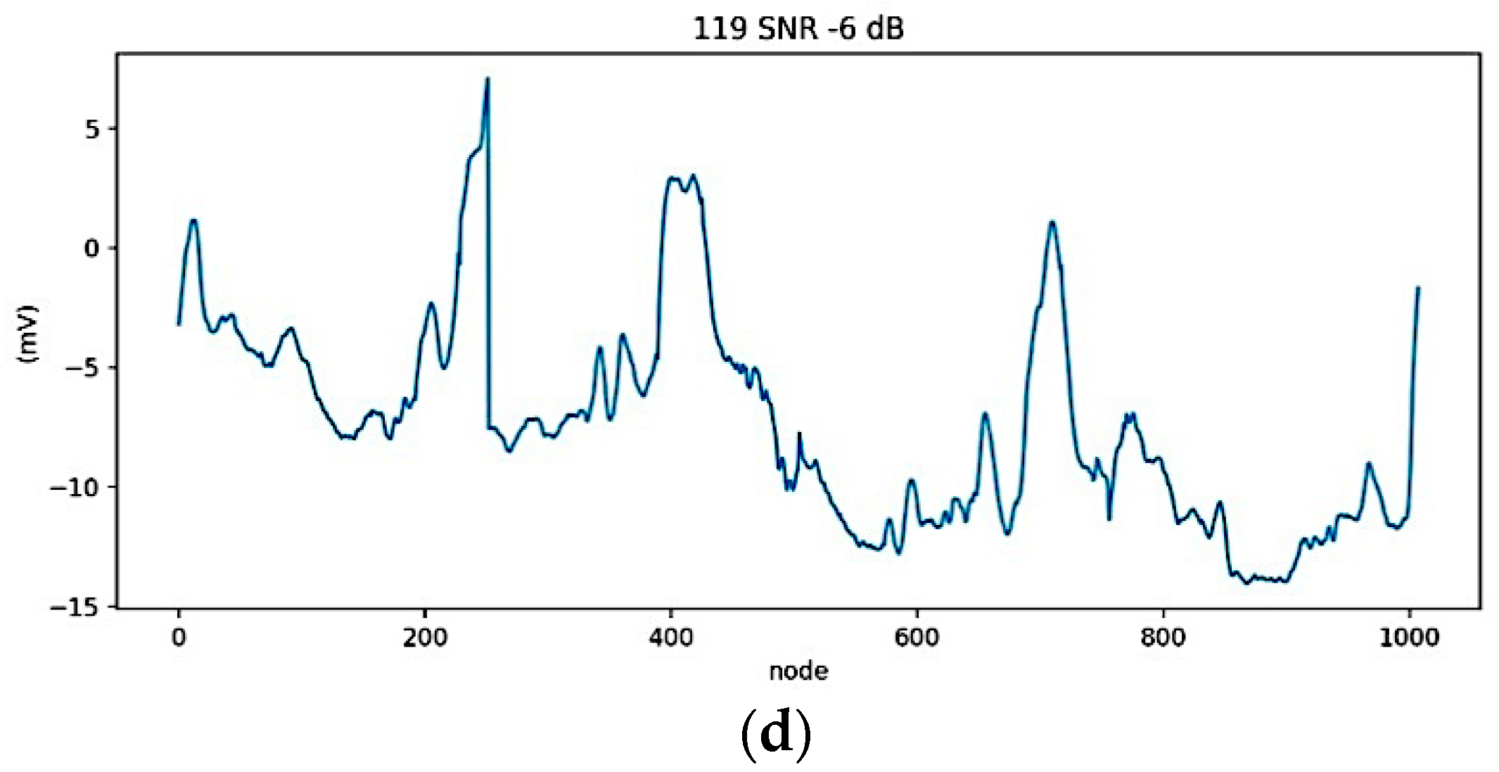
2.3.1. Data Preparation

The raw data were taken from ECG signals from the MIT-BIH Arrhythmia Database (MITDB), and the added noise signals were obtained from the MIT-BIH Noise Stress Test Database (NSTDB). The available source can be accessed at https://physionet.org/content/nstdb/1.0.0/. This database includes 12 half-hour ECG recordings and 3 half-hour recordings of noise typical in ambulatory ECG recordings. Only two recordings (the 118 and 119 records) from the MITDB are used for the NSTDB. From the MITDB’s two clean recordings, the NSTDB records consisted of six levels of SNR, from the best to the worst ECG signal quality: 24 dB, 18 dB, 12 dB, 6 dB, 0 dB, and −6 dB. The NSTDB consists of 12 half-hour ECG recordings and 3 half-hour ECG noise recordings. Only two levels of SNRs were used in this study—the SNRs of 24 dB and −6 dB, the best and the worst ECG signal quality, respectively. The two levels consisted of four records; 118 24 dB, 118 −6 dB, 119 24 dB, and 119 −6dB were used in this study. SNRs of –6dB and 24 dB were processed by the DAEs. The ECG raw data are represented in Figure 2.

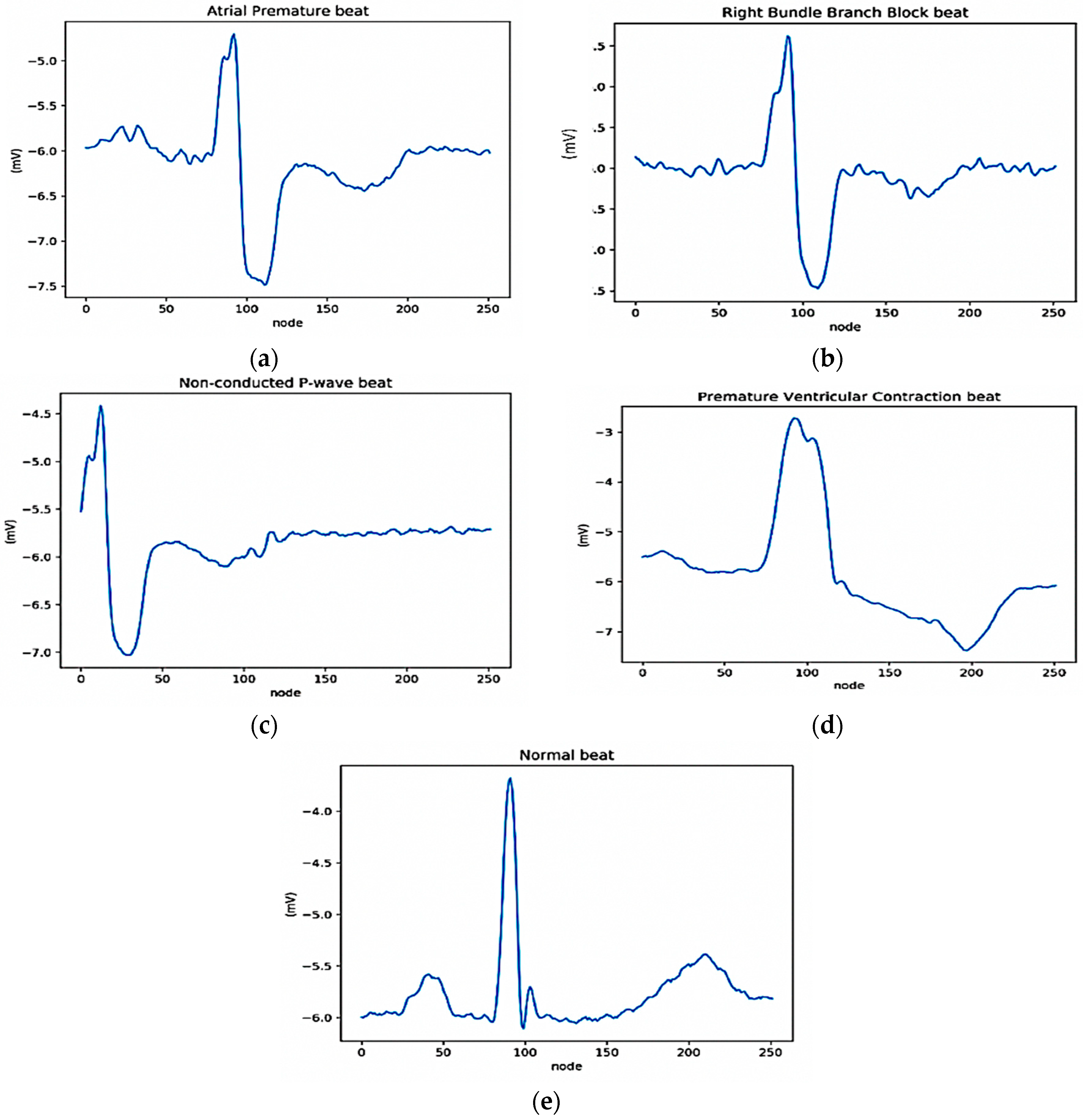
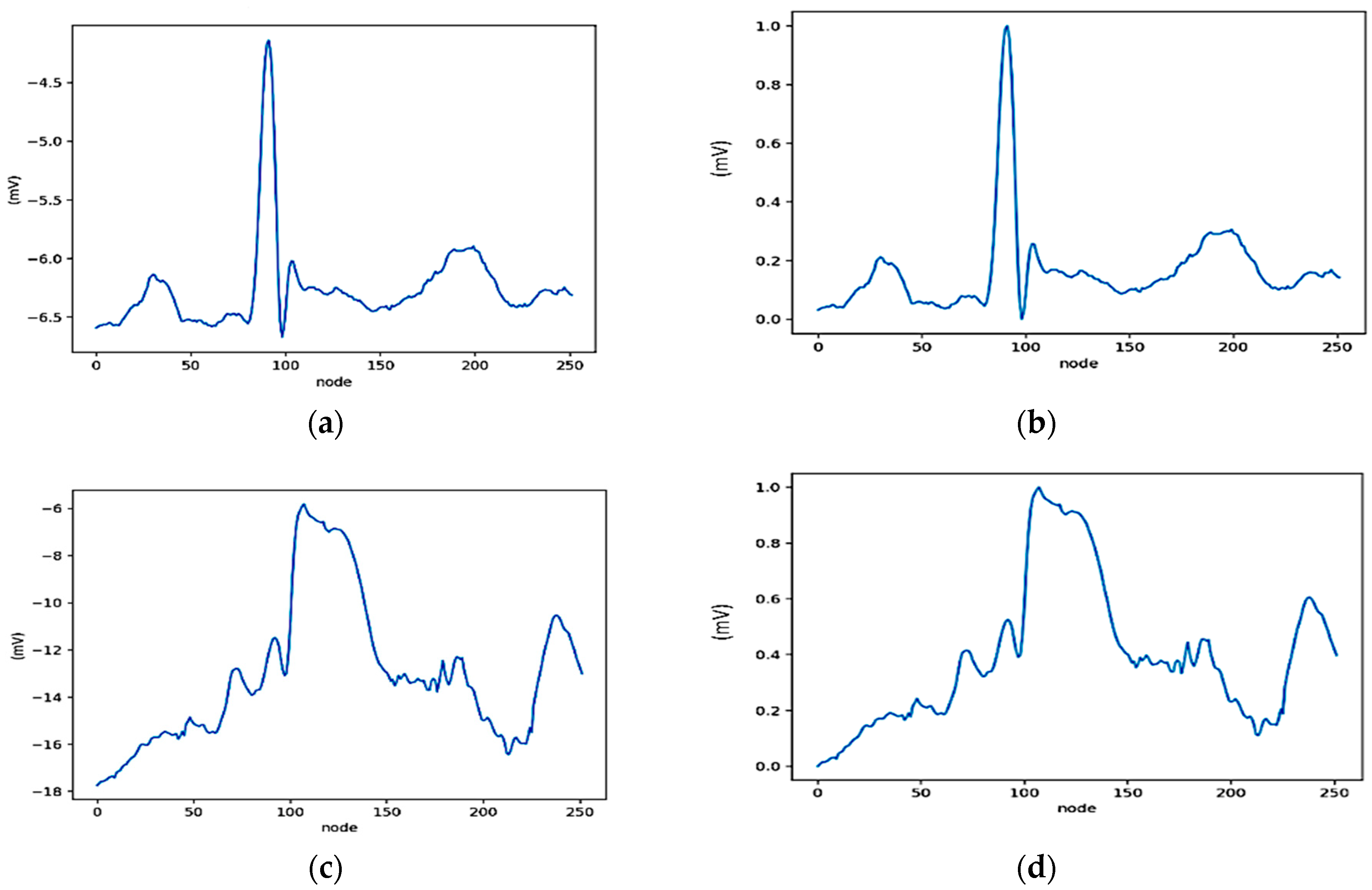
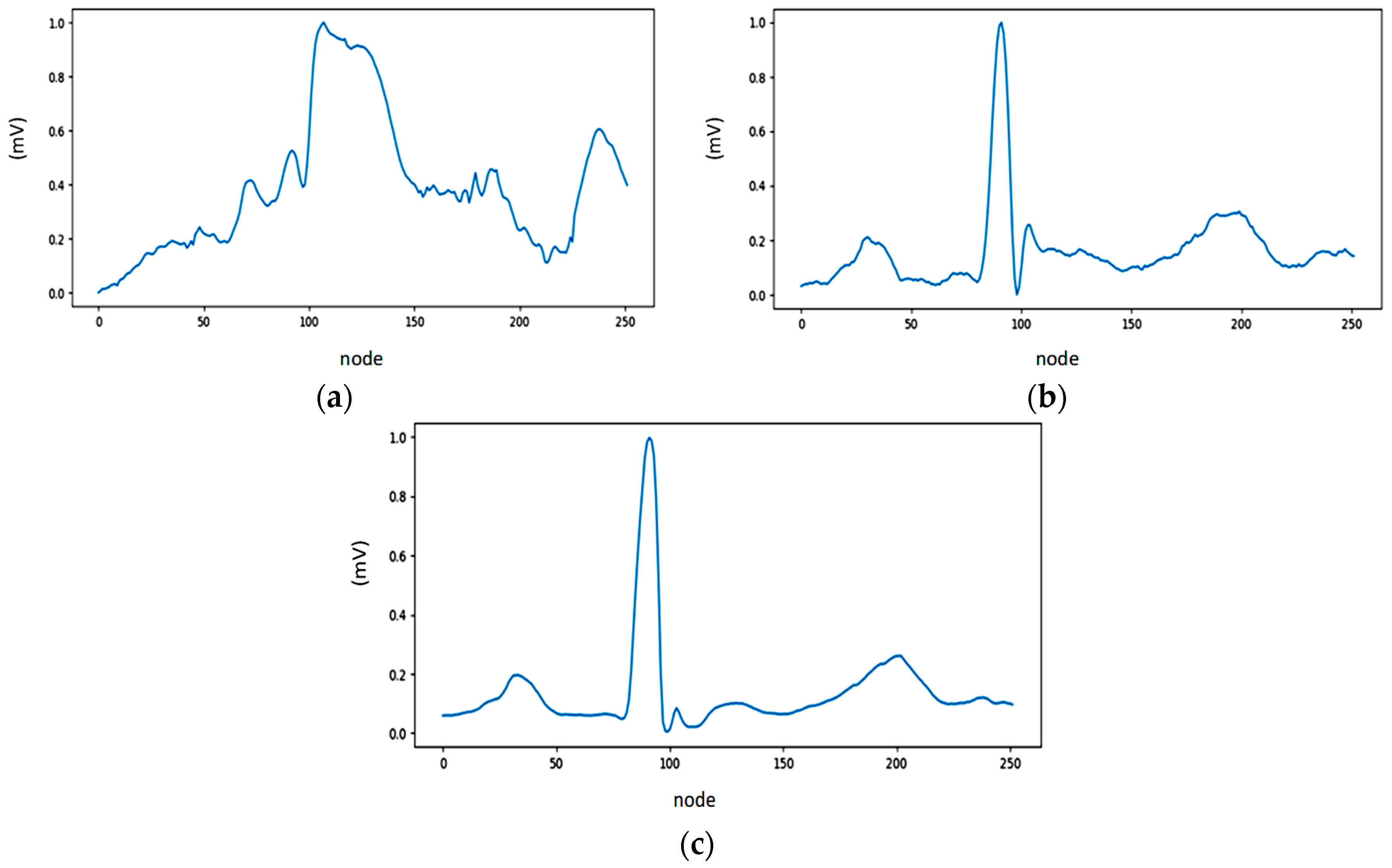
2.3.2. ECG Segmentation and Normalization

In our previous work [30], ECG signal segmentation was used to find the R-peak position. After the R-peak position was detected, sampling was performed at approximately 0.7-s segments for a single beat. The section was divided into two intervals: t1 of 0.25 s before the R-peak position and t2 of 0.45 s after the R-peak position. The ECG records of 118 24 dB, 118 −6 dB, 119 24 dB, and 119 −6 dB were segmented into the beat (see Figure 3).
The record of 118 contained four types of heartbeat: Atrial Premature (A), Right Bundle Branch Block (R), Non-conducted P-wave (P), and Premature Ventricular Contraction (V). The record of 119 contains two types of heartbeat: Normal (N) and Premature Ventricular Contraction (V). The total beats of each record were 2287 and 1987, respectively. The number and representation of each beat are represented in Table 1, and the sample of a heartbeat after segmentation in Figure 4.
After the segmentation of each beat, the ECG signal was normalized into 0 and 1 using the normalized bound. Normalized bound changed the value of the lower limit ( l b ) and upper limit ( u b ) on the amplitude of a signal to the desired range without changing the pattern or shape of the signal itself. In this study, the data was acquired in the pre-process with the lower limit (0) and upper limit (1), respectively. The mathematical function of the normalization with normalized bound is as follows:
f ( x ) = x c o e f ( x m i d c o e f ) + m i d
where
c o e f = ( u b l b x max x min )
x m i d is the midpoint of the input signal:
x m i d = x max x max x min 2
x max is the peak point of the input signal, x min is the lower point of the input signal, and m i d is the midpoint of the specified limit:
m i d = u b u b l b 2
The sample result of normalized ECG beats can be seen in Figure 5, in which the range of amplitude (mV) of signal is 0 and 1.

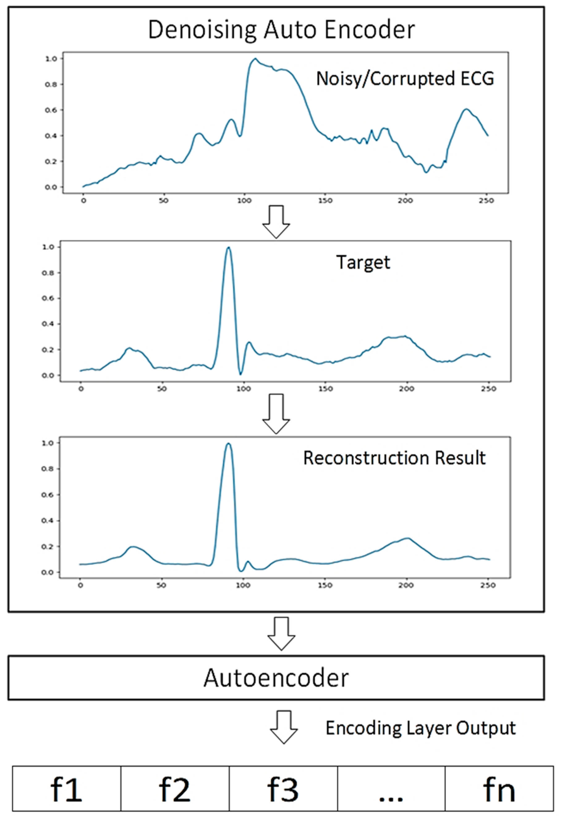
2.3.3. Pre-Training and Fine-Tuning

The DL structure was formed by combining the pre-training DAEs’ and AEs’ encoding layers and the fine-tuning of the DNN algorithm with the fully connected layer. For the first model, ECG noise removal was based on the DAEs structure with 252 nodes in each of its encoding layers. Then, the second model used 126 nodes in the encoding layer. For the first model produced by the DAEs, the loss average was 0.0029, and the SNR reconstruction was 23.1527 dB. The DAEs’ second model produced a loss of 0.0037 and a SNR reconstruction of 20.6129 dB. Both models had the desired SNRs of 25.8182 dB. Comparing the two models, the SNR reconstruction for the first model was 23.1527 dB and 20.6129 dB for the second. It can be concluded that the first model had a higher SNR than the second model. Higher SNRs were achieved, producing a better result for the reconstructed signal. Therefore, for the AEs’ automated feature extraction, the DAEs’ first model with 252 nodes was used, and the result of the ECG construction can be seen in Figure 6.
After the DAEs model was trained, a reconstruction result (clean ECG signal) was produced. A clean ECG signal was used as an input into the AEs model to extract features. The feature was learned through the encoder and decoder steps. After the AEs model was trained, the encoder part was used as the feature output, and all features (f1, f2, f3, … fn) were used as an input into the DNNs model to classify the ECG heartbeat. All steps of feature learning are presented in Figure 7. In the third and fourth models there were five layers, in which there are 63 nodes in the encoding layer. For the fifth and sixth models, we propose seven layers, in which there are 32 nodes in the encoding layer. Based on our previous work [30], for all six models in this study, we propose ReLU and Softmax activation functions with Adam optimization (0.0001 as the learning rate). Adam optimization allows for the use of adaptive learning levels for each variable. The total epoch of each model is 200, with a batch size of 48.
To select a good classifier model, the DAEs, AEs, and DNNs change in some structures in the validation phase. Only DL with high performance is selected as the best DL model. This paper presents a total of six models for ECG heartbeat classification validation (see Table 2). The weights of the classifier are extracted from the pre-trained DAEs–AEs model, and the fully connected layer is added as an output layer with Softmax as an activation function and categorical cross-entropy as a loss function.
The classification performances were measured by using the following five metrics in the literature: accuracy, sensitivity, specificity, precision and F1-score [22,30]. While accuracy can be used for evaluating the overall performance as benchmarking, the other metrics can measure the performance of a specific class of validation model. The five metrics that measured for model validation can be expressed as follows:
A c c u r a c y = i = 1 l T P i + i = 1 l T N i i = 1 l T P i + i = 1 l T N i + i = 1 l F P i + i = 1 l F N i
S e n s i t i v i t y = i = 1 l T P i i = 1 l T P i + i = 1 l F N i
S p e c i f i c i t y = i = 1 l T N i i = 1 l T N i + i = 1 l F P i
P r e c i s i o n = i = 1 l T P i i = 1 l T P i + i = 1 l F N i
F 1 S c o r e = i = 1 l T P i i = 1 l T P i + i = 1 l F N i
where I is the number of beat classes; T P i (true positives) is the number of class i t h that are correctly classified; T N i (true negative) is the number of non-class i t h that are correctly classified; F P i (false positive) is the number of non-class i t h that are incorrectly predicted as class i t h types, and F N i (false negative) is the number of class i t h that are incorrectly predicted as non-class i t h .

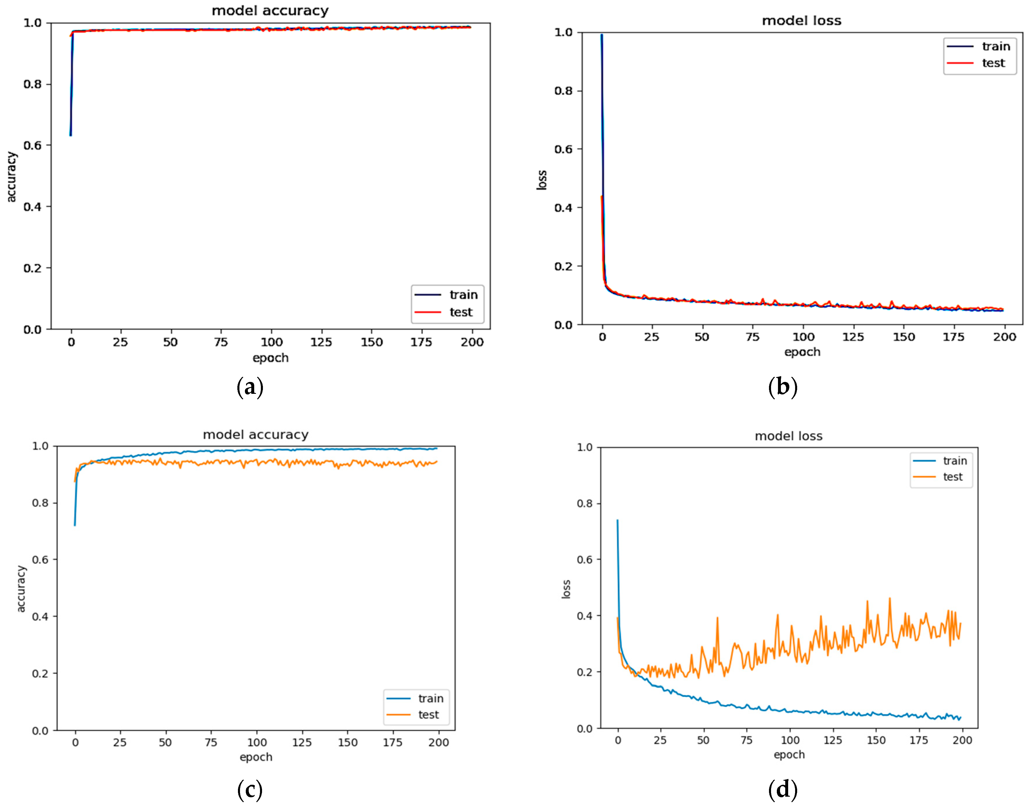
3. Results and Analysis

In this study, the training process used 90% of the data, and the remaining data was used for the testing process. The testing set was used to make decisions on hyperparameter values and model selection in Table 2. The next procedure was the classification stage with DNNs after the feature had been extracted in the AEs. Firstly, in the input layer, different nodes were compared: 32, 63, and 126. Then, the fine-tuned nodes were used to obtain the best architecture in the input layer. As seen in Table 2, the first model of DNNs, with 126 nodes, was chosen because it outperformed the other nodes in the result. The architecture of the first DNNs model consisted of one input layer, five hidden layers (each with 100 nodes), and the output layers which represented five classes of ECG beat (i.e., A, R, P, V, and N). In the output layers, we applied the Softmax function. To evaluate our proposed DNNs model, five performance metrics were used: accuracy, sensitivity, specificity, precision, and F1-score. The comparison result based on these metrics of the six DL models in Table 2 is shown in Table 3 and Table 4, for the training and testing sets, respectively. As displayed in Table 3, Model 1 yields the highest accuracy, specificity, precision, and F1-score in the training phase. For the testing results in Table 4, Model 1 also yields the highest results in all performance metrics. Therefore, Model 1 is our proposed DL architecture for ECG noise removal and AEs feature extraction to the DNNs classification task. Unfortunately, poor performances were shown in Models 5 and 6. This is because Models 5 and 6 use the DAEs’ second model that produced a loss of 0.0037 and SNR reconstruction of 20.6129 dB. This reconstruction is not close to the target signal of 24 dB, meaning that the ECG is still noisy. This will affect the classifier’s performance results at the end. The sensitivity, precision, and F1-score achieved only 56.97% to 59.19%. The sensitivity of Model 5 in training is inversely proportional to the testing set. In training, the sensitivity is 98.90%; however, in testing, it only achieves 56.97%. As seen in Table 2 and Table 4, the number of AE encoding layers in Models 5 and 6 yields the worst result in the testing phase of the classifier.
As for classification, to analyze the prediction of the DL model in each class during the training and testing phase, the confusion matrix was applied. Table 5 and Table 6 present the predicted ECG heartbeat class only for the first model as the proposed architecture. For the A-class (atrial premature beat), compared to the R class (right bundle branch block), there are 11 misclassified ECG heartbeats in the training phase and only two misclassified beats in the testing phase. From the result of the confusion matrix, the A-class is the worst result of all the classes. Beats were misclassified as R beats in both the training and testing phases. This may have occurred because of the larger amount of data for R beats compared to A beats. This may have occurred due to such a large amount of comparison data for the A and R beats. Later, the morphology between these two beats is similar.
In this study, we compared the classification process of two types of feature-learning condition: with and without AEs. However, by excluding the AEs structure, the comparison is conducted only for the best models of DNNs structure. Such conditions help investigate what affects the DNNs’ classifier performance without feature extraction. With the same DL architecture with DAEs, the result of the testing phase is presented in Table 7. Table 7 shows a significant gap between the DAEs–AEs–DNNs model and the DAEs–DNNs model. The DAEs–AEs–DNNs model outperformed the DAEs–DNNs model for all five ECG beat classes, with average scores of 99.34%, 93.83%, 99.575%, 89.81%, and 91.44% in accuracy, sensitivity, specificity, precision, and F1-score, respectively. Without AEs, the result of all the performance metrics decreases significantly, including a concerningly poor performance score of 78.67% in precision. DAEs are trained in a similar yet different way. When performing the self-supervised training, the input ECG signal is corrupted by adding noise. The DAEs, whose task is to recover the original input, are trained locally to denoise corrupted versions of their inputs. However, sometimes the input and expected output of ECG are not identical, which affects the DNNs classifier. Therefore, the DAEs are stacked with AEs as a solution to provide a good representation for a better-performing classifier. Intuitively, if a representation allows for a proper reconstruction of its input, it means that it has retained much of the information that was present in that input.
To verify the proposed DL model, the accuracy and the loss curve are shown in Figure 8a,b, respectively. In Figure 8a, the accuracy of the training set starts above 60% in the first epoch. Later, in the testing set, the accuracy of the model achieves a satisfactory accuracy of about 99.34%. Figure 8b shows decreasing error until 0.6%, along with increasing epochs in the training and testing set. Both curves produce suitable shapes, as the DAEs and AEs’ reconstruction results show effective noise cancelation before processing with the DNNs. However, after 60 rounds of training, the DL cannot predict accurately when AEs are not included in the structure (see Figure 8c,d). This shows that while DAEs perform the denoising process to reconstruct the clean data, they fail to reconstruct the representation feature for the classifier. Without AEs, the input to DNNs is the DAE’s encoding. Therefore, the output classifier reaches a 40% loss in the testing process and produces overfitting due to the ECG beats’ signal being incorrectly predicted by the DNNs (see Figure 8c). As seen in Figure 8d, the training error is much lower than the testing error, thus producing a high variance.
The performance of the proposed DL structure was compared to three previous studies in the literature [26,27,31], due to limited previous research classifying heartbeats with noisy data using ML including SVM, FBNNs, and CNNs (see Table 8). The results found that, with an accuracy level of 99.34%, our proposed DL structure outperformed the SVM, FBNN, and CNN classifiers of ECG noise removal and feature representation algorithms (see Table 8). The proposed DL structure yields higher accuracy than FBNNs, SVM, and CNNs, which yield 97.50%, 80.26%, and 95.70% accuracy, respectively. We can clearly observe that the proposed DL model with stacked DAEs–AEs successfully reconstructs the heartbeat ECG signal from the noisy signal and is effective for arrythmia diagnosis. In our previous research [30], the DL model with DWT for noise cancelation was proposed with the MITDB dataset without noise stress. This study took the best DL model from [30] and added data from the NSTDB, producing a higher than 99% accuracy for two conditions of the ECG signal. This means the proposed DL model may be generalizable in arrhythmia diagnosis.

4. Conclusions

ECG heartbeat classification is still an interesting issue in medical applications. The classification process is not a simple task because the ECG may get corrupted by noise during acquisition due to different types of artifacts and signal interference. The noise of the ECG can affect cardiologists’ misinterpretation of arrhythmia cases. To overcome such problems, a deep learning (DL) approach is presented in this study. We exploit DAEs for noise cancellation, AEs for feature learning and DNNs for classification. In our DL structure, the DAEs and AEs structure is staked to produce good feature representation. To the best of our knowledge, this research is the first to stack autoencoders by using DAEs and AEs for feature learning. The encoding layer of the DAEs was implemented in the signal reconstructed with the AEs. Afterward, six DL models were compared to select the best classifier architecture. All DL models were validated by using the MIT-BIH Noise Stress Test Database. The result shows that the proposed DL model demonstrates superior automated feature learning as compared to a shallow ML model. ML requires human interference and expertise in determining robust features, making it time-consuming in the labelling and data processing steps. Moreover, the proposed DL structure is able to extract high-level features not only from the training data but also from unseen data. For all fine-tuned hyperparameters, the best model of ECG heartbeat classifier is the first model (Model 1) with one hidden layer in DAEs, one hidden layer in AEs and five hidden layers in DNNs. Such a DL model produces accuracy, sensitivity, specificity, precision, and F1-score of 99.34%, 93.83%, 99.57%, 89.81%, and 91.44%, respectively. Moreover, the proposed DL model with stacked DAEs and AEs, outperforms another DL structure without AEs. However, this study put greater focus on feature learning with denoising ECG signals. Therefore, the practicality and generalizability of multiple measurements of the ECG recording must be improved in the future to ensure the proposed method is suitable for clinical diagnosis with the widely used 12-lead ECG. With the collection of more abnormal ECG recordings, we hope to produce a good classifier for diagnosing more cardiac diseases with our proposed DL models.

Author Contributions

S.N. Conceptualization, resources, supervision, and writing—review & editing; A.D. Formal analysis, software, and writing—original draft; A.N.S.M. Software; M.N.R. Software and writing—review & editing; F.F. Writing—review & editing; B.T. writing—review & editing. All authors have read and agreed to the published version of the manuscript.

Funding

This work was supported by Basic Research Grants (096/SP2H/LT/DRPM/2019) from the Ministry of Research, Technology, and Higher Education and Unggulan Profesi Grants from Universitas Sriwijaya Indonesia.

Acknowledgments

The authors are very thankful to Wahyu Caesarendra, Universiti Brunei Darussalam, for his valuable comments, discussion, and suggestions for improving the paper.

Conflicts of Interest

The authors declare no conflict of interest.

References

  1. Guaragnella, C.; Rizzi, M.; Giorgio, A. Marginal Component Analysis of ECG Signals for Beat-to-Beat Detection of Ventricular Late Potentials. Electronics 2019, 8, 1000. [Google Scholar] [CrossRef] [Green Version]
  2. Castillo, E.; Morales, D.P.; Garcia, A.; Martinez-Marti, F.; Parrilla, L.; Palma, A.J. Noise suppression in ECG signals through efficient one-step wavelet processing techniques. J. Appl. Math. 2013, 2013. [Google Scholar] [CrossRef]
  3. Antczak, K. Deep Recurrent Neural Networks for ECG Signal Denoising. arXiv 2018, arXiv:1807.11551. [Google Scholar]
  4. Wang, D.; Si, Y.; Yang, W.; Zhang, G.; Li, J. A Novel Electrocardiogram Biometric Identification Method Based on Temporal-Frequency Autoencoding. Electronics 2019, 8, 667. [Google Scholar] [CrossRef] [Green Version]
  5. Meireles, A.J.M. ECG Denoising Based on Adaptive Signal Processing Technique. Master’s Thesis, Instituto Politécnico do Porto, Instituto Superior de Engenharia do Porto, Porto, Portugal, 2011. [Google Scholar]
  6. Joshi, V.; Verma, A.R.; Singh, Y. De-noising of ECG signal using Adaptive Filter based on MPSO. Procedia Comput. Sci. 2015, 57, 395–402. [Google Scholar] [CrossRef] [Green Version]
  7. Sharma, I.; Mehra, R.; Singh, M. Adaptive filter design for ECG noise reduction using LMS algorithm. In Proceedings of the 2015 4th International Conference on Reliability, Infocom Technologies and Optimization (ICRITO) (Trends and Future Directions), Noida, India, 2–4 September 2015; pp. 1–6. [Google Scholar]
  8. Aqil, M.; Jbari, A.; Bourouhou, A. ECG Signal Denoising by Discrete Wavelet Transform. Int. J. Online Eng. 2017, 13. [Google Scholar] [CrossRef]
  9. Srivastava, M.; Anderson, C.L.; Freed, J.H. A new wavelet denoising method for selecting decomposition levels and noise thresholds. IEEE Access 2016, 4, 3862–3877. [Google Scholar] [CrossRef]
  10. Kong, Q.; Song, Q.; Hai, Y.; Gong, R.; Liu, J.; Shao, X. Denoising signals for photoacoustic imaging in frequency domain based on empirical mode decomposition. Optik (Stuttg) 2018, 160, 402–414. [Google Scholar] [CrossRef]
  11. Nguyen, P.; Kim, J.-M. Adaptive ECG denoising using genetic algorithm-based thresholding and ensemble empirical mode decomposition. Inf. Sci. (N. Y.) 2016, 373, 499–511. [Google Scholar] [CrossRef]
  12. Yoon, D.; Lim, H.S.; Jung, K.; Kim, T.Y.; Lee, S. Deep Learning-Based Electrocardiogram Signal Noise Detection and Screening Model. Healthc. Inform. Res. 2019, 25, 201–211. [Google Scholar] [CrossRef]
  13. Vincent, P.; Larochelle, H.; Bengio, Y.; Manzagol, P.-A. Extracting and composing robust features with denoising autoencoders. In Proceedings of the 25th International Conference on Machine Learning, Helsinki, Finland, 5–9 July 2008; pp. 1096–1103. [Google Scholar]
  14. Chiang, H.-T.; Hsieh, Y.-Y.; Fu, S.-W.; Hung, K.-H.; Tsao, Y.; Chien, S.-Y. Noise Reduction in ECG Signals Using Fully Convolutional Denoising Autoencoders. IEEE Access 2019, 7, 60806–60813. [Google Scholar] [CrossRef]
  15. Xiong, P.; Wang, H.; Liu, M.; Liu, X. Denoising autoencoder for eletrocardiogram signal enhancement. J. Med. Imaging Heal. Inform. 2015, 5, 1804–1810. [Google Scholar] [CrossRef]
  16. Xiong, P.; Wang, H.; Liu, M.; Lin, F.; Hou, Z.; Liu, X. A stacked contractive denoising auto-encoder for ECG signal denoising. Physiol. Meas. 2016, 37, 2214. [Google Scholar] [CrossRef] [PubMed]
  17. Xing, C.; Ma, L.; Yang, X. Stacked denoise autoencoder based feature extraction and classification for hyperspectral images. J. Sens. 2016, 2016. [Google Scholar] [CrossRef] [Green Version]
  18. Yang, J.; Nguyen, M.N.; San, P.P.; Li, X.L.; Krishnaswamy, S. Deep convolutional neural networks on multichannel time series for human activity recognition. In Proceedings of the Twenty-Fourth International Joint Conference on Artificial Intelligence, Buenos Aires, Argentina, 25–31 July 2015. [Google Scholar]
  19. Budiman, A.; Fanany, M.I.; Basaruddin, C. Stacked denoising autoencoder for feature representation learning in pose-based action recognition. In Proceedings of the 2014 IEEE 3rd Global Conference on Consumer Electronics (GCCE), Tokyo, Japan, 7–10 October 2014; pp. 684–688. [Google Scholar]
  20. Nurmaini, S.; Partan, R.U.; Rachmatullah, M.N. Deep Neural Networks Classifiers on The Electrocardiogram Signal for Intelligent Interpretation System. Sriwij. Int. Conf. Med. Sci. 2018. [Google Scholar] [CrossRef]
  21. Martis, R.J.; Acharya, U.R.; Min, L.C. ECG beat classification using PCA, LDA, ICA and discrete wavelet transform. Biomed. Signal Process. Control 2013, 8, 437–448. [Google Scholar] [CrossRef]
  22. Qin, Q.; Li, J.; Zhang, L.; Yue, Y.; Liu, C. Combining low-dimensional wavelet features and support vector machine for arrhythmia beat classification. Sci. Rep. 2017, 7, 6067. [Google Scholar] [CrossRef] [PubMed] [Green Version]
  23. Hermans, B.J.M.; Stoks, J.; Bennis, F.C.; Vink, A.S.; Garde, A.; Wilde, A.A.M.; Pison, L.; Postema, P.G.; Delhaas, T. Support vector machine-based assessment of the T-wave morphology improves long QT syndrome diagnosis. EP Eur. 2018, 20, iii113–iii119. [Google Scholar] [CrossRef]
  24. Faziludeen, S.; Sankaran, P. ECG beat classification using evidential K-nearest neighbours. Procedia Comput. Sci. 2016, 89, 499–505. [Google Scholar] [CrossRef] [Green Version]
  25. Hejazi, M.; Al-Haddad, S.A.R.; Singh, Y.P.; Hashim, S.J.; Aziz, A.F.A. Multiclass support vector machines for classification of ECG data with missing values. Appl. Artif. Intell. 2015, 29, 660–674. [Google Scholar] [CrossRef]
  26. Yu, S.-N.; Chen, Y.-H. Noise-tolerant electrocardiogram beat classification based on higher order statistics of subband components. Artif. Intell. Med. 2009, 46, 165–178. [Google Scholar] [CrossRef] [PubMed]
  27. Li, Q.; Rajagopalan, C.; Clifford, G.D. A machine learning approach to multi-level ECG signal quality classification. Comput. Methods Programs Biomed. 2014, 117, 435–447. [Google Scholar] [CrossRef] [PubMed]
  28. Übeyli, E.D. ECG beats classification using multiclass support vector machines with error correcting output codes. Digit. Signal Process. 2007, 17, 675–684. [Google Scholar] [CrossRef]
  29. Sugimoto, K.; Kon, Y.; Lee, S.; Okada, Y. Detection and localization of myocardial infarction based on a convolutional autoencoder. Knowl. Based Syst. 2019, 178, 123–131. [Google Scholar] [CrossRef]
  30. Nurmaini, S.; Partan, R.U.; Caesarendra, W.; Dewi, T.; Rahmatullah, M.N.; Darmawahyuni, A.; Bhayyu, V.; Firdaus, F. An Automated ECG Beat Classification System Using Deep Neural Networks with an Unsupervised Feature Extraction Technique. Appl. Sci. 2019, 9, 2921. [Google Scholar] [CrossRef] [Green Version]
  31. Ochiai, K.; Takahashi, S.; Fukazawa, Y. Arrhythmia Detection from 2-lead ECG using Convolutional Denoising Autoencoders. In Proceedings of the KDD’18 Deep Learning Day, London, UK, 19–23 August 2018. [Google Scholar]
Figure 1. The proposed deep learning (DL) structures.
Electronics 09 00135 g001
Figure 2. Electrocardiogram (ECG) raw data with noise. (a) Record 118 (24 dB), (b) Record 118 (−6 dB), (c) Record 119 (24 dB), (d) Record 119 (−6 dB).
Electronics 09 00135 g002aElectronics 09 00135 g002b
Figure 3. The ECG segmentation process.
Electronics 09 00135 g003
Figure 4. Heartbeat segmentation result. (a) Beat 959 label A (record 118), (b) Beat 72 label R (record 118), (c) Beat 2018 label P (record 118), (d) Beat 2323 label V (record 119), (e) Beat 2320 label N (record 119).
Electronics 09 00135 g004
Figure 5. The sample of normalized beats in record 119. (a) ECG signal 24 dB before normalization, (b) ECG signal 24 dB after normalization, (c) ECG signal −6 dB before normalization, (d) ECG signal −6 dB after normalization.
Electronics 09 00135 g005
Figure 6. The sample of denoising autoencoders (DAEs)–autoencoders (AEs) process for ECG signal. (a) Noisy ECG Signal, (b) Target, (c) Reconstruction.
Electronics 09 00135 g006
Figure 7. The sample of the stacked DAEs–AEs process for ECG signal.
Electronics 09 00135 g007
Figure 8. DL performance based on accuracy and loss curves. (a) Accuracy curve (DAEs–AEs–DNNs), (b) Loss curve (DAEs–AEs–DNNs), (c) Accuracy curve (DAEs–DNNs), (d) Loss curve (DAEs–DNNs).
Electronics 09 00135 g008
Table 1. Heartbeat distribution after the ECG segmentation.
BeatsRecord of 118Record of 119Total
NNone15431543
V16444460
R2165None2165
A96None96
P10None10
Total228719874274
Table 2. Model validation of ECG heartbeat classification.
ModelDAEsAEsDNNs
1(252-252-252)
(ReLU-Sigmoid)
Autoencoder
(252-126-252)
(ReLU-Sigmoid)
(126-100-100-100-100-100-5)
(ReLU-ReLU-ReLU-ReLU-ReLU-Softmax)
2(252-252-252)
(ReLU-Sigmoid)
Deep Autoencoder
(252-126-63-126-252)
(ReLU-ReLU-ReLU-Sigmoid)
(63-100-100-100-100-100-5)
(ReLU-ReLU-ReLU-ReLU-ReLU-Softmax)
3(252-252-252)
(ReLU-Sigmoid)
Deep Autoencoder
(252-126-63-32-63-126-252)
(ReLU-ReLU-ReLU-ReLU-ReLU-Sigmoid)
(32-100-100-100-100-100-5)
(ReLU-ReLU-ReLU-ReLU-ReLU-Softmax)
4(252-126-252)
(ReLU-Sigmoid)
Autoencoder
(252-126-252)
(ReLU-Sigmoid)
(126-100-100-100-100-100-5)
(ReLU-ReLU-ReLU-ReLU-ReLU-Softmax)
5(252-126-252)
(ReLU-Sigmoid)
Deep Autoencoder
(252-126-63-126-252)
(ReLU-ReLU-ReLU-Sigmoid)
(63-100-100-100-100-100-5)
(ReLU-ReLU-ReLU-ReLU-ReLU-Softmax)
6(252-126-252)
(ReLU-Sigmoid)
Deep Autoencoder
(252-126-63-32-63-126-252)
(ReLU-ReLU-ReLU-ReLU-ReLU-Sigmoid)
(32-100-100-100-100-100-5)
(ReLU-ReLU-ReLU-ReLU-ReLU-Softmax)
Table 3. The performance evaluation of DL models in the training phase.
TrainingValidation Model (%)
Metrics123456
Accuracy99.4999.3999.2699.1499.0398.93
Sensitivity95.9496.8393.0094.5998.9098.84
Specificity99.6899.6699.5299.5599.4999.40
Precision91.2387.6287.6677.8078.0673.51
F1-Score93.1390.3589.5881.1079.0876.18
Table 4. The performance evaluation of DL models in the testing phase.
TestingModel Validation (%)
Metrics123456
Accuracy99.3499.0699.0698.9798.2298.41
Sensitivity93.8379.5493.5679.0756.9757.49
Specificity99.5799.3399.3599.4398.7598.94
Precision89.8187.6389.4279.9059.1959.37
F1-Score91.4481.8091.1179.4858.0458.40
Table 5. Confusion matrix in the training phase.
ClassARPVN
A4937000
R111937000
P00900
V0004131
N00001389
Table 6. Confusion matrix in the testing phase.
ClassARPVN
A55000
R2215000
P00100
V000460
N0000154
Table 7. The comparison results of DAEs–AEs–DNNs and DAEs–DNNs.
ArchitecturePerformance Metrics (%)
AccuracySensitivitySpecificityPrecisionF1-Score
DAEs–DNNs
(without AEs)
96.9585.2397.6778.6780.52
DAEs–AEs–DNNs
(proposed model)
99.3493.8399.5789.8191.44
Table 8. The benchmark of the proposed model with another DL structure.
AuthorsDatasetNoise CancelationFeature ExtractionClassifierCaseAccuracy (%)
Yu et al. [26]MITDBDWTCorrelation coefficientFBNNsBeats classification97.50
Li et al. [27]MITDBFilterVarianceSVMECG signal quality80.26
Ochiai et al. [31]MITDBDAEsCNNsCNNs 1D/2DBeats classification95.70
Nurmaini et al. [30]MITDBDWTAEsDNNsBeats classification99.73
ProposedMITDB with NSTDBDAEsAEsDNNsBeats classification99.34

