A Semidefinite Relaxation Method for Elliptical Location

Abstract

Wireless location is a supporting technology in many application scenarios of wireless communication systems. Recently, an increasing number of studies have been conducted on range-based elliptical location in a variety of backgrounds. Specifically, the design and implementation of position estimators are of great significance. The difficulties arising from implementing a maximum likelihood estimator for elliptical location come from the nonconvexity of the negative log-likelihood functions. The need for computational efficiency further enhances the difficulties. Traditional algorithms suffer from the problems of high computational cost and low initialization justifiability. On the other hand, existing closed-form solutions are sensitive to the measurement noise levels. We recognize that the root of these drawbacks lies in an oversimplified linear approximation of the nonconvex model, and accordingly design a maximum likelihood estimator through semidefinite relaxation for elliptical location. We relax the elliptical location problems to semidefinite programs, which can be solved efficiently with interior-point methods. Additionally, we theoretically analyze the complexity of the proposed algorithm. Finally, we design and carry out a series of simulation experiments, showing that the proposed algorithm outperforms several widely used closed-form solutions at a wide range of noise levels. Extensive results under extreme noise conditions verify the deployability of the algorithm.

1. Introduction

During the deployment of powerful location-based applications such as enhanced 911 services, asset management, and workflow automation, wireless location is a classical problem and has attracted intensive research recently [1,2,3,4,5,6]. Technically, wireless location can be based on a variety of different kinds of measurements, such as range [7], angle [8], energy [9], visible light [10,11], or fingerprinting [12,13,14]. The common range-based measurements include time of arrivals (TOAs) [15,16] and time difference of arrivals (TDOAs) [17,18]. TDOAs (or TOAs) are combined to produce intersecting hyperbolic (or circular) lines from which the target location is determined. In addition to these two measurement schemes, there is a less well-known range-based approach called elliptical location [19,20,21,22,23,24,25,26,27]. In particular, in a wireless location system with multiple transmitters and multiple receivers, the sum of each pair of transmitter-target range and target-receiver range defines an ellipse, and the target resides on the intersection of all these ellipses.

Depending on whether the transmitters and receivers are synchronized in time, we have the synchronous elliptical location (SEL) [20,23,24] and the asynchronous elliptical location (AEL) [19,21,22,25,26,27]. For more information on the differences between SEL and AEL, we refer the reader to [28] and references therein. In particular, AEL has been employed in multistatic sonar [21,22,26,27] and indoor location [25,29]. The asynchronous elliptical range measurement between a transmitter and a receiver is the arrival time difference between the indirect signal reflected/relayed from the target and the direct signal from the transmitter. The range measurements can be obtained by auto-correlating the signals at a receiver, or by estimating the indirect and direct arrival times with respect to a local receiver clock and subtracting them. After obtaining the range measurements, AEL and SEL can be formalized as a parameter estimation problem. However, as we will see in Section 2, this estimation problem is very challenging.

In designing the target position estimators, there is no essential differences between SEL and AEL. In view of this fact, we do not distinguish synchronous signal models from asynchronous ones when reviewing the estimation algorithms in the literature. Reference [23] employed the classic spherical-interpolation (SI) [30] and spherical-intersection (SX) [31] methods. The localization accuracy is not optimum in [23]. Reference [26] used Wiener filtering to combine the multiple cross fixes of the ellipses. Reference [25] reformulated the elliptical location problem as a constrained least squares problem and solved it with the method of Lagrange multipliers, resulting in an estimator whose performance is close to the Cramér–Rao bound (CRB). It seems that [23,25,26] only considered the location systems with one transmitter/receiver. Such an assumption is helpful for simplifying the solution of the problem, but the algorithms designed under this assumption are not easy to extend to the scenarios with multiple receivers and multiple transmitters.

More generally, for the elliptical location systems with multiple transmitters and multiple receivers, many researchers [20,22,32,33] made significant exploration. Reference [33] handled the problem through linearizing the measurement equations and searching iteratively. The solution of [33] could be sensitive to the initialization and have the problem of divergence. On the other hand, Reference [32] borrowed the idea of two-stage weighted least squares (WLS) [34] to attack the problem of SEL, which can be easily generalized to AEL. Unfortunately, the solution in [32] is sensitive to the measurement noise levels. More recently, Reference [21] transformed [22]’s four-stage WLS method to a two-stage WLS (TS-WLS) one, and Reference [20] approximated the maximum likelihood estimator (MLE) by the solution of a constrained WLS (CWLS) optimization problem. However, currently proposed methods usually either cannot obtain good performance at high noise levels or have local convergence problems, which may degrade their performance.

As an emerging technology, with its successful application in the field of signal processing [35,36,37,38,39], convex optimization is widely used in the design and implementation of wireless location estimators. Among various convex optimization techniques, semidefinite programming (SDP) can be solved globally in polynomial time while providing an impressive modeling capability [40,41]. On the other hand, owing to the nonconvex nature of the maximum likelihood estimation problems in wireless locations, it is difficult to obtain their globally optimal solution efficiently without a good initial estimate [42]. Instead of linearizing the likelihood functions simply, the introduction of semidefinite constraints makes SDP a better choice for dealing with the nonconvex problems in wireless locations. Researchers devised several kinds of SDP approaches to approximating the location problems using energy/received signal strength (RSS) [43,44,45], angle of arrivals (AOAs) [46], TOAs [47,48,49], or TDOAs/frequency difference of arrivals (FDOAs) [46,50,51,52,53,54,55,56,57,58,59,60]. In most cases, post-processing is required to refine the SDP solutions. Specifically, typical tricks for post-processing are various methods for further local search with an SDP solution as the starting point. Nevertheless, to the best of our knowledge, SDP-based location algorithms with elliptical range measurements have not yet been addressed in the literature.

In this work, we design an MLE for AEL, which is also ready for SEL. The optimization problem involved in the original maximum likelihood estimation can be effectively transformed into an SDP problem, which will be solved using an interior-point method. The main contributions of this article are summarized as follows.

• We present the negative log-likelihood (NLL) function of the elliptical location estimation problem with multiple transmitters and multiple receivers in a concise form, and then derive the Cramér–Rao bound (CRB) of the problem. This is the theoretical basis for the feasibility analysis of the problem.
• We identify the NLL function minimization as a quadratic optimization problem with multiple quadratic equality/inequality constraints and design its semidefinite relaxation.
• We find the dual problem of the primal SDP problem and give the pseudo-code of the interior-point primal-dual path-following algorithm. With these results, engineers can design customized algorithms themselves, instead of relying on codes provided by mathematicians that are not optimized for a specific problem.
• We theoretically analyze the polynomial time complexity of the algorithm and experimentally confirm that the proposed estimator attains the CRB approximately.
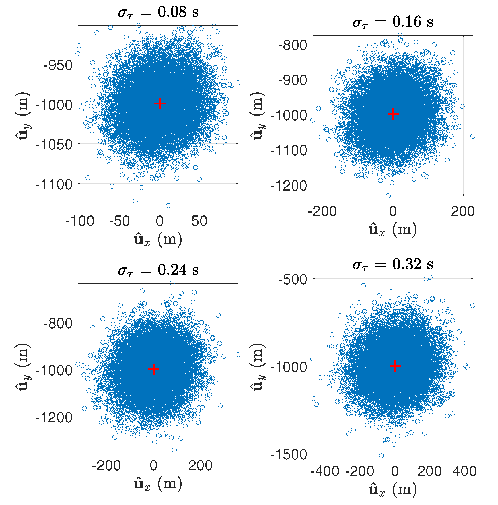
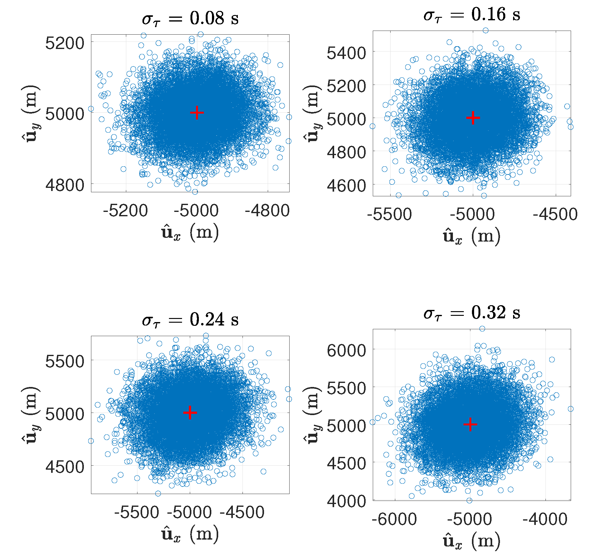
• We cautiously verify the deployability of the algorithm by setting the measurement noise levels far higher than what can be achieved by real systems. Simulation experiments with extreme parameter settings are alternative to the costly field tests.

The rest of this paper is organized as follows. Section 2 provides the location scenario and its observation model. Section 3 performs the CRB analysis for the elliptical location problem. Section 4 presents the SDP-based location algorithm and its complexity analysis. Section 5 contains the simulation results and compares our algorithm with state-of-the-art ones, and Section 6 draws conclusions.

We shall use bold uppercase letter to denote a matrix and bold lowercase letter to denote a vector. The notation $\mathbf{M}⪰\mathbf{0}$ means that $\mathbf{M}$ is a positive semidefinite matrix, and $\mathbf{v}\ge \mathbf{0}$ means that each element of $\mathbf{v}$ is non-negative. ${\mathbf{1}}_{p\times q}$ is a $p\times q$ ones matrix, and ${\mathbf{I}}_p$ is an identity matrix of size p. The symbol ⊗ is the Kronecker product operator. $\parallel \mathbf{v}\parallel$ is the Euclidean norm of $\mathbf{v}$. $cond\left(\mathbf{M}\right)$ is the condition number of $\mathbf{M}$. $diag\left(\mathbf{v}\right)$ is the square diagonal matrix with the elements of vector $\mathbf{v}$ on the main diagonal. $\mathbf{B}=blkdiag({\mathbf{M}}_1,\dots ,{\mathbf{M}}_N)$ is the block diagonal matrix created by aligning the matrices ${\mathbf{M}}_1,\dots ,{\mathbf{M}}_N$ along the diagonal of $\mathbf{B}$. If $\mathbf{X}$ and $\mathbf{Y}$ are symmetric, then $\langle \mathbf{X},\mathbf{Y}\rangle$ is a Frobenius inner product of $\mathbf{X}$ and $\mathbf{Y}$. We use ${\rho }_{\mathbf{x},\mathbf{y}}$ as a shorthand for $(\mathbf{x}-\mathbf{y})/\parallel \mathbf{x}-\mathbf{y}\parallel$.

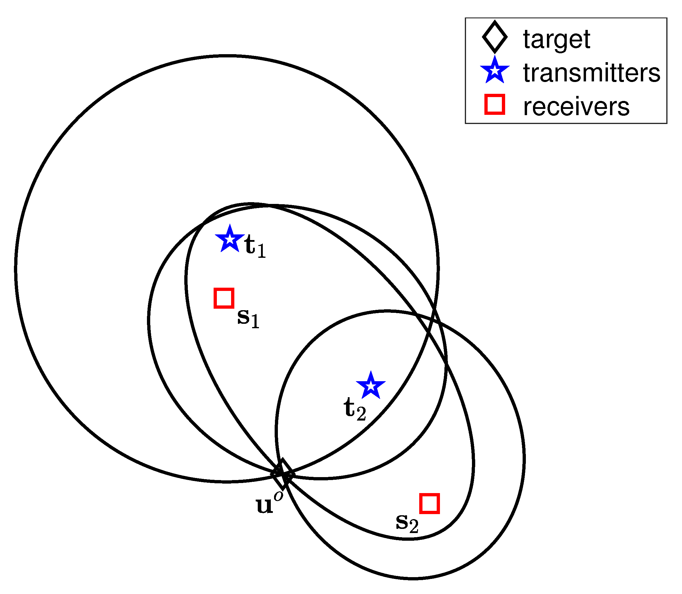
2. Problem Formulation and Data Model

We are interested in a d-dimensional ($d=2$ or $d=3$) elliptical location scenario where the transmitters and receivers are stationary. Let M be the number of transmitters and N be the number of receivers. The position vectors of transmitters and receivers are ${\mathbf{t}}_i$ and ${\mathbf{s}}_j$, for $i=1,2,\dots ,M$ and $j=1,2,\dots ,N$, which are available in practice. Let c be the known signal propagation speed. The unknown position vector of the target of concern is denoted by ${\mathbf{u}}^o$. A typical location scenario for a two-dimensional case is illustrated in Figure 1. The equations of the ellipses in Figure 1 are shown in Equation (1). The target is located at the intersection of these ellipses.

The transmitter at ${\mathbf{t}}_i$ radiates a signal and the receiver at ${\mathbf{s}}_j$ observes the signal from direct propagation (from ${\mathbf{t}}_i$ to ${\mathbf{s}}_j$) and from indirect reflection of the target at ${\mathbf{u}}^o$ (from ${\mathbf{t}}_i$ to ${\mathbf{u}}^o$ and then from ${\mathbf{u}}^o$ to ${\mathbf{s}}_j$). The ideal differential TOA measurement between the indirect path and direct path is

$${\tau }_{i,j}^o=\frac{1}{c}\left(\parallel {\mathbf{u}}^o-{\mathbf{t}}_i\parallel +\parallel {\mathbf{u}}^o-{\mathbf{s}}_j\parallel -\parallel {\mathbf{t}}_i-{\mathbf{s}}_j\parallel \right),i=1,2,\dots ,M,j=1,2,\dots ,N.$$

(1)

Obviously, the graph of ${\mathbf{u}}^o$ is an ellipse with foci ${\mathbf{t}}_i$ and ${\mathbf{s}}_j$ for each pair of i and j.

In an actual elliptical location system, we have the measurements

$${\tau }_{i,j}={\tau }_{i,j}^o+n_{i,j},i=1,2,\dots ,M,j=1,2,\dots ,N,$$

(2)

where $n_{i,j}$ is the measurement noise. For notation simplicity, we collect ${\tau }_{i,j}$ to form a measurement vector. For the transmitter at ${\mathbf{t}}_i(i=1,2,\dots ,M)$, all the related measurements can be collected in a column vector ${\tau }_i={[{\tau }_{i,1},{\tau }_{i,2},\dots ,{\tau }_{i,N}]}^{\mathrm{T}}$. Further, the measurements related to all the transmitters can be denoted as $\tau ={[{\tau }_1^{\mathrm{T}},{\tau }_2^{\mathrm{T}},\cdots ,{\tau }_M^{\mathrm{T}}]}^{\mathrm{T}}$. It is customary to assume that

$${\tau }_i\sim \mathcal{N}({\tau }_i^o,{\mathbf{Q}}_{{\tau }_i}),i=1,2,\dots ,M,$$

(3)

where ${\tau }_i^o$ is the mean vector of ${\tau }_i$ and ${\mathbf{Q}}_{{\tau }_i}$ is a known covariance matrix of ${\tau }_i$ [28]. Furthermore,

$$\tau \sim \mathcal{N}(\mathbf{m},\mathbf{V}),$$

(4)

where $\mathbf{m}={[{{\tau }_1^o}^{\mathrm{T}},{{\tau }_2^o}^{\mathrm{T}},\cdots ,{{\tau }_M^o}^{\mathrm{T}}]}^{\mathrm{T}}$ is the mean vector of $\tau$ and $\mathbf{V}$ is the covariance matrix of $\tau$. $\mathbf{V}=blkdiag({\mathbf{Q}}_{{\tau }_1},{\mathbf{Q}}_{{\tau }_2},\dots ,{\mathbf{Q}}_{{\tau }_M})$ if we further assume that the measurements across distinct transmitters are uncorrelated. So far we get the overall data model of (4) for AEL. Omitting the term $\parallel {\mathbf{t}}_i-{\mathbf{s}}_j\parallel$ in (1) yields the data model for SEL. The problem we are facing is to design, implement and evaluate an estimator for the unknown target position vector ${\mathbf{u}}^o$ in the data model.

3. Cramér–Rao Bound

We now give the CRB for the estimation problem proposed in Section 2. The CRB can serve as the benchmark for our proposed estimator in Section 4. The CRB gives a lower bound for the mean square error (MSE) matrix of an unbiased estimator of unknown parameter vector ${\mathbf{u}}^o$ [61]. The square root of the trace of CRB matrix has the physical meaning that it is the minimum possible root-mean-square error (RMSE) for positioning the target unbiasedly. Evaluation of CRB is very useful because it not only gives us a performance benchmark, but also provides us insight into the system design.

Because the observation model (4) is a Gaussian model, it is easy to get the CRB for the estimation of ${\mathbf{u}}^o$ as follows [61].

$$CRB={\left[{\left(\frac{\partial \mathbf{m}}{\partial {\mathbf{u}}^o}\right)}^{\mathrm{T}}{\mathbf{V}}^{-1}\frac{\partial \mathbf{m}}{\partial {\mathbf{u}}^o}\right]}^{-1}.$$

(5)

For numerical computation using (5), $\partial \mathbf{m}/\partial {\mathbf{u}}^o$ is needed. The details are given below.

$$\frac{\partial \mathbf{m}}{\partial {\mathbf{u}}^o}=\left[\begin{array}{c}\partial {\tau }_1^o/\partial {\mathbf{u}}^o\\ \partial {\tau }_2^o/\partial {\mathbf{u}}^o\\ ⋮\\ \partial {\tau }_M^o/\partial {\mathbf{u}}^o\end{array}\right],$$

(6)

where

$$\begin{array}{lll}\frac{\partial {\tau }_i^o}{\partial {\mathbf{u}}^o}& =& {\left[\begin{array}{c}{\left(\frac{\partial {\tau }_{i,1}^o}{\partial {\mathbf{u}}^o}\right)}^{\mathrm{T}},{\left(\frac{\partial {\tau }_{i,2}^o}{\partial {\mathbf{u}}^o}\right)}^{\mathrm{T}},\dots ,{\left(\frac{\partial {\tau }_{i,N}^o}{\partial {\mathbf{u}}^o}\right)}^{\mathrm{T}}\end{array}\right]}^{\mathrm{T}},\\ \frac{\partial {\tau }_{i,j}^o}{\partial {\mathbf{u}}^o}& =& \frac{1}{c}{\left({\rho }_{{\mathbf{u}}^o,{\mathbf{t}}_i}+{\rho }_{{\mathbf{u}}^o,{\mathbf{s}}_j}\right)}^{\mathrm{T}},\end{array}$$

for $i=1,2,\dots ,M$ and $j=1,2,\dots ,N$.

4. Design of the Estimator

Maximum likelihood estimation is overwhelmingly the most popular approach to obtaining practical estimators. Our design procedure of MLE based on semidefinite relaxation (SDR) technique is divided into three steps. We first establish a quadratic optimization problem with multiple quadratic equality/inequality constraints based on the maximum likelihood criterion. In the second step we rewrite the quadratic optimization problem using Frobenius inner product. Finally, we drop the nonconvex constraints in the problem.

4.1. Formulation of MLE as a Quadratic Optimization Problem

Under the Gaussian noise assumption in (4) and with the matrix reformulation of (1), the NLL function of the estimation problem is

$$\ell \left(\mathbf{u}\right)={(\mathbf{A}\mathbf{x}-\mathbf{b})}^{\mathrm{T}}{\mathbf{V}}^{-1}(\mathbf{A}\mathbf{x}-\mathbf{b})+{\xi }_1,$$

(7)

where

$${\mathbf{v}}_i=\frac{1}{c}{\left[\parallel {\mathbf{z}}_i-{\mathbf{z}}_{M+1}\parallel ,\dots ,\parallel {\mathbf{z}}_i-{\mathbf{z}}_{M+N}\parallel \right]}^{\mathrm{T}},i=1,2,\dots ,M,$$

$$\mathbf{x}=\frac{1}{c}{[\parallel \mathbf{u}-{\mathbf{z}}_1\parallel ,\parallel \mathbf{u}-{\mathbf{z}}_2\parallel ,\dots ,\parallel \mathbf{u}-{\mathbf{z}}_{M+N}\parallel ]}^{\mathrm{T}},$$

$$\mathbf{A}=[{\mathbf{I}}_M\otimes {\mathbf{1}}_{N\times 1},{\mathbf{1}}_{M\times 1}\otimes {\mathbf{I}}_N],$$

$$\mathbf{v}={[{\mathbf{v}}_1^{\mathrm{T}},{\mathbf{v}}_2^{\mathrm{T}},\dots ,{\mathbf{v}}_M^{\mathrm{T}}]}^{\mathrm{T}},$$

$$\mathbf{b}=\mathbf{v}+\tau .$$

In (7), $\mathbf{u}$ is the optimization variable and ${\xi }_1$ does not depend on $\mathbf{u}$. Here we write ${\mathbf{z}}_i={\mathbf{t}}_i$ for $i=1,2,\dots ,M$ and ${\mathbf{z}}_i={\mathbf{s}}_{i-M}$ for $i=M+1,M+2,\dots ,M+N$. The NLL function is nonconvex with respect to the optimization variable $\mathbf{u}$.

In the MLE sense, by introducing auxiliary optimization variable $\mathbf{x}$, the estimator can be considered as the optimal solution of the constrained optimization problem as below.

$$\begin{array}{cccc}\hfill & {\mathrm{minimize}}_{\mathbf{u},\mathbf{x}}\hfill & \hfill & {(\mathbf{A}\mathbf{x}-\mathbf{b})}^{\mathrm{T}}{\mathbf{V}}^{-1}(\mathbf{A}\mathbf{x}-\mathbf{b}),\hfill \end{array}$$

(8a)

$$\begin{array}{cccc}\hfill & \mathrm{subject}\mathrm{to}\hfill & \hfill & \mathbf{x}=\frac{1}{c}{[\parallel \mathbf{u}-{\mathbf{z}}_1\parallel ,\parallel \mathbf{u}-{\mathbf{z}}_2\parallel ,\dots ,\parallel \mathbf{u}-{\mathbf{z}}_{M+N}\parallel ]}^{\mathrm{T}}.\hfill \end{array}$$

(8b)

The objective function (8a) can be expanded as

$${\mathbf{x}}^{\mathrm{T}}{\mathbf{A}}^{\mathrm{T}}{\mathbf{V}}^{-1}\mathbf{A}\mathbf{x}-2{\mathbf{b}}^{\mathrm{T}}{\mathbf{V}}^{-1}\mathbf{A}\mathbf{x}+{\xi }_2,$$

where ${\xi }_2={\mathbf{b}}^{\mathrm{T}}{\mathbf{V}}^{-1}\mathbf{b}$ is a constant. Then the original problem (8) can be rewritten as follows.

$$\begin{array}{cccc}\hfill & {\mathrm{minimize}}_{\mathbf{u},\mathbf{x}}\hfill & \hfill & {\mathbf{x}}^{\mathrm{T}}{\mathbf{A}}^{\mathrm{T}}{\mathbf{V}}^{-1}\mathbf{A}\mathbf{x}-2{\mathbf{b}}^{\mathrm{T}}{\mathbf{V}}^{-1}\mathbf{A}\mathbf{x},\hfill \end{array}$$

(9a)

$$\begin{array}{cccc}\hfill & \mathrm{subject}\mathrm{to}\hfill & \hfill & \mathbf{x}=\frac{1}{c}{[\parallel \mathbf{u}-{\mathbf{z}}_1\parallel ,\parallel \mathbf{u}-{\mathbf{z}}_2\parallel ,\dots ,\parallel \mathbf{u}-{\mathbf{z}}_{M+N}\parallel ]}^{\mathrm{T}}.\hfill \end{array}$$

(9b)

It is ready to recognize the problem (9) as a quadratic optimization problem with multiple quadratic equality constraints [38,62]. While the objective function (9a) is convex, the constraint functions (9b) are nonconvex. In short, the MLE involves a nonconvex optimization problem. It is well known that computing the MLE via a grid search results in computationally prohibitive solutions and Gauss-Newton implementation of the MLE requires carefully chosen initial guesses [61]. For such a computationally difficult problem, our strategy is to approximate the problem (9) to a convex one using SDR technique. The related SDP can be solved in a polynomial complexity using interior-point methods without causing the risk of local convergence [63,64].

4.2. Some Equivalent Transformation

In order to introduce semidefinite constraints, some necessary equality transformations are made in this subsection. Rewriting the objective function (9a) in matrix form and reformulating the constraints (9b), the problem (9) is recast as

$$\begin{array}{cccc}\hfill & {\mathrm{minimize}}_{\mathbf{u},\mathbf{x}}\hfill & \hfill & \left[\begin{array}{cc}{\mathbf{x}}^{\mathrm{T}}& 1\end{array}\right]\mathbf{F}{\left[\begin{array}{cc}{\mathbf{x}}^{\mathrm{T}}& 1\end{array}\right]}^{\mathrm{T}},\hfill \end{array}$$

(10a)

$$\begin{array}{cccc}\hfill & \mathrm{subject}\mathrm{to}\hfill & \hfill & x_i\ge 0,i=1,2,\dots ,M+N,\hfill \end{array}$$

(10b)

$$\begin{array}{ccc}\hfill & \hfill & x_i^2=\frac{1}{c^2}\left[\begin{array}{cc}{\mathbf{u}}^{\mathrm{T}}& 1\end{array}\right]{\mathbf{G}}_i{\left[\begin{array}{cc}{\mathbf{u}}^{\mathrm{T}}& 1\end{array}\right]}^{\mathrm{T}},i=1,2,\dots ,M+N,\hfill \end{array}$$

(10c)

where

$$\begin{array}{lll}\mathbf{F}& =& \left[\begin{array}{cc}{\mathbf{A}}^{\mathrm{T}}{\mathbf{V}}^{-1}\mathbf{A}& -{\mathbf{A}}^{\mathrm{T}}{\mathbf{V}}^{-\mathrm{T}}\mathbf{b}\\ -{\mathbf{b}}^{\mathrm{T}}{\mathbf{V}}^{-1}\mathbf{A}& 0\end{array}\right],\\ {\mathbf{G}}_i& =& \left[\begin{array}{cc}{\mathbf{I}}_d& -{\mathbf{z}}_i\\ -{\mathbf{z}}_i^{\mathrm{T}}& \parallel {\mathbf{z}}_i{\parallel }^2\end{array}\right],i=1,2,\dots ,M+N.\end{array}$$

(11)

Note that the parameter matrices $\mathbf{F}$ and ${\mathbf{G}}_i$ are positive semidefinite. Then we introduce two new matrix variables $\mathbf{U}$ and $\mathbf{X}$, reformulating the problem (10) as

$$\begin{array}{cccc}\hfill & {\mathrm{minimize}}_{\mathbf{u},\mathbf{x},\mathbf{U},\mathbf{X}}\hfill & \hfill & \langle \mathbf{F},\tilde{\mathbf{X}}\rangle ,\hfill \end{array}$$

(12a)

$$\begin{array}{cccc}\hfill & \mathrm{subject}\mathrm{to}\hfill & \hfill & \mathbf{U}=\mathbf{u}{\mathbf{u}}^{\mathrm{T}},\hfill \end{array}$$

(12b)

$$\begin{array}{ccc}\hfill & \hfill & \mathbf{X}=\mathbf{x}{\mathbf{x}}^{\mathrm{T}},\hfill \end{array}$$

(12c)

$$\begin{array}{ccc}\hfill & \hfill & x_i\ge 0,i=1,2,\dots ,M+N,\hfill \end{array}$$

(12d)

$$\begin{array}{ccc}\hfill & \hfill & X_{i,i}=\frac{1}{c^2}\langle {\mathbf{G}}_i,\tilde{\mathbf{U}}\rangle ,i=1,2,\dots ,M+N,\hfill \end{array}$$

(12e)

where

$$\tilde{\mathbf{X}}=\left[\begin{array}{cc}\mathbf{X}& \mathbf{x}\\ {\mathbf{x}}^{\mathrm{T}}& 1\end{array}\right],\tilde{\mathbf{U}}=\left[\begin{array}{cc}\mathbf{U}& \mathbf{u}\\ {\mathbf{u}}^{\mathrm{T}}& 1\end{array}\right].$$

(13)

We emphasize that by now the problem (12) is still equivalent to the original MLE problem (8), but not a convex one.

4.3. Semidefinite Relaxation

In this subsection, we relax the problem (12) to an SDP problem. The semidefinite programs can be solved almost as easily as linear programs with interior-point methods [64] and several advanced SDP solvers are readily available [65]. By the Schur complement condition for positive semidefiniteness [66],

$$\begin{array}{ccc}\hfill \mathbf{U}=\mathbf{u}{\mathbf{u}}^{\mathrm{T}}& \iff & \tilde{\mathbf{U}}⪰\mathbf{0}\mathrm{has}\mathrm{rank}1,\hfill \end{array}$$

(14)

$$\begin{array}{ccc}\hfill \mathbf{X}=\mathbf{x}{\mathbf{x}}^{\mathrm{T}}& \iff & \tilde{\mathbf{X}}⪰\mathbf{0}\mathrm{has}\mathrm{rank}1.\hfill \end{array}$$

(15)

In view of (14) and (15), if the constraints (12b) and (12c) in (12) are relaxed to drop the (nonconvex) rank-one constraints, then we obtain the following (convex) SDR problem.

$$\begin{array}{cccc}\hfill & {\mathrm{minimize}}_{\mathbf{Z}}\hfill & \hfill & \langle \mathbf{F},\tilde{\mathbf{X}}\rangle ,\hfill \end{array}$$

(16a)

$$\begin{array}{cccc}\hfill & \mathrm{subject}\mathrm{to}\hfill & \hfill & \tilde{\mathbf{U}}⪰0,\tilde{\mathbf{X}}⪰0,\mathbf{x}\ge 0,\hfill \end{array}$$

(16b)

$$\begin{array}{ccc}\hfill & \hfill & {\tilde{\mathbf{U}}}_{d+1,d+1}=1,{\tilde{\mathbf{X}}}_{M+N+1,M+N+1}=1,\hfill \end{array}$$

(16c)

$$\begin{array}{ccc}\hfill & \hfill & {\tilde{\mathbf{X}}}_{M+N+1,i}=x_i,i=1,2,\dots ,M+N,\hfill \end{array}$$

(16d)

$$\begin{array}{ccc}\hfill & \hfill & {\tilde{\mathbf{X}}}_{i,i}=\frac{1}{c^2}\langle {\mathbf{G}}_i\tilde{\mathbf{U}}\rangle ,i=1,2,\dots ,M+N,\hfill \end{array}$$

(16e)

where $\mathbf{Z}=blkdiag(\tilde{\mathbf{X}},\tilde{\mathbf{U}},diag\left(\mathbf{x}\right))$ is the primal variable.

Now note that the problem (16) is an approximation of the original problem (8), but a more tractable one. We call the minimizer (if unique) of the SDP problem (16) as an SDR solution to the original elliptical location problem.

4.4. Semidefinite Programming Solver

In order to design an efficient numerical optimization algorithm, we first find the dual problem of the primal problem (16). By the conic duality theorem [41], the dual of problem (16) is as follows.

$$\begin{array}{cccc}\hfill & {\mathrm{maximize}}_{\mathbf{S},\mathbf{y}}\hfill & \hfill & y_1+y_2,\hfill \end{array}$$

(17a)

$$\begin{array}{cccc}\hfill & \mathrm{subject}\mathrm{to}\hfill & \hfill & \left[\begin{array}{cc}-c^{2}diag\left(\beta \right)& \alpha /2\\ {\alpha }^{\mathrm{T}}/2& y_1\end{array}\right]+{\mathbf{S}}_1=\mathbf{F},\hfill \end{array}$$

(17b)

$$\begin{array}{ccc}\hfill & \hfill & \left[\begin{array}{cc}{\mathbf{0}}_{d\times d}& \mathbf{0}\\ {\mathbf{0}}^{\mathrm{T}}& y_2\end{array}\right]+\sum _{i=1}^{M+N}{\beta }_i{\mathbf{G}}_i+{\mathbf{S}}_2=\mathbf{0},\hfill \end{array}$$

(17c)

$$\begin{array}{ccc}\hfill & \hfill & -\alpha +\mathbf{s}=\mathbf{0},\hfill \end{array}$$

(17d)

$$\begin{array}{ccc}\hfill & \hfill & \mathbf{S}⪰\mathbf{0},\hfill \end{array}$$

(17e)

where $\mathbf{y}={[y_1,y_2,{\alpha }^{\mathrm{T}},{\beta }^{\mathrm{T}}]}^{\mathrm{T}}$ and $\mathbf{S}=blkdiag({\mathbf{S}}_1,{\mathbf{S}}_2,diag\left(\mathbf{s}\right))$ are the dual variables. The lengths of vectors $\alpha$ and $\beta$ are both $(M+N)$.

From the perspective of optimization theory, the rest of the work is to reduce the duality gap of primal-dual problem pairs (16) and (17) to find the optimal solution. We will solve the primal-dual problem pairs with an interior-point primal-dual path-following method.

To develop efficient interior-point algorithms, the key is to find suitable barrier functions. With an appropriate choice of barrier functions, the interior-point algorithm admits a polynomial time implementation. We choose the canonical barrier functions for our problems (16) and (17), and then the parameter of barrier is $n=2(M+N+1)+d$ [41]. The barrier functions are added to the objective functions, forming primal and dual barrier problems. Given a barrier weight parameter $\mu >0$, the central path associated with these barrier problems is defined as the set of points

$$C_{\mathrm{SDP}}\left(\mu \right)=\left\{(\mathbf{Z},\mathbf{S},\mathbf{y})\mathrm{strictly}\mathrm{feasible}\mathrm{in}\right(16\left)\mathrm{and}\right(17)\mid \mathbf{Z}\mathbf{S}=\mu \mathbf{I}\},\mu >0.$$

(18)

Now all we need for obtaining good primal and dual approximate solutions is to trace fast the central path (18). In practice, path following (i.e., computing primal-dual search directions) can be implemented in a moderate (few tens) number of iterations, each iteration reducing to assembling and solving a Newton system of linear equations resulted from linearization of (19) below.

$$\left\{\begin{array}{cc}\hfill & \mathrm{the}\mathrm{equality}\mathrm{constraints}\mathrm{in}\mathrm{the}\mathrm{primal}\mathrm{problem}(16)\hfill \\ \hfill & \mathrm{the}\mathrm{equality}\mathrm{constraints}\mathrm{in}\mathrm{the}\mathrm{dual}\mathrm{problem}(17)\hfill \\ \hfill & \mathbf{Z}\mathbf{S}=\mu \mathbf{I}\hfill \\ \hfill & \mathbf{Z}\succ \mathbf{0},\mathbf{S}\succ \mathbf{0}.\hfill \end{array}\right.$$

(19)

In summary, our algorithm is shown in Algorithm 1, where $({\mathbf{Z}}^0,{\mathbf{S}}^0,{\mathbf{y}}^0)$ are the initial values of primal and dual variables, and $ϵ>0$ is a tolerance parameter for balancing the accuracy and speed. One advantage of using SDR technique is that the convergence of the algorithm is guaranteed, regardless of the initial values.

Algorithm 1 Primal-dual path-following interior-point method.

1: procedurePD-PF-IP( ${\mathbf{Z}}^0,{\mathbf{S}}^0,{\mathbf{y}}^0,ϵ>0$ ) 2:     $\mathbf{Z}\leftarrow {\mathbf{Z}}^0,\mathbf{S}\leftarrow {\mathbf{S}}^0,\mathbf{y}\leftarrow {\mathbf{y}}^0$ 3:     $\mu \leftarrow \langle \mathbf{Z},\mathbf{S}\rangle /n$ 4:     while $\langle \mathbf{Z},\mathbf{S}\rangle >ϵ$ do 5:         Compute primal-dual search directions $\Delta \mathbf{y}$, $\Delta \mathbf{S}$ and $\Delta \mathbf{Z}$ using Newton’s method on (19) 6:         $\mathbf{Z}\leftarrow \mathbf{Z}+\Delta \mathbf{Z},\mathbf{S}\leftarrow \mathbf{S}+\Delta \mathbf{S},\mathbf{y}\leftarrow \mathbf{y}+\Delta \mathbf{y},\mu \leftarrow \langle \mathbf{Z},\mathbf{S}\rangle /n$ 7:     end while 8: end procedure

Using (13), the minimizer of (16) (i.e., the SDR solution) contains an estimate of target location ${\mathbf{u}}^o$. Strictly speaking, if $rank(\tilde{\mathbf{X}})=rank(\tilde{\mathbf{U}})=1$ holds, we do not need to further refine the SDR solution. Otherwise, some post-processing techniques are required to improve the accuracy of the estimate [45]. Fortunately, our experiments in Section 5 show that our algorithms require little post-processing.

4.5. Complexity Analysis

Now we give a complexity analysis to show that our algorithm complexity is controllable as the numbers of transmitters and receivers increase. Since our estimator is implemented using the interior-point method, its complexity analysis can be based on some established theoretical results [40,41]. The worst-case Newton complexity of an interior-point primal-dual path-following method is $O\left(1\right)n^{\frac{1}{2}}ln\frac{1}{ϵ}$.

We should also know how heavy a Newton step is, i.e., what is its arithmetic cost of each iteration. We count the numbers of semidefinite matrix blocks and equality constraints in the SDP problem (16). In total, there is one semidefinite matrix block of size $(M+N+1)$, one semidefinite matrix block of size $(d+1)$, and $(M+N)$ non-negative scalar variables. Furthermore, there are $2(M+N+1)$ equality constraints on these matrix/scalar variables. When $(M+N+1)\gg d$, the flop count in each Newton step is approximately $6{(M+N+1)}^4$.

In conclusion, the total complexity of our algorithm is on the order of ${(M+N+1)}^{4.5}ln\frac{1}{ϵ}$.

5. Results and Discussion

We conducted a series of Monte Carlo simulations to evaluate the proposed SDR estimator comprehensively. Generally, when using convex relaxation techniques for parameter estimation, three aspects of the estimator are of concern: What is the statistical performance of the estimator, What is the degree of relaxation of the related optimization model, and whether the relaxed solution needs post-processing.

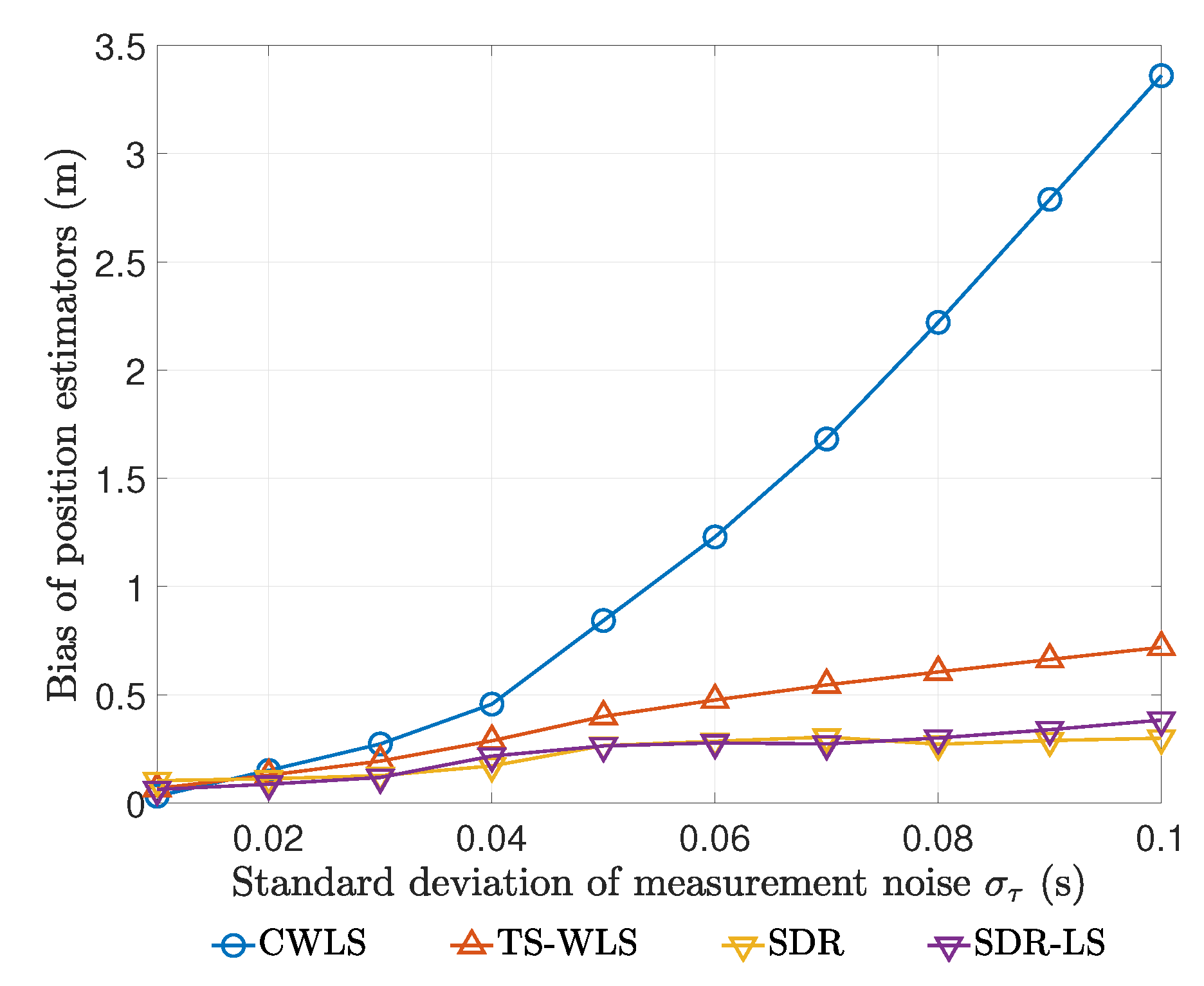
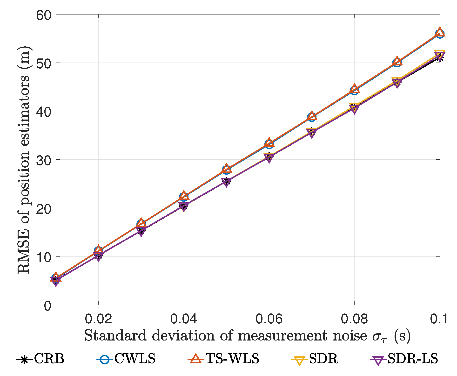
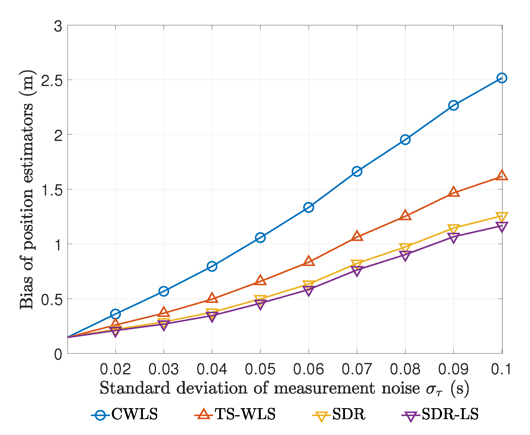
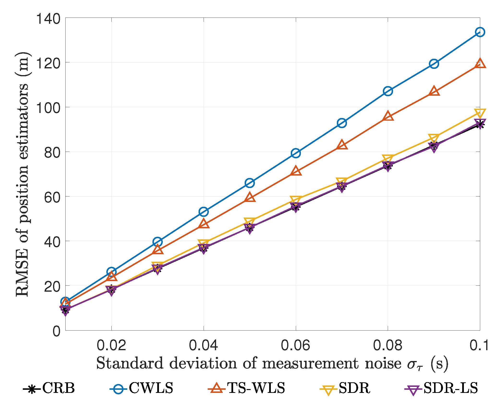
• To ascertain the statistical performance of the proposed SDR estimator, we compared it with several closed-form methods recently proposed, i.e., Yang’s TS-WLS method [21] and Amiri’s CWLS method [20]. For a given estimator $\widehat{\mathbf{u}}$ of the unknown parameter ${\mathbf{u}}^o$, its performance is measured by the empirical bias and RMSE, which are defined as follows.

  $$\begin{array}{lll}\mathrm{bias}& =& ∥\frac{1}{L}\sum _{\ell =1}^L{\mathbf{u}}_{\ell }-{\mathbf{u}}^o∥,\\ \mathrm{RMSE}& =& \sqrt{\frac{1}{L}\left(\sum _{\ell =1}^L{\parallel {\mathbf{u}}_{\ell }-{\mathbf{u}}^o\parallel }^2\right)},\end{array}$$

  where L is the number of Monte Carlo simulations and ${\mathbf{u}}_{\ell }$ is the ℓ-th random realization of $\widehat{\mathbf{u}}$. In our following experiments, we set $L={10}^4$ and compared the biases and RMSEs of all these estimators at different noise levels.
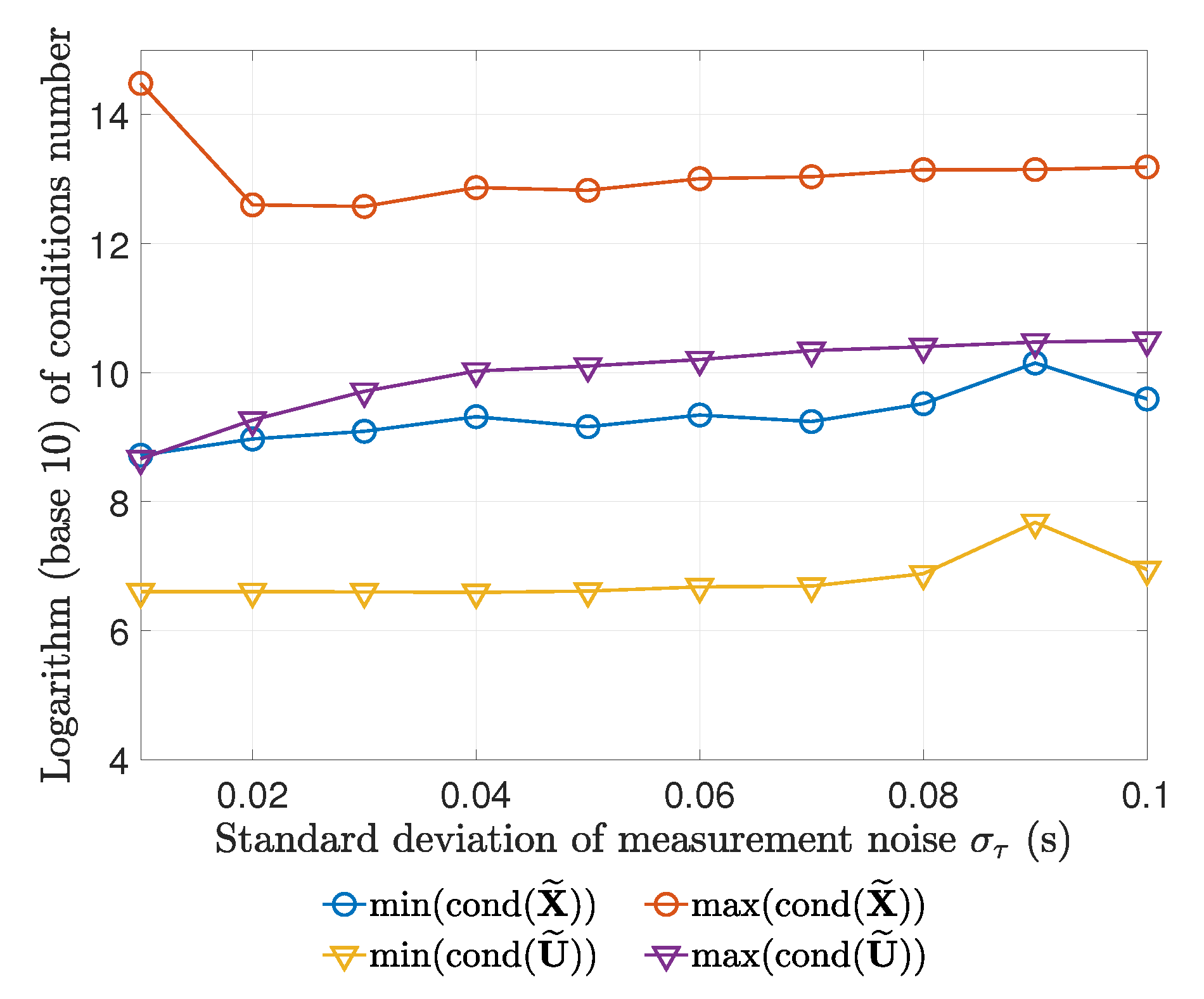
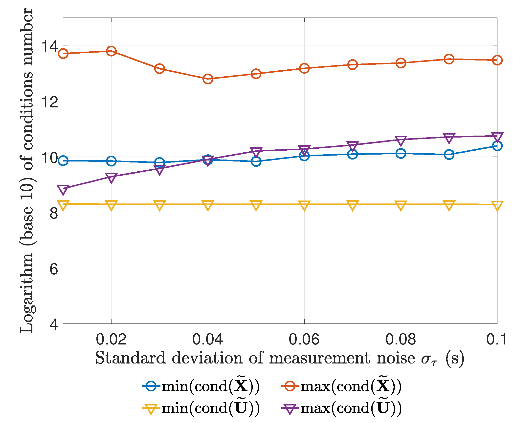
• To measure the tightness of the relaxed optimization model in (16), we recorded the condition numbers of the optimal solutions of $\tilde{\mathbf{X}}$ and $\tilde{\mathbf{U}}$ in (17) at different noise levels. The motivation is that if the condition number of a matrix is greater than ${10}^4$, then it can be approximated as a rank-1 matrix [44].
• To verify whether the SDR solution needs post-processing, we checked the performance improvement gifted by post-processing using local search under different noise conditions. We used the SDR solution as the initial point for the commercial optimization solver MATLAB function lsqnonlin, and the algorithm for lsqnonlin was set as ‘trust-region-reflective‘. Our estimator with post-processing is simply referred to as SDR-LS.

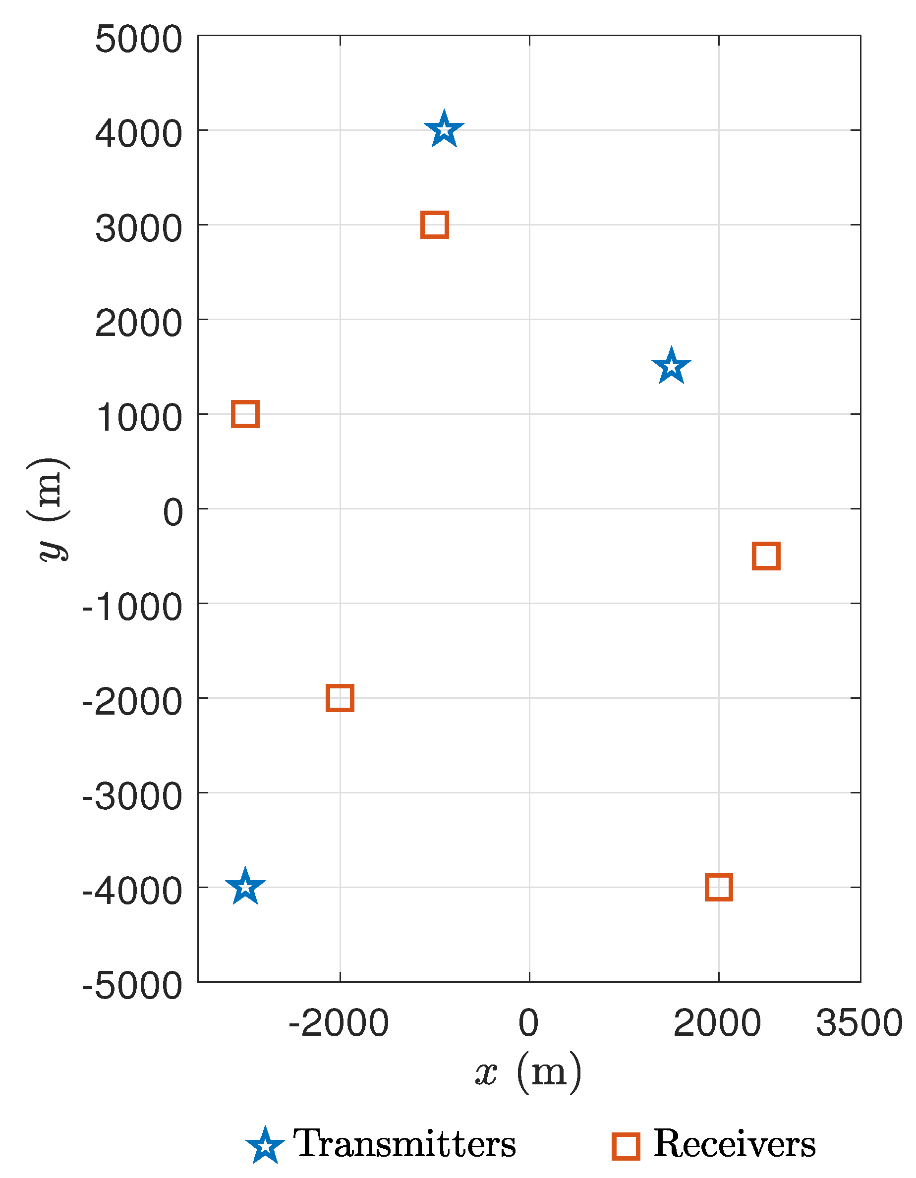
5.1. Localization Scenarios

Our experimental design was as follows. We used $M=3$ transmitters and $N=5$ receivers to determine the position ${\mathbf{u}}^o$ of a stationary object. Their positions are given in

Table 1. Positions of transmitters and receivers in Monte Carlo experiments.

Transmitter/Receiver No.	Position Coordinates (m)
${\mathbf{t}}_1$	${[1500,1500]}^{\mathrm{T}}$
${\mathbf{t}}_2$	${[-900,4000]}^{\mathrm{T}}$
${\mathbf{t}}_3$	${[-3000,-4000]}^{\mathrm{T}}$
${\mathbf{s}}_1$	${[-1000,3000]}^{\mathrm{T}}$
${\mathbf{s}}_2$	${[2500,-500]}^{\mathrm{T}}$
${\mathbf{s}}_3$	${[-3000,1000]}^{\mathrm{T}}$
${\mathbf{s}}_4$	${[2000,-4000]}^{\mathrm{T}}$
${\mathbf{s}}_5$	${[-2000,-2000]}^{\mathrm{T}}$

.

The location geometry was the same as the one in [22] and depicted in Figure 2.

The signal propagation speed was $c=1500$ m/s. The covariance matrix of the observation vector ${\tau }_i$ related to the i-th transmitter was ${\mathbf{Q}}_{{\tau }_i}={\sigma }_{\tau }^2\mathbf{R}$ for $i=1,2,\dots ,M$, where ${\sigma }_{\tau }$ was a given positive constant, and $\mathbf{R}=\frac{1}{2}({\mathbf{1}}_{N\times N}+{\mathbf{I}}_N)$ [34].

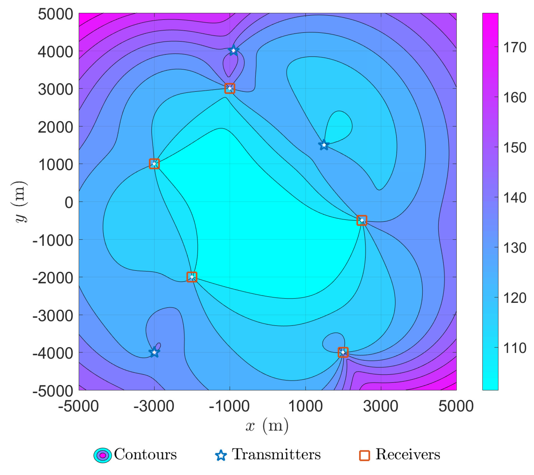
5.2. Visualization of Cramér–Rao Bound and Selection of Testing Points

We visualized the CRB given by (5), which sets a lower bound for the MSE of our estimation problem proposed in Section 2. We selected two representative positions as test points according to the square root of the trace of CRB matrix. Based on these considerations, we plotted the contours of the square root of the trace of CRB matrix for ${\sigma }_{\tau }=0.2$ as in Figure 3.

The positioning difficulty of the target at different locations indicated by the contours in Figure 3 is consistent with our intuitive experience. According to the contours, we selected easier point $[0,-1000]$ m (with the minimum square root of trace of CRB matrix) and harder point $[-5000,5000]$ m (with the maximum square root of trace of CRB matrix) as the two representative test points for further in-depth comparative study in next subsection.

5.3. Results on the Two Representative Test Points

In order to examine the performance of various algorithms at different noise levels, we increased measurement noise level ${\sigma }_{\tau }$ from $0.01$ s to $0.1$ s with a step size of $0.01$ s in the following simulation experiments.

5.3.1. Results on Easier Test Point

For this easier test point ${\mathbf{u}}^o={[0,-1000]}^{\mathrm{T}}$ m, the biases and RMSEs produced by different estimators at different noise levels are shown in Figure 4 and Figure 5.

It can be seen that when the noise level increases, there is a sharp increase in the bias of CWLS estimator, while the other three algorithms control the bias very well over a wide range of noise levels. Furthermore, a closer look at Figure 4 reveals that the bias of TS-WLS estimator is still moderately larger than that of SDR estimator and SDR-LS estimator. We believe that these findings are due to the following two facts. First, the square terms of observation errors are ignored in the models of CWLS estimator and TS-WLS estimator. In addition, CWLS estimator involves solving high-order polynomial equations with numerical instability.

Due to their excellent biases, we limited our attention to SDR estimator and SDR-LS estimator. Figure 5 shows that the RMSEs of both SDR estimator and SDR-LS estimator agree well with CRBs at all noise levels. This implies that our SDR estimator has achieved the theoretically optimal RMSE performance at this test point and it does not need to use local search for post-processing.

To further confirm that the SDR model is tight enough, we showed the maxima and minima of the condition numbers of optimal $\tilde{\mathbf{X}}$ and $\tilde{\mathbf{U}}$ in the Monte Carlo experiments at different noise levels in Figure 6. As can be seen, the condition numbers are much larger than the critical value of ${10}^4$ proposed by [44].

As a practical guideline for deploying our SDR estimator in actual systems, we drew the scatter plots of its Monte Carlo random realizations at even higher noise levels in Figure 7. It can be seen that, no matter how high the noise level is, the average value of a huge large number of estimation results is highly consistent with the actual coordinates of the target.

5.3.2. Results on Harder Test Point

For this harder test point ${\mathbf{u}}^o={[-5000,5000]}^{\mathrm{T}}$ m, the biases and RMSEs produced by different estimators at different noise levels are shown in Figure 8 and Figure 9.

As shown in Figure 8, the bias of SDR-LS estimator is the smallest, and that of CWLS estimator is the largest. What is worth noting in Figure 8 is that at all noise levels, SDR estimator’s bias is slightly larger than that of SDR-LS estimator. Furthermore, a similar situation was observed when we examined the RMSEs in Figure 9. It must be pointed out that SDR-LS estimator’s RMSE agrees well with CRB here. These results suggest that SDR estimator provides a reliable initial solution for local search, and local search based on this initial solution achieves theoretically optimal performance. Since SDR estimator is near optimal, we suggest that the practitioners decide whether post-processing is required based on time requirements and accuracy requirements in practice.

As in Figure 6 for the easier test point, Figure 10 confirms from the perspective of condition numbers that the SDR model is also tight enough at this harder test point.

As with the easier test point, to ensure the reliability of the actual deployment, we drew the scatter plots of SDR estimator’s Monte Carlo random realizations at even higher noise levels in Figure 11. Not surprisingly, increasing the standard deviation of the measurement noise did not cause significant deviations in the position estimation results.

6. Conclusions

This work develops an SDP-based estimator (i.e., SDR estimator) for elliptical location problems with multiple transmitters and multiple receivers, implementing advanced optimization techniques in critical signal processing in wireless communication systems. The performance degradation of the SDR estimator is almost negligible compared with the statistical performance of the optimal estimator. Its performance is more pronounced at higher noise levels, ensuring its deployability. As with the other closed-form algorithms from the literature, the SDR solution has neither the difficulties in initialization, nor the problems of divergence and local convergence. In particular, the SDR solution is computationally efficient owing to the polynomial complexity of the interior-point method.

Based on the modelling flexibility of SDP, our future efforts are to extend the algorithm in this paper to scenarios (1) where the locations of transmitters or receivers are uncertain and (2) where signal propagation paths involve non-line-of-sight interference.

References

1. Landolsi, M.A.; Khan, H.R.; Al-Ahmari, A.S.; Muqaibel, A.H. On the performance of wireless sensor network time difference of arrival localization under realistic interference and timing estimation errors. Int. J. Distrib. Sens. Netw. 2019, 15, 1–15. [Google Scholar] [CrossRef] [Green Version]
2. Sun, Y.; Ho, K.C.; Wan, Q. Solution and analysis of TDOA localization of a near or distant source in closed form. IEEE Trans. Signal Process. 2019, 67, 320–335. [Google Scholar] [CrossRef]
3. Wang, T.; Hua, W.; Ke, W. A two-step sequential method for device-free localization using wireless sensor networks. Int. J. Distrib. Sens. Netw. 2019, 15, 1–14. [Google Scholar] [CrossRef]
4. Zuo, W.; Xin, J.; Liu, W.; Zheng, N.; Ohmori, H.; Sano, A. Localization of near-field sources based on linear prediction and oblique projection operator. IEEE Trans. Signal Process. 2019, 67, 415–430. [Google Scholar] [CrossRef]
5. Otim, T.; Díez, L.E.; Bahillo, A.; Lopez-Iturri, P.; Falcone, F. Effects of the body wearable sensor position on the UWB localization accuracy. Electronics 2019, 8, 1351. [Google Scholar] [CrossRef] [Green Version]
6. Hall, D.L.; Narayanan, R.M.; Jenkins, D.M. SDR based indoor beacon localization using 3D probabilistic multipath exploitation and deep learning. Electronics 2019, 8, 1323. [Google Scholar] [CrossRef] [Green Version]
7. Mendrzik, R.; Wymeersch, H.; Bauch, G.; Abu-Shaban, Z. Harnessing NLOS components for position and orientation estimation in 5G millimeter wave MIMO. IEEE Trans. Wirel. Commun. 2019, 18, 93–107. [Google Scholar] [CrossRef]
8. Nguyen, N.H.; Dogancay, K. Closed-form algebraic solutions for angle-of-arrival source localization with Bayesian priors. IEEE Trans. Wirel. Commun. 2019, 18, 3827–3842. [Google Scholar] [CrossRef]
9. Liu, M.; Ma, L.; Wang, N.; Zhang, Y.; Yang, Y.; Wang, H. Passive multiple target indoor localization based on joint interference cancellation in an RFID system. Electronics 2019, 8, 426. [Google Scholar] [CrossRef] [Green Version]
10. Zhou, B.; Liu, A.; Lau, V. Joint user location and orientation estimation for visible light communication systems with unknown power emission. IEEE Trans. Wirel. Commun. 2019, 18, 5181–5195. [Google Scholar] [CrossRef]
11. Tran, H.Q.; Ha, C. Fingerprint-based indoor positioning system using visible light communication—A novel method for multipath reflections. Electronics 2019, 8, 63. [Google Scholar] [CrossRef] [Green Version]
12. Sinha, R.S.; Hwang, S.H. Comparison of CNN applications for RSSI-based fingerprint indoor localization. Electronics 2019, 8, 989. [Google Scholar] [CrossRef] [Green Version]
13. Li, J.; Gao, X.; Hu, Z.; Wang, H.; Cao, T.; Yu, L. Indoor localization method based on regional division with IFCM. Electronics 2019, 8, 559. [Google Scholar] [CrossRef] [Green Version]
14. Haider, A.; Wei, Y.; Liu, S.; Hwang, S.H. Pre- and post-processing algorithms with deep learning classifier for Wi-Fi fingerprint-based indoor positioning. Electronics 2019, 8, 195. [Google Scholar] [CrossRef] [Green Version]
15. Xu, C.; Ji, M.; Qi, Y.; Zhou, X. MCC-CKF: A distance constrained Kalman filter method for indoor TOA localization applications. Electronics 2019, 8, 478. [Google Scholar] [CrossRef] [Green Version]
16. Aditya, S.; Dhillon, H.S.; Molisch, A.F.; Buehrer, R.M.; Behairy, H.M. Characterizing the impact of SNR heterogeneity on time-of-arrival-based localization outage probability. IEEE Trans. Wirel. Commun. 2019, 18, 637–649. [Google Scholar] [CrossRef]
17. Wang, G.; Ho, K.C. Convex relaxation methods for unified near-field and far-field TDOA-based localization. IEEE Trans. Wirel. Commun. 2019, 18, 2346–2360. [Google Scholar] [CrossRef]
18. Yan, J.; Tiberius, C.C.J.M.; Janssen, G.J.M.; Teunissen, P.J.G.; Bellusci, G. Review of range-based positioning algorithms. IEEE Aerosp. Electron. Syst. Mag. 2013, 28, 2–27. [Google Scholar] [CrossRef] [Green Version]
19. Zhang, Y.; Ho, K.C. Multistatic localization in the absence of transmitter position. IEEE Trans. Signal Process. 2019, 67, 4745–4760. [Google Scholar] [CrossRef]
20. Amiri, R.; Behnia, F.; Sadr, M.A.M. Exact solution for elliptic localization in distributed MIMO radar systems. IEEE Trans. Veh. Technol. 2018, 67, 1075–1086. [Google Scholar] [CrossRef]
21. Yang, L.; Yang, L.; Ho, K.C. Moving target localization in multistatic sonar by differential delays and Doppler shifts. IEEE Signal Process. Lett. 2016, 23, 1160–1164. [Google Scholar] [CrossRef]
22. Rui, L.; Ho, K.C. Efficient closed-form estimators for multistatic sonar localization. IEEE Trans. Aerosp. Electron. Syst. 2015, 51, 600–614. [Google Scholar] [CrossRef]
23. Malanowski, M.; Kulpa, K. Two methods for target localization in multistatic passive radar. IEEE Trans. Aerosp. Electron. Syst. 2012, 48, 572–580. [Google Scholar] [CrossRef]
24. Gogineni, S.; Nehorai, A. Target estimation using sparse modeling for distributed MIMO radar. IEEE Trans. Signal Process. 2011, 59, 5315–5325. [Google Scholar] [CrossRef]
25. Zhou, Y.; Law, C.L.; Guan, Y.L.; Chin, F. Indoor elliptical localization based on asynchronous UWB range measurement. IEEE Trans. Instrum. Meas. 2011, 60, 248–257. [Google Scholar] [CrossRef]
26. Simakov, S. Localization in airborne multistatic sonars. IEEE J. Ocean. Eng. 2008, 33, 278–288. [Google Scholar] [CrossRef]
27. Sandys-Wunsch, M.; Hazen, M.G. Multistatic localization error due to receiver positioning errors. IEEE J. Ocean. Eng. 2002, 27, 328–334. [Google Scholar] [CrossRef]
28. Rui, L.; Ho, K.C. Elliptic localization: Performance study and optimum receiver placement. IEEE Trans. Signal Process. 2014, 62, 4673–4688. [Google Scholar] [CrossRef]
29. Monica, S.; Bergenti, F. Hybrid indoor localization using WiFi and UWB technologies. Electronics 2019, 8, 334. [Google Scholar] [CrossRef] [Green Version]
30. Smith, J.O.; Abel, J.S. Closed-form least-squares source location estimation from range-difference measurements. IEEE Trans. Acoust. Speech Signal Process. 1987, 35, 1661–1669. [Google Scholar] [CrossRef]
31. Schau, H.; Robinson, A. Passive source localization employing intersecting spherical surfaces from time-of-arrival differences. IEEE Trans. Acoust. Speech Signal Process. 1987, 35, 1223–1225. [Google Scholar] [CrossRef]
32. Einemo, M.; So, H.C. Weighted least squares algorithm for target localization in distributed MIMO radar. Signal Process. 2015, 115, 144–150. [Google Scholar] [CrossRef]
33. Godrich, H.; Haimovich, A.M.; Blum, R.S. Target localization accuracy gain in MIMO radar-based systems. IEEE Trans. Inf. Theory 2010, 56, 2783–2803. [Google Scholar] [CrossRef] [Green Version]
34. Chan, Y.T.; Ho, K.C. A simple and efficient estimator for hyperbolic location. IEEE Trans. Signal Process. 1994, 42, 1905–1915. [Google Scholar] [CrossRef] [Green Version]
35. Wang, Q.; Li, T.; Feng, R.; Yang, C. An efficient large resource-user scale SCMA codebook design method. IEEE Commun. Lett. 2019, 23, 1787–1790. [Google Scholar] [CrossRef]
36. Jiang, Y.; Zou, Y.; Guo, H.; Tsiftsis, T.A.; Bhatnagar, M.R.; de Lamare, R.C.; Yao, Y.D. Joint power and bandwidth allocation for energy-efficient heterogeneous cellular networks. IEEE Trans. Commun. 2019, 67, 6168–6178. [Google Scholar] [CrossRef]
37. Zhu, F.; Gao, F.; Eldar, Y.C.; Qian, G. Robust simultaneous wireless information and power transfer in beamspace massive MIMO. IEEE Trans. Wireless Commun. 2019, 18, 4199–4212. [Google Scholar] [CrossRef]
38. Luo, Z.; Ma, W.; So, A.; Ye, Y.; Zhang, S. Semidefinite relaxation of quadratic optimization problems. IEEE Signal Process. Mag. 2010, 27, 20–34. [Google Scholar] [CrossRef]
39. Luo, Z. Applications of convex optimization in signal processing and digital communication. Math. Progr. 2003, 97, 177–207. [Google Scholar] [CrossRef]
40. Nesterov, Y. Lectures on convex optimization. In Springer Optimization and Its Applications; Springer Nature Switzerland AG: Basel, Switzerland, 2018; Volume 137. [Google Scholar]
41. Ben-Tal, A.; Nemirovski, A. Lectures on Modern Convex Optimization: Analysis, Algorithms, and Engineering Applications; Society for Industrial and Applied Mathematics: Philadelphia, PA, USA, 2001. [Google Scholar]
42. Hernandez, M. Novel maximum likelihood approach for passive detection and localisation of multiple emitters. EURASIP J. Adv. Signal Process. 2017, 2017. [Google Scholar] [CrossRef] [Green Version]
43. Yan, Y.; Shen, X.; Hua, F.; Zhong, X. On the semidefinite programming algorithm for energy-based acoustic source localization in sensor networks. IEEE Sens. J. 2018, 18, 8835–8846. [Google Scholar] [CrossRef]
44. Wang, G.; Li, Y.; Wang, R. New semidefinite relaxation method for acoustic energy-based source localization. IEEE Sens. J. 2013, 13, 1514–1521. [Google Scholar] [CrossRef]
45. Wang, G. A semidefinite relaxation method for energy-based source localization in sensor networks. IEEE Trans. Veh. Technol. 2011, 60, 2293–2301. [Google Scholar] [CrossRef]
46. Chan, F.K.W.; So, H.C.; Ma, W.K.; Lui, K.W. A flexible semi-definite programming approach for source localization problems. Digit. Signal Process. 2013, 23, 601–609. [Google Scholar] [CrossRef] [Green Version]
47. Jiang, J.; Wang, G.; Ho, K.C. Sensor network-based rigid body localization via semi-definite relaxation using arrival time and doppler measurements. IEEE Trans. Wirel. Commun. 2019, 18, 1011–1025. [Google Scholar] [CrossRef]
48. Meng, C.; Ding, Z.; Dasgupta, S. A semidefinite programming approach to source localization in wireless sensor networks. IEEE Signal Process. Lett. 2008, 15, 253–256. [Google Scholar] [CrossRef]
49. Guo, X.; Chu, L.; Sun, X. Accurate localization of multiple sources using semidefinite programming based on incomplete range matrix. IEEE Sens. J. 2016, 16, 5319–5324. [Google Scholar] [CrossRef]
50. Jia, C.; Yin, J.; Wang, D.; Wang, Y.; Zhang, L. Semidefinite relaxation algorithm for multisource localization using TDOA measurements with range constraints. Wirel. Commun. Mob. Comput. 2018, 2018, 1–9. [Google Scholar] [CrossRef]
51. Zou, Y.; Liu, H.; Wan, Q. Joint synchronization and localization in wireless sensor networks using semidefinite programming. IEEE Internet Things J. 2018, 5, 199–205. [Google Scholar] [CrossRef]
52. Wang, Y.; Wu, Y. An efficient semidefinite relaxation algorithm for moving source localization using TDOA and FDOA measurements. IEEE Commun. Lett. 2017, 21, 80–83. [Google Scholar] [CrossRef]
53. Wang, G.; So, A.M.C.; Li, Y. Robust convex approximation methods for TDOA-based localization under NLOS conditions. IEEE Trans. Signal Process. 2016, 64, 3281–3296. [Google Scholar] [CrossRef]
54. Shi, X.; Anderson, B.D.O.; Mao, G.; Yang, Z.; Chen, J.; Lin, Z. Robust localization using time difference of arrivals. IEEE Signal Process. Lett. 2016, 23, 1320–1324. [Google Scholar] [CrossRef]
55. Gholami, M.R.; Gezici, S.; Strom, E.G. A concave-convex procedure for TDOA based positioning. IEEE Commun. Lett. 2013, 17, 765–768. [Google Scholar] [CrossRef]
56. Wang, G.; Li, Y.; Ansari, N. A semidefinite relaxation method for source localization using TDOA and FDOA measurements. IEEE Trans. Veh. Technol. 2013, 62, 853–862. [Google Scholar] [CrossRef]
57. Xu, E.; Ding, Z.; Dasgupta, S. Reduced complexity semidefinite relaxation algorithms for source localization based on time difference of arrival. IEEE Trans. Mob. Comput. 2011, 10, 1276–1282. [Google Scholar] [CrossRef]
58. Lui, K.W.K.; Chan, F.K.W.; So, H.C. Semidefinite programming approach for range-difference based source localization. IEEE Trans. Signal Process. 2009, 57, 1630–1633. [Google Scholar] [CrossRef]
59. Lui, K.W.K.; Chan, F.K.W.; So, H.C. Accurate time delay estimation based passive localization. Signal Process. 2009, 89, 1835–1838. [Google Scholar] [CrossRef] [Green Version]
60. Yang, K.; Wang, G.; Luo, Z.Q. Efficient convex relaxation methods for robust target localization by a sensor network using time differences of arrivals. IEEE Trans. Signal Process. 2009, 57, 2775–2784. [Google Scholar] [CrossRef]
61. Van Trees, H.L.; Bell, K.L.; Tian, Z. Detection, Estimation, and Modulation Theory Part I: Detection, Estimation, and Filtering Theory; John Wiley & Sons: Hoboken, NJ, USA, 2013. [Google Scholar]
62. Beck, A.; Stoica, P.; Li, J. Exact and approximate solutions of source localization problems. IEEE Trans. Signal Process. 2008, 56, 1770–1778. [Google Scholar] [CrossRef]
63. Vandenberghe, L.; Boyd, S. Semidefinite programming. SIAM Rev. 1996, 38, 49–95. [Google Scholar] [CrossRef] [Green Version]
64. Bertsekas, D.P. Convex Optimization Algorithms; Athena Scientific: Nashua, NH, USA, 2015. [Google Scholar]
65. Grant, M.; Boyd, S. CVX: MATLAB Software for Disciplined Convex Programming, Version 2.1. 2014. Available online: http://cvxr.com/cvx (accessed on 9 January 2020).
66. Horn, R.A.; Johnson, C.R. Matrix Analysis, 2nd ed.; Cambridge University Press: Cambridge, UK, 2013. [Google Scholar]
Figure 1. A two-dimensional elliptical location scenario.
Electronics 09 00128 g001
Figure 2. Location geometry for Monte Carlo experiments.
Electronics 09 00128 g002
Figure 3. Contours of square root of trace of a Cramér–Rao bound (CRB) matrix for σ τ = 0.2 .
Electronics 09 00128 g003
Figure 4. Biases of various estimators for u o = [ 0 , 1000 ] T m at different noise levels.
Electronics 09 00128 g004
Figure 5. Root-mean-square errors (RMSEs) of various estimators for u o = [ 0 , 1000 ] T m at different noise levels.
Electronics 09 00128 g005
Figure 6. Maxima and minima of condition numbers of X ˜ and U ˜ in the Monte Carlo experiments for u o = [ 0 , 1000 ] T m at different noise levels.
Electronics 09 00128 g006
Figure 7. Scatter plots of semidefinite relaxation (SDR) estimator for u o = [ 0 , 1000 ] T m with the standard deviation of measurement noise from 0.08 s to 0.32 s. The red crosses are the markers of u o = [ 0 , 1000 ] T m.
Electronics 09 00128 g007
Figure 8. Biases of various estimators for u o = [ 5000 , 5000 ] T m at different noise levels.
Electronics 09 00128 g008
Figure 9. RMSEs of various estimators for u o = [ 5000 , 5000 ] T m at different noise levels.
Electronics 09 00128 g009
Figure 10. Maxima and minima of condition numbers of X ˜ and U ˜ in the Monte Carlo experiments for u o = [ 5000 , 5000 ] T m at different noise levels.
Electronics 09 00128 g010
Figure 11. Scatter plots of SDR estimator for u o = [ 5000 , 5000 ] T m with the standard deviation of measurement noise from 0.08 s to 0.32 s. The red crosses are the markers of u o = [ 5000 , 5000 ] T m.
Electronics 09 00128 g011