A Non-Linear Autoregressive Model for Indoor Air-Temperature Predictions in Smart Buildings

Abstract

In recent years, the contrast against energy waste and pollution has become mandatory and widely endorsed. Among the many actors at stake, the building sector energy management is one of the most critical. Indeed, buildings are responsible for $40\%$ of total energy consumption only in Europe, affecting more than a third of the total pollution produced. Therefore, energy control policies of buildings (for example, forecast-based policies such as Demand Response and Demand Side Management) play a decisive role in reducing energy waste. On these premises, this paper presents an innovative methodology based on Internet-of-Things (IoT) technology for smart building indoor air-temperature forecasting. In detail, our methodology exploits a specialized Non-linear Autoregressive neural network for short- and medium-term predictions, envisioning two different exploitation: (i) on realistic artificial data and (ii) on real data collected by IoT devices deployed in the building. For this purpose, we designed and optimized four neural models, focusing respectively on three characterizing rooms and on the whole building. Experimental results on both a simulated and a real sensors dataset demonstrate the prediction accuracy and robustness of our proposed models.

1. Introduction

One of the milestones in current research consists in reducing energy consumption and $C{O}_2$ emissions to contrast global warming, as highlighted during the last international conference on climate changes (COP21) [1]. Many countries are promoting different incentives to foster low-carbon and sustainable initiatives, especially in the building sector. Buildings account for about $40\%$ of the total energy consumption and about $36\%$ of total pollution in Europe, as reported by the European Union Directive on the Energy Performance of Buildings [2]. To reduce this energy waste, novel tools are needed to model, monitor and control building energy behaviours. In particular, the European Union declared: “Information and Communication Technologies (ICTs) have an important role to play in reducing the energy intensity and increasing the energy efficiency of the economy, in other words, in reducing emissions and contributing to sustainable growth” [3]. Rising ICTs such as IoT technologies and Machine Learning are becoming key players to design and develop new control strategies based on systematic knowledge and prediction of energy behaviour. Hence, all existing buildings should deploy novel technologies to convert into Smart Buildings [4] that can interoperate in the Smart Cities of the future [5].

Existing buildings, especially the public ones, are often equipped with building management systems to allow monitoring and control of Heating Ventilation and Air Conditioning (HVAC). However, a Smart Building has to react in (near-) real-time to guarantee a good level of comfort to inhabitants and save energy. In this view, existing HVAC can be enhanced with pervasive and heterogeneous IoT devices with a minimum construction impact by exploiting distributed software platforms [6]. This allows exhaustive fine-grained monitoring of each individual room in the building and fosters the development of novel control strategies both at the building and at the district level.

On these premises, in this paper, we extend our previous work [7] and present a Non-linear Autoregressive neural network (NAR) for predicting indoor air-temperature in short- and medium-term, which can be effectively exploited for the energy-efficient management of Smart Buildings. We designed, trained and validated our NAR on a dataset consisting of six years of indoor air-temperature values of a real building, chosen as case-study. Due to the lack of real sensed data, we created a consistent synthetic training dataset following the methodology presented in [8]. This training set was obtained by simulating the energy behaviour of our building with EnergyPlus [9], using a Building Information Model (BIM) of the selected building as well as real weather data. Then, we experimentally assessed the quality and robustness of our NAR predictions on two independent datasets corresponding to the same case-study building, the first one containing a large cohort of synthetic temperature trends obtained with EnergyPlys, and the second one containing real temperature values collected by IoT sensors. Our proposed NAR model predicts realistic indoor air-temperature with a forecasting window up to three hours for individual rooms and four hours for the whole building (on the synthetic dataset), at 15 min time steps.

The novelty of our proposed methodology is two-fold. Unlike most literature solutions, which rely on the single past value for their predictions, our model is based on a large number of regressors. This allows to improve the robustness of the prediction. Furthermore, we exploit a realistic synthetic dataset to train and test the neural network, which allows to generalize the approach even for those buildings where historical environmental information is missing due to a lack of deployed IoT devices. The trained model is ready to be used immediately after the installation of the sensors, without needing any further calibration. The predictions can be exploited for either Demand Response [10] or Demand Side Management [11,12] control policies. Thus, energy consumption in buildings can be optimized without affecting the ambient comfort perceived by inhabitants [13].

In this work, we focused our experimental analysis on three representative rooms of the case-study building (selected based on their size, exposition, internal characteristics, use and occupants) as well as on the building as a whole. For each of these scenarios, we designed and optimized different neural networks to increase the forecasting performance of the model. The predictions of the neural networks trained at the room level can be exploited to optimize the energy consumption of the building. On the other hand, district heating systems can take advantage of the predictions at the building level to optimize daily energy production and reduce peaks at thermal power plants [14,15]. With respect to our previous work [7], this paper presents several new insights and extensions, both methodological and analytical. As regards the former aspect, we design and build four optimized NAR prediction models, identifying the appropriate number of regressors for each specific environment. This allows to increase the prediction horizon of our prediction models and to considerably decrease the error rate. As regards the latter aspect, we provide a much more insightful experimental assessment using both quantitative and semi-quantitative metrics. Differently from the previous work, the experiments are based not only on a large set of synthetic data, but also on real sensed data.

The rest of the paper is organized as follows. Section 2 reviews literature solutions to forecast indoor air-temperature in buildings. Section 3 introduces the case study building (a secondary school in Turin, Italy) as well as the datasets used to train and test the proposed neural networks. Section 4 describes the design methodology and architecture of the neural networks used to forecast indoor air-temperature in short- and medium-term. Section 5 debates the experimental results. Finally, Section 6 provides concluding remarks.

2. Related Work and Contributions

In recent years, due to the increase of energy demand and greenhouse gas emissions, many resources have been allocated to study and develop efficient solutions to reduce energy waste [16,17]. It has long been recognized and widely shared that the building sector is one of the main responsible for global pollution both for its intrinsic construction characteristics [18] and for its inefficient use [19]. Consequently, both the scientific and political communities are focused on making the buildings (either already existing or new ones) more energy-efficient, moving forward to the Smart Building view [6].

In literature, many studies provide methodologies to model buildings and enable in-depth analysis and simulations [20,21,22,23]. The interest on this topic is confirmed by the success obtained by different commercial software. Among all, EnergyPlus [9] and TRNSYS [24] became milestone simulation tools for building- and energy-managers that need to evaluate thermal energy performance in buildings in both design and refurbishment phases. Such software provide very robust and accurate results. However, they are extremely demanding in terms of computational resources [8], which makes them unfeasible for Model Predictive Control (MPC) systems. To overcome such limitations, new methodologies in the literature were proposed to provide a better compromise between computational costs and thermal estimations accuracy [25,26]. Such methodologies start from a accurate model of the building and then obtain a more compact approximated representation via (i) model order reduction, (ii) model aggregation or (iii) ad-hoc dynamics extraction. On these premises, the thermal behaviours of buildings have been modelled as Resistor–Capacitor circuits [27], exploiting an aggregation-based reduction approach to perform localized attenuation preserving relevant properties. In [28,29], authors presented reduction methodologies to extract linear dynamics of thermal behaviours in buildings starting from simulation software, like EnergyPlus. However, these methodologies necessarily require very detailed structural information as well as thermal equations that often are not available. Moreover, the reductions frequently introduce very significant losses on accuracy. Resistor–Capacitor circuits to model a building have been exploited also in [30], where authors presented a methodology based on Unscented Kalman Filter and thermal network representation to estimate thermal dynamics in buildings. However, the complexity of the model increases for buildings with many rooms, making this approach suitable for small constructions.

Another approach applies Very Large Scale Integration (VLSI) techniques to build a compact thermal model. Solutions based on this approach often exploit matrix pencil [31] and subspace identification [32] that do not consider physical restrictions and hence make the compact model very flexible. VLSI-based solutions take advantage of a detailed analysis of numerical simulations or real-world sampled data, making the training phase of the whole model very accurate. However, they are generally not suitable to deal with the non-linearity of a whole building thermal system. This issue can be efficiently addressed by machine learning techniques, such as Artificial Neural Networks (ANNs). For example in [33], authors presented off-line radial basis function ANN based on multi-objective genetic algorithms, where a sliding-window based algorithm is applied to adapt the off-line neural model to an on-line model, with improved accuracy compared to state-of-the-art physical models. In [34], another ANN model (a simple single-layer feed-forward neural network taking as input a combination of date and average temperature of the previous day) was proposed to forecast the daily mean ambient temperature, again with competitive results compared to physical models both in terms of accuracy and of computational costs. Mustafaraj et al. [35] presented a solution combining a linear parametric autoregressive model and nonlinear autoregressive ANN to predict the thermal behaviour of an open-space office in a modern building. In spite of the improved accuracy compared to the traditional physical models, all these ANN-based solutions exploit very limited datasets consisting of real-world measurements (that are typically difficult to obtain and often incomplete) for both the training and the validation. This has a very negative impact on the ANNs’ performance in terms of accuracy and prediction horizon, as well as on its generalization capabilities. To address this problem, Zhao et al. [36] used a simplified BIM of a fictitious building to create with EnergyPlus a synthetic dataset of indoor air-temperature trends and then used this dataset to train two Recurrent Neural Networks based on non-linear state-space and on Elman model, respectively. The main limitation of this solution is the over-simplification of the model, which makes it very distant from representing the thermal dynamics of a real-world building. Most recent works generally have a better capability of dealing with complex models. For example, in [37], authors proposed an overall framework for energy consumption prediction in buildings, comparing three different machine learning algorithms based on deep extreme learning machine, adaptive neuro-fuzzy inference and artificial neural networks. More recently, in [38], authors presented a big-data platform for predicting and characterizing energy consumption of building connected to district heating system, exploiting multi-regression method between power consumption and environmental conditions. However, a general limitation of the works of [37,38] is that they do not provide any prediction of internal temperature conditions of the building.

In recent years, more and more authors have exploited ANNs to predict indoor temperature. In [39], Mba et al. developed an ANN with 36 input variables, ten hidden layers and two output neurons to predict hourly temperature profile and humidity values of a room in humid regions. Nonetheless, the authors did not provide a thorough numerical evaluation of the performance of their work in terms of errors, but only provided correlation coefficients w.r.t. the ground truth and a graphical validation of their model. Attoue et al. [40] described an ANN for indoor temperature forecasting in smart buildings. In this work, the authors described a methodology for the selection of the input parameters of the ANN and concluded that the best combination is achieved by using outdoor and building facade temperature sensors. Monterio et al. [41] developed a forecasting model for indoor temperature of an IoT refrigerator. In this case, the authors concluded that the best model for this purpose is a simple linear regression, against the more complicated models proposed by previous literature. However, such a conclusion is constrained to the simple scenario of a refrigerator, and cannot be easily extended to more complex case studies. Xu et al. [42] recently proposed a modified version of a long short-term memory model for the prediction of the indoor temperature in a smart building. The dataset is composed of 5 min samples, with a maximum prediction horizon of 30 min. Finally, Yu et al. [43] compared the performance of two different neural network models for predicting indoor temperature profiles, exploiting thermostat data together with outdoor weather information.

As a solution to the main limitations of the previous literature, in this paper, we extend our previous work [7] presenting a novel methodology based on Nonlinear Autoregressive neural networks to forecast indoor air-temperature trends in buildings in short- and medium-term (i.e., from 15 min up to about next three hours). Differently from standard ANN-based literature solutions, our methodology exploits a very large synthetic dataset for training the model. This dataset is obtained by simulating a BIM model of a real-world building with EnergyPlus following the methodology in [8] that exploits real weather data instead of Typical Meteorological Year (TMY) data. As the training is completely based on simulated data, our proposed methodology is ready to be used immediately after the building is equipped with IoT devices, without needing any calibrations. Hence, it allows forecasting indoor air-temperature trends even in case of unavailable historical measurements.

Differently from literature solutions, which typically rely on a single previous value, we designed a NAR architecture exploiting a large number of regressors. On top of that, we optimized the NAR model on the specific environments and on the specific application context (i.e., the whole building or different categories of rooms in terms of size, exposition, internal characteristics, use and occupants). Customizing the ANN for different application contexts has a two-fold advantage. First, it increases the performance of the ANN, especially in terms of prediction horizon. Second, it allows a customization of the control policies applied to either the individual rooms or the whole building.

3. Case Study and Data-Set

This section presents the building chosen as a case study and the dataset used to train, validate and test our model.

The building under analysis is a secondary school of about 14,500 m${}^2$ and two floors, located in Turin, north-west of Italy. This building is connected to the district heating distribution network and is not equipped with a conditioning system. Windows on brick walls facades are double glazed. Both east- and west-oriented facades receive substantial contributions of thermal energy due to solar radiation.

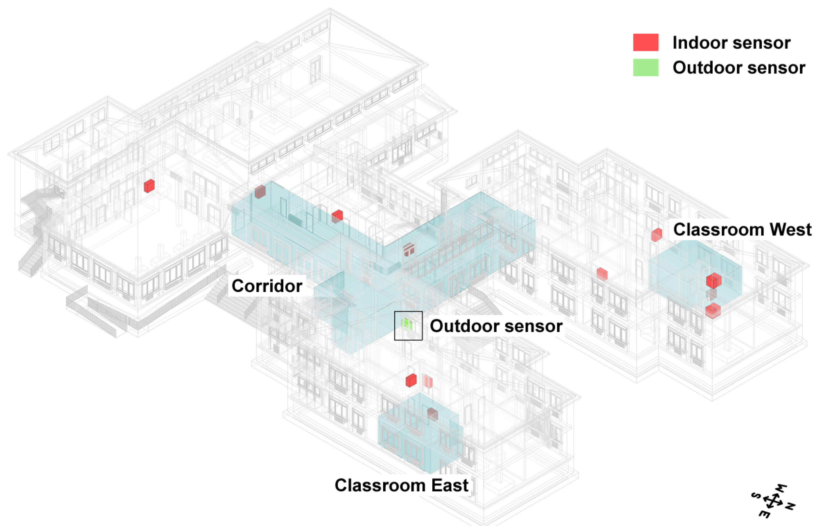
To obtain a suitable dataset for our study, we first analyzed the structural information of the building (i.e., geometry, materials, thermal and physical properties of building components) and then we built its BIM model, that is reported in Figure 1.

To provide a thorough analysis, we decided to focus our study on the building as a whole, as well as three representative rooms, chosen based on symmetrical shapes and regular internal distribution: (i) a classroom facing west, (ii) a classroom facing east and (iii) the corridor at the main entrance. Both classrooms are comparable in terms of size, internal characteristics, use and occupants and differ only in the orientation. Hence, they reasonably represent two opposed thermal conditions of the same type of classroom. The corridor is not characterized by a constant occupancy during working hours. Nonetheless, it is considered significant for this study because it is a very large environment located in a central position of the building, with many openings and glazed windows.

In the real-world building, we deployed 13 IoT devices to monitor the air-temperature trends (see Figure 1) with a sampling rate of 15 min. To do so, we used ST-Microelectronics STM32 Nucleo-64 boards [44] equipped with a low power transceiver module SPIRIT1 [45]. However, the collected dataset (7777 samples in total) is not large enough to train a prediction model. Thus, we generated an enlarged dataset by simulating the thermal energy behaviour of the building with EnergyPlus, exploiting our BIM model together with real weather data of about six years, from 2010 to 2015. Traditionally, EnergyPlus simulations take as input TMY data. As we demonstrated in our previous work [8], real weather information can provide indoor air-temperature trends (in the form of time series) with a lower error rate. Hence, we followed this approach in our study, obtaining a realistic dataset with values sampled every 15 min. In detail, we considered all the values between November and March that is the operational period of the building heating systems in our country. Then, we split the synthetic data into two independent subsets for training and testing purposes, containing about $70\%$ and $30\%$ of the initial samples, respectively. The training set (71,901 samples in total) was used to train the prediction models and optimize their parameters, whilst the test set (14,303 samples) was used to assess the prediction performance (see Section 5.1). The dataset with the real measurements (7777 samples at 15 min sampling rate) was also employed, but just for testing purposes (see Section 5.2).

4. Methodology

To predict the indoor air-temperature of a building in short- and medium-term, we need to work with time series information. For this purpose, methodologies based on Artificial Neural Networks are very promising [46]. An ANN is composed of units, called nodes or neurons, typically organized in one layer of inputs, one or more hidden layers and one output layer. The simplest topology of the network is the Multi-Layer Perceptron (MLP), that is feed-forward and fully connected. Connections are associated to adjustable parameters called weights that represent the strength of a connection between two nodes. Each neuron is a simple computational unit that applies a non-linear activation function to the sum of the weighted inputs.

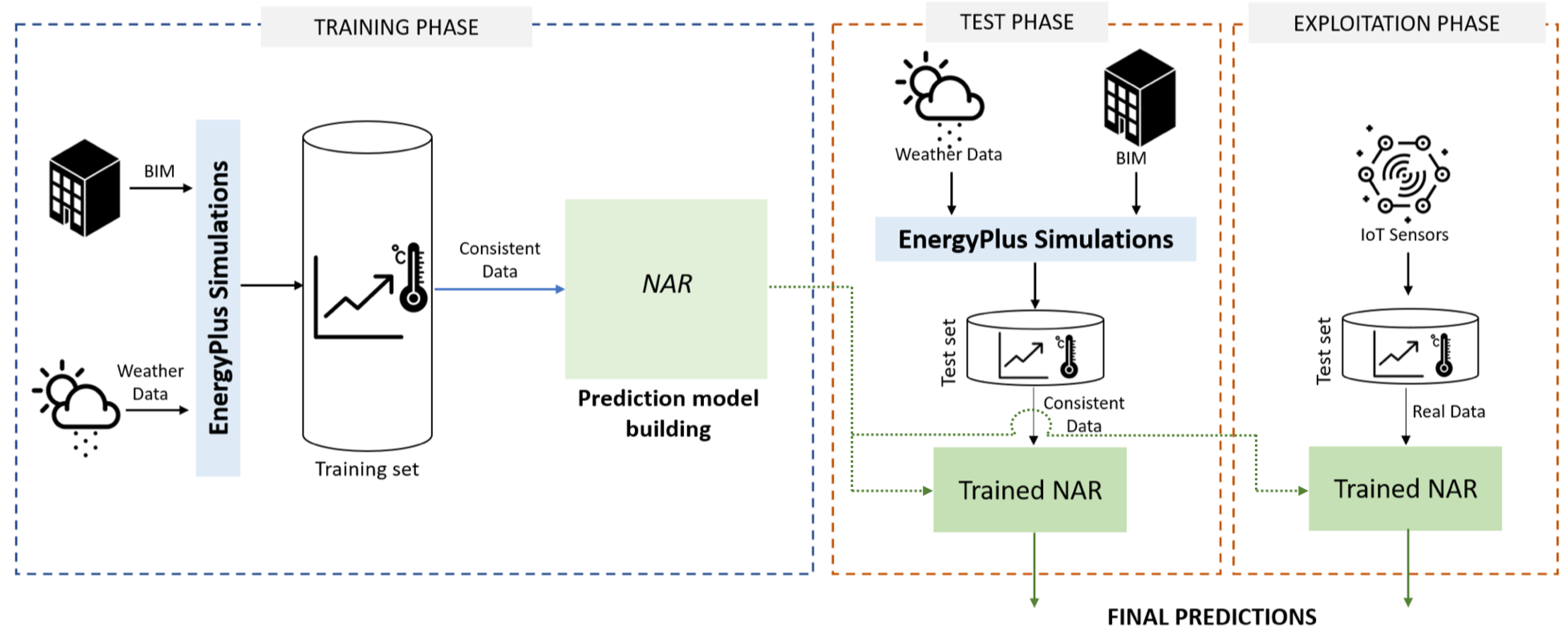
In this work, we designed a Nonlinear Autoregressive neural network and we optimized the model on four different environments chosen as case study, i.e., the three relevant rooms and the whole building (see Section 3). In Figure 2, we show the main steps of our proposed solution. During the training phase, time series data consisting in realistic artificial indoor-air temperature trends (see Section 3) are given as input to build a prediction model based on NAR. In the test phase, new unseen data from the realistic artificial test set are fed into the trained models to obtain the temperature predictions. Finally, in the exploitation phase, new unseen data sampled by IoT devices (deployed in the real-world building) are given as input to the trained models to evaluate the final predictions against real indoor air-temperature values. The rationale of splitting the experimental assessment into two different phases (test and exploitation) is the following. In the test phase, the model is tested on a large synthetic dataset obtained with EnergyPlus simulations, as for the training. Hence, the aim of this test is assessing the prediction capabilities of the model in a significant number of examples. In the exploitation phase, the NAR is assessed on a much smaller real-world dataset, which is less representative in terms of size but on the other hand provides better insights into the generalization capabilities of the model in real-life conditions. On top of that, it provides an indirect assessment of the reliability of the synthetic data that were used for training the model.

In the following, we report in details the main phases of the system, describing: (i) how we selected and identified the final architectures and related parameters of the prediction models and (ii) how we optimized such parameters to boost the performance and robustness of the models, preventing the risk of over-fitting.

Nonlinear Autoregressive Neural Network

NAR is an ANN that extends a traditional linear autoregressive model [47] to be completely distribution-free. Thus, NAR is suitable for non-linear time-series that report, for instance, unexpected spikes and fleeting transient periods [48].

A NAR model forecasts a value of a signal y at time t using n past values of the signal y as regressors, following the Equation (1):

$$y\left(t\right)=f\left(y\right(t-1),y(t-2),...,y(t-n\left)\right)+e\left(t\right),$$

(1)

where f is an unknown non-linear function and $e\left(t\right)$ is the model approximation error at the time t.

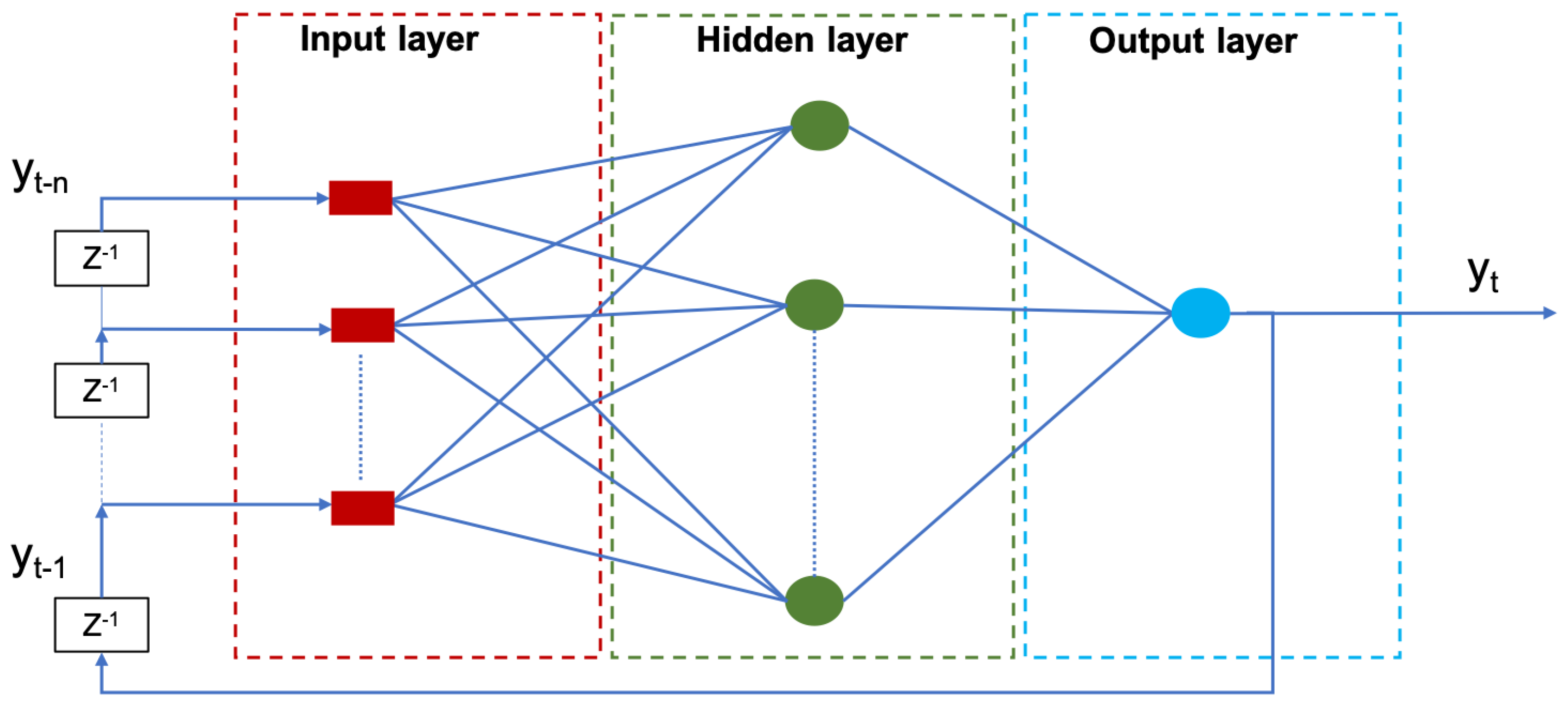
Function $f\left(·\right)$ is given by optimizing a multi-layered ANN, whose topology is represented in Figure 3.

At the time t, the ANN is fed with the n regressors of the signal y. These inputs are transferred through multiple layers of neurons. Each neuron is a computational unit characterized by (i) a set of weights W (one per each input connection j), (ii) a bias b and (iii) an activation function h. Hence, a neuron i computes its output following the Equation (2):

$$ou{t}_i=h_i\left(\sum _j{w}_{i,j}·i{n}_{i,j}+b_i\right)$$

(2)

where $w_{i,j}$ and $b_i$ are computed by back-propagation on the training set [48].

To design the NAR model, the starting point is the selection of the lag-space, that in our application is the optimal number of past air-temperature values to be used as regressors. For this purpose, we applied Lipschitz methodology [49], that is a well-known approach in the analysis of input-output models’ orders in nonlinear dynamic systems that allows to empirically determine the number of regressors of a system. By applying this method as described in [50], we found $n=13$ as the best candidate. This value is not the final optimum of our system, but a reference point for a more in-depth empirical analysis. Thus, we implemented a grid search to find the optimal value, testing the performance of different ANNs varying the number of regressors within a 20-dimensional range of values centred in $n=13$. This approach was implemented for each selected room and for the whole building, respectively. In each configuration, we started with fully-connected NAR ANNs as shown in Figure 3, with the following characteristics:

• one input layer with a variable number of regressors decided by our grid search;
• one hidden layer with 30 neurons;
• one output layer with one neuron.

This architecture is the result of our preliminary experiments with different network structures, where we found that increasing the number of hidden layers (and hence the complexity and computational costs of the training) did not provide significant benefits in terms of prediction performance. For all the configurations, we used hyperbolic tangent activation functions for the hidden neurons and a linear activation function for the output neuron, as shown in Figure 4.

Then, we chose and implemented the Levenberg-Marquardt back-propagation procedure (LMBP), which is a learning paradigm widely applied to NAR ANNs in literature [51]. LMBP reduces the training speed compared to other back-propagation techniques because it approximates second-order derivatives leveraging a trust region approach [48] without computing the Hessian matrix. These models were trained on the training set described in Section 3. We found that the best training performance was obtained with 20, 19, 16 and 20 regressors for respectively the classroom facing East, the classroom facing West, the corridor and the whole building (see Section 3). The second column of

Table 1. Validation error (nSSE) before and after OBS pruning.

NAR Network Type	nSSE before Pruning	nSSE after Pruning
Classroom facing East (20 regressors)	9.95 × 10−3	9.51 × 10−3
Classroom facing West (19 regressors)	1.59 × 10−2	1.54 × 10−2
Corridor (16 regressors)	1.87 × 10−2	1.85 × 10−2
Whole building (20 regressors)	1.19 × 10−2	1.17 × 10−2

reports the normalized sum of squared errors (nSSE) on the validation set obtained after the training phase for all the different networks.

As it is widely known, ANNs with too many connections have longer training procedure and may easily lead to over-fitting. To overcome this issue, we pruned the initial fully-connected structures adopting the Optimal Brain Surgeon (OBS) methodology [52]. The rationale of this operation is to remove redundant connections between neurons to obtain more efficient and compact models than the initial ones, not affecting or possibly improving their prediction capability. OBS estimates the increase in the training error when deleting weights, leveraging information in the second-order derivatives of the error surface. This procedure works towards the minimization of the error variation, computing recursively the inverse Hessian matrix from the training data to achieve better approximations of the error function (more details are provided in [52]). Dong et al. [53] demonstrated that OBS performs better than other pruning techniques by removing more redundant neuron connections.

After pruning, the four different ANNs were trained again with LMBP. The new nSSE values provided by this second round of training are reported in the third column of Table 1. The values if this table highlight that OBS pruning was successful, as it further reduced the validation error of the four NAR models.

5. Experimental Results

The purpose of our methodology is to make predictions of indoor air temperature values in buildings in order to enable new energy policies. To achieve this target, the predictions need to be as accurate as possible while providing the longest time horizon possible. To assess the ability of our system to achieve this goal, we split the experimental assessment into two different phases, as shown in Figure 2: (i) test, where the model was tested on a large set of simulated data in order to obtain a reliable estimate of the prediction accuracy and prediction window; (ii) exploitation, where the same model trained on synthetic data was tested on a smaller dataset of real measured data. This second assessment provides information about the robustness of the model in real-life conditions, as well as on the reliability of the simulations that were used for the training. For the two phases, we used the datasets described in Section 3 that are both completely independent from the one used to train and optimize the model.

In both cases, the goodness of the predictions was first established by measuring the similarity between the predicted and the observed values, used as the ground truth. For this purpose, we adopted metrics that are widely used in statistical analysis and more specifically in time-series analysis literature [54]:

• Mean Absolute Difference (MAD), defined as the average absolute difference between predicted and observed values;
• Root Mean Square Difference (RMSD), defined as the standard deviation of differences between predicted and observed values.

5.1. Test on Simulated Data

In our first set of experiments, the model trained on simulated data was tested on an independent dataset, even in this case obtained by simulations. As already discussed in Section 3, our overall simulations included 6-year indoor air-temperature values at 15 min intervals, obtained with the strategy presented in [8]. As the test-case building contains a total number of 115 rooms, including uninhabited areas such as basements and attic, we decided to focus our study on three most representative rooms (facing East, facing West and Corridor) as well as on the building as a whole, obtained as the average of all the 115 time-series. This implies that the four NAR models described in Section 4 were trained on a training set containing the temperature time-series corresponding to the four different environments and then tested on the corresponding test sets. We made experiments at different prediction windows, up to a maximum of 270 min.

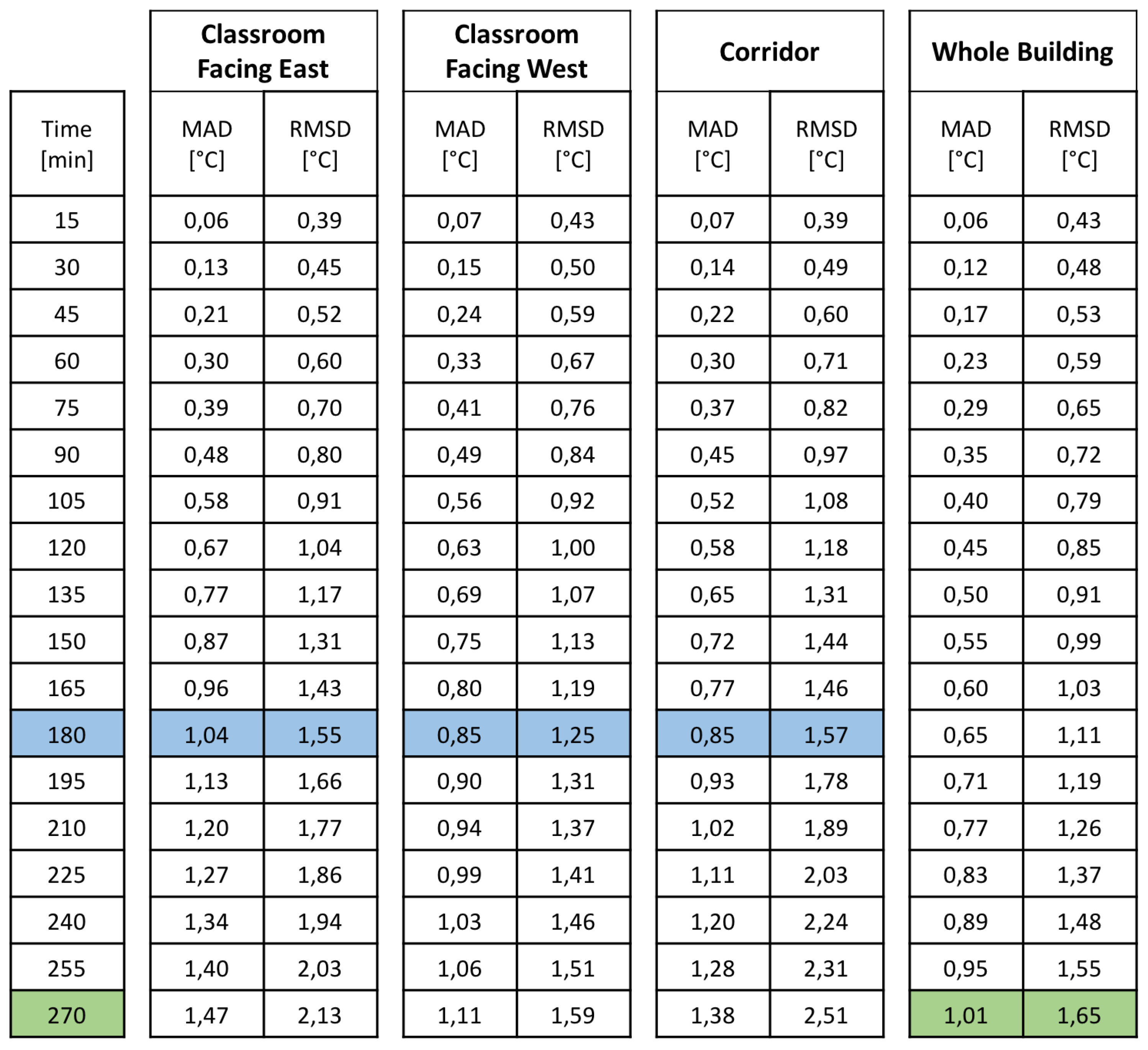
In Figure 5 we report the values of MAD and RMSD obtained at different prediction windows (see first column of the Figure), separately for the three rooms of interest and for the whole building. As the building of our case-study is a public school, we focused our analysis on the only working hours.

By analyzing the values reported in the Figure, we can make the following considerations.

• As expected, the prediction performance worsens as the prediction horizon increases with more or less the same trend for the four different scenarios.
• The prediction accuracy is comparable for the three individual rooms with MAD and RMSD values differing by few fractions of degree at best, which is a variation that would be hardly perceived by the human occupants. This is quite remarkable, if we consider that the three rooms are very different from each other in terms of thermal conditions.
• When considering the whole building, the prediction accuracy is better than the one achieved on the three individual rooms. This can be easily explained if we consider that the temperature values of the building were obtained by averaging the temperatures of all the 115 rooms. The averaging smoothes off temperature spikes that might be present in the individual rooms, especially if these rooms are at the extremes of the temperature distributions of the whole building, like the three ones that were analyzed in our study.

According to most standards and literature studies, to guarantee no impact on the thermal comfort perceived by the occupants, the operative temperatures should never fluctuate more than $1.1{}^{\circ }$C ($2.0{}^{\circ }$F) within 15 min, nor change more than $2.2{}^{\circ }$C ($4.0{}^{\circ }$F) within 1 h [55,56]. Upon these considerations, in our study we established a value of MAD of about $1{}^{\circ }$C as the maximum acceptable threshold for our temperature predictions. Based on this conservative threshold, we assessed the maximum prediction horizons that can be guaranteed by our models. As it can be seen in Figure 5, this prediction horizon is 180 min when considering the individual rooms (see blue-coloured line) and 270 min for the whole building (see green-coloured line), which is quite a remarkable time-window. Compared to our previous work [7], we were able to improve MAD and RMSD performance index on average by $21\%$ and $13\%$, respectively.

5.2. Exploitation on Real Data

In our second set of experiments, the models trained on the simulated data were exploited on a small dataset of real temperature measurements that was described in Section 3. This dataset was sampled by temperature sensors operating in a range between $-40{}^{\circ }$C and $+120{}^{\circ }$C with a temperature sensitivity and accuracy of $0.016{}^{\circ }$C and $\pm 0.5{}^{\circ }$C respectively. The sampling frequency is 15 min and there are no missing values. Even though this second dataset is very limited in terms of number of data samples, and hence less significant for the performance evaluation, it can still provide very meaningful insights into the robustness of the predictions in real-life conditions, as well as into the reliability of the simulations that were used to generate the training data. The overall results obtained on the real dataset are shown in Figure 6 with the same content and format of the ones obtained on the simulated data.

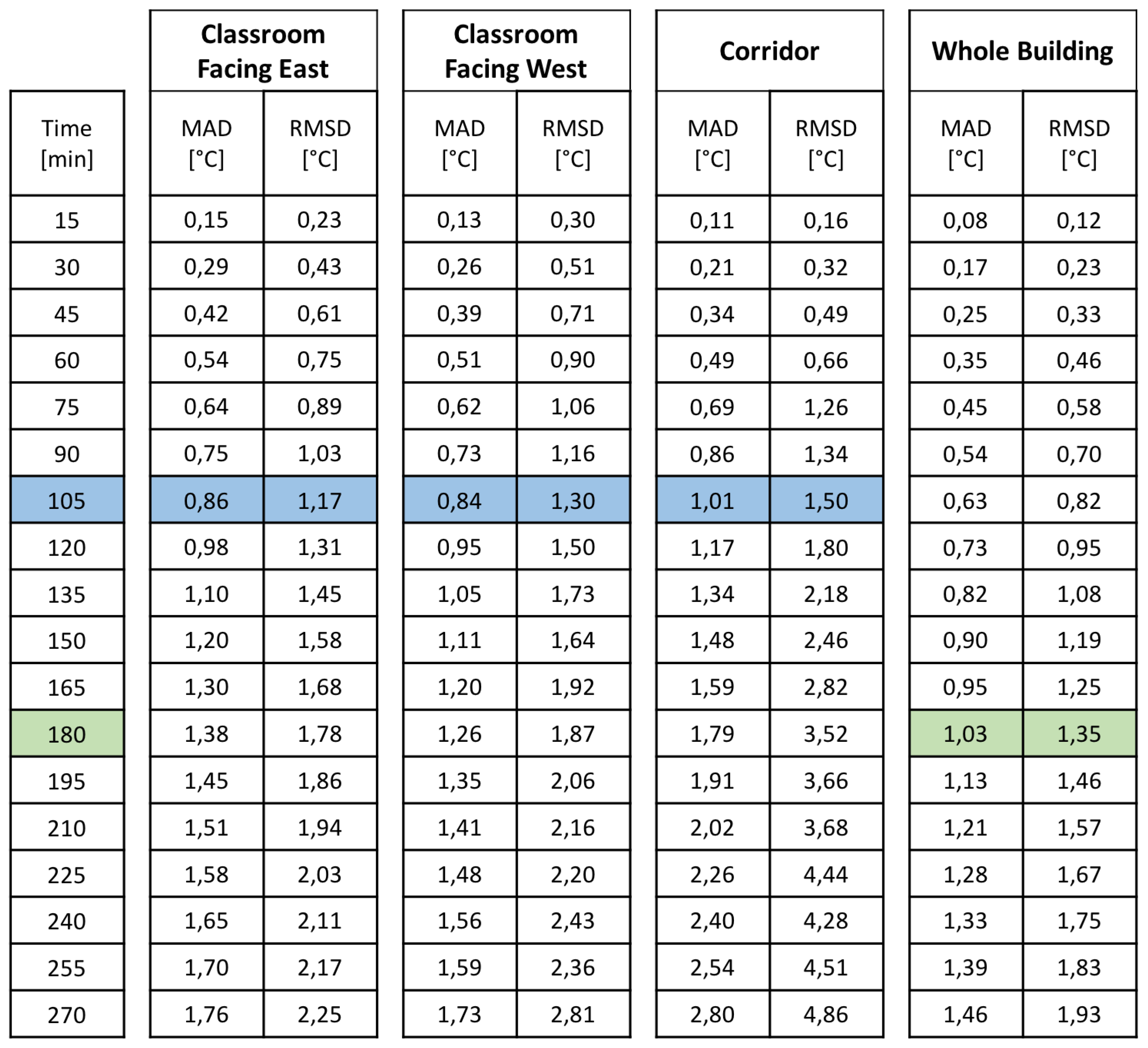
The prediction performance obtained on the real dataset is lower than the one obtained on the simulated dataset. This is reasonably due to some intrinsic differences between the real measurements data and the simulated ones. For example, due to some unpredictable actions of the human occupants (e.g., opening/closing windows), which might considerably change some temperature values.

If we establish again a value of about 1 ${}^{\circ }$C as the maximum acceptable threshold on MAD, we obtain that the maximum prediction horizons of our models on the real data are 105 and 180 min, respectively for the individual rooms (blue line in Figure 6) and the whole building (green line in Figure 6). While these horizons are lower than the ones estimated on the simulated data, they are still remarkably long, which confirms the wide usability of the model in Demand Response applications [10,11,12].

All the other considerations made on the simulated dataset are still valid.

Besides the traditional assessment based on prediction performance, the goodness of a temperature prediction model can be evaluated indirectly by estimating the impact that a temperature change w.r.t. the observed values would eventually have on the well-being of the occupants. To do so, in our work we exploited the method described in [55], which is implemented in most international standards for the design, operation, and commissioning of occupied spaces [56,57], on our real measurements dataset.

This method leverages upon the quantification of the following two metrics:

• Predicted Mean Vote (PMV), a −3 to +3 index estimating the state of well-being of a group of individuals, where −3 means feeling too cold, +3 means feeling too hot and 0 represents a perfect thermal well-being.
• Percentage of Person Dissatisfied (PPD), a 0 to 100 value estimating a percentage of people dissatisfied by the thermal conditions of the environment.

More specifically, in our analysis we exploited the well-known sensation scale defined in [55], which puts in relation the values of PMV and PPD and defines the thermal comfort area as the range of values for which $-0.5<PMV<+0.5$. As reported by [55], this range is associated to the maximum probability of having at least 90% of the population of occupants completely satisfied by the thermal conditions of the environment.

More specifically, we applied the following procedure:

• We computed PMV/PMD indices for all the target environments of our real-world demonstrator. Again, we focused only on the working hours, which are the ones that are significant for the temperature predictions.
• For each prediction horizon, we computed the percentage of predicted values that are within the $\pm 0.5$ PMV thermal comfort area.

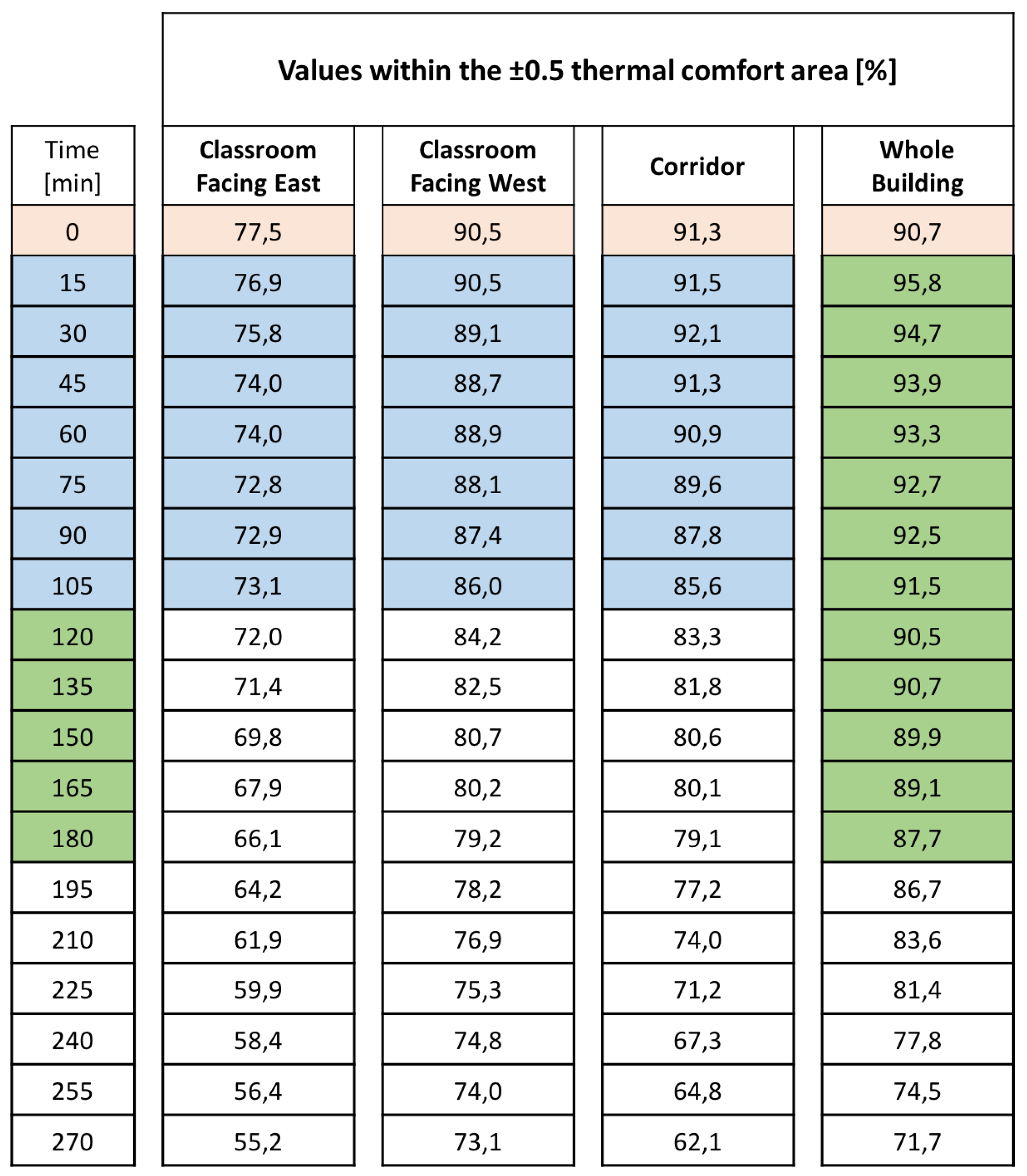
The obtained results are reported in Figure 7, separately for the three individual rooms and the whole building models. The first row of the table in Figure (at time 0, red coloured) shows the thermal comfort values obtained on the observed data, which can be used as a reference. The following rows of the table in Figure report the thermal comfort values obtained on the predicted data at increasing prediction horizons. The rationale of the experiment is: the closer the thermal comfort values to the corresponding reference values at time 0, the better the prediction. The blue and green areas in the Figure correspond to the prediction windows that were identified as reliable in our previous prediction performance analysis on the same data (respectively up to 105 min for the individual rooms and 180 min for the whole building).

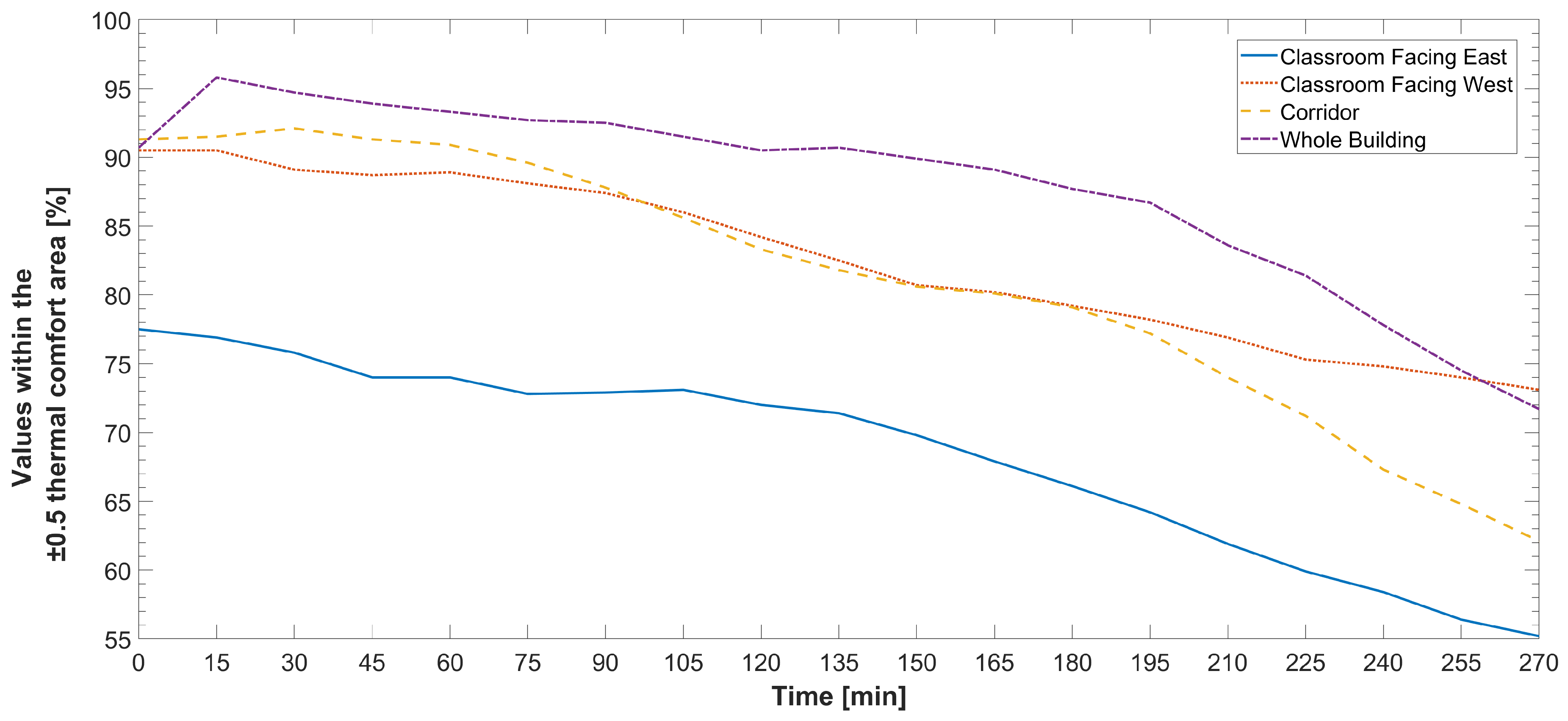
If we look at the blue and green areas, we can observe that the values are generally high, with a difference with respect to the reference values that is always below 6% for the individual rooms and below 3% for the whole building. As for the prediction performance metrics, the percentage of predicted values within the thermal comfort zone tends to decrease with the prediction horizon, even though with some minor oscillations. Figure 8 clearly shows this trend.

Nonetheless, the values do not have a sudden drop even outside the nominal prediction windows of 105 and 180 min, which confirms that our thresholds were conservative enough. Again, the performance of the models in different types of environments are comparable.

6. Conclusions and Future Works

In this paper, we proposed a novel methodology to forecast indoor air-temperature in Smart Buildings exploiting realistic synthetic data to train prediction models based on a NAR architecture with a high number of regressors. We also discussed the prediction accuracy of our models by analyzing the inference results both on synthetic and real data. The aim of our methodology is trying to compensate for the lack of real-world data in the context of energy simulations for the energy-efficient management of Smart Buildings. As a matter of fact, buildings are very rarely equipped with suitable temperature sensors and, even in the case the sensors are available, the amount and significance of historical data might not be enough to train a prediction model. In our methodology, BIM and meteorological data are exploited to construct of a realistic and consistent dataset of temperature values. This dataset can be used to train NAR networks that are specifically designed to provide realistic temperature predictions of a specific type of room or of building. As demonstrated by our case study, our models provide accurate predictions with time horizons in the order of 3 h for individual rooms and 4 h for the entire building.

The predictions provided by our models can be exploited for the design of control policies for the energy-efficient management of Smart Buildings (e.g., Demand Response, Demand Side Management and peak-shaving, which are all based on thermal behaviours forecasting), especially for those scenarios where real sensors data are unavailable or insufficient.

In our future work, we will extend our indoor air-temperature forecasting system by integrating real-time information. More specifically, we plan to introduce the possibility of a real-time fine-tuning of our prediction model, leveraging the indoor air-temperature measurements eventually provided by IoT sensors equipped in the Smart Building. In addition, we plan to further improve the proposed methodology addressing possible noise or missing data scenarios during the inference phase [58].