Dynamic Deep Forest: An Ensemble Classification Method for Network Intrusion Detection

Abstract

Network Intrusion Detection System (NIDS) is one of the key technologies to prevent network attacks and data leakage. In combination with machine learning, intrusion detection has achieved great progress in recent years. However, due to the diversity of intrusion types, the representation learning ability of the existing models is still deficient, which limits the further improvement of the detection performance. Meanwhile, with the increasing of model complexity, the training time becomes longer and longer. In this paper, we propose a Dynamic Deep Forest method for network intrusion detection. It uses cascade tree structure to strengthen the representation learning ability. At the same time, the training process is accelerated due to small-scale parameter fitting and dynamic level-growing strategy. The proposed Dynamic Deep Forest is a tree-based ensemble approach and consists of two parts. The first part, Multi-Grained Traversing, uses selectors to pick up features as complete as possible. The selectors are constructed dynamically so that the training process will stop as soon as the optimal feature combination is found. The second part, Cascade Forest, introduces level-by-level tree structures. It has fewer hyper-parameters and follows a dynamic level-growing strategy to reduce model complexity. In experiments, we evaluate our model on network intrusion dataset KDD’99. The results show that the Dynamic Deep Forest method obtains higher recall and precision through a short time of model training. Moreover, the Dynamic Deep Forest method has lower risk of misclassification, which is more stable and reliable in a real network environment.

1. Introduction

The rapid development of Internet facilities people’s daily lives, but also brings potential risks. A survey released in 2017 provides a comprehensive summary of intrusion in networks [1]. It states that security is a major concern among all types of information flow between the end devices. Various network intrusions will lead to disturbing problems, such as congestion, performance degradation, and even network collapse, causing unnecessary property loss. Therefore, it is of great significance to detect network intrusion in time. In this way, measures can be taken to ensure network security.

Network Intrusion Detection System (NIDS) is considered as a key part to detect anomalies and network attacks. The NIDS can be categorized as Misuse Detection (MD) and Anomaly Detection (AD) [2]. MD uses patterns or signatures based on existing attacks to detect known intrusions. It defines the behavior of abnormality and performs a pattern matching for the network attacks. Although MD can add common attack types to the model easily, it is not good at dealing with new and unknown attack types. From another perspective, AD can explore regular features from normal traffic, and then discover unknown attack behaviors in a short time. Compared to MD, AD is a more important detection method in the practical use.

In recent years, machine learning (ML) technology has been introduced in NIDS, which has advantages in feature extraction and improves the classification accuracy among different attack types. For example, Sahil Garg et al. [3] proposed an ensemble-based classification model for network intrusion detection. They used Hoeffding-bound based clustering to identify the feature subsets and reached a high level of accuracy. From another point of view, Nathan Shone et al. [4] used deep autoencoder, a deep learning approach to solve the same problem. The experiments proved that they also obtained competitive results.

As a matter of fact, it is not enough to only consider the detection accuracy when evaluating the model performance. In a real network environment, the percentage of intrusion is small. So the classification accuracy can always be maintained at a high level. Besides, unknown attack behaviors evolve quickly, which places high demands on the model generalization ability and training speed. Deep learning methods have been popular in recent years. They consist of layer-by-layer neural networks and have strong representation learning ability. However, due to the large number of parameters in deep learning methods, much time will be invested in the training process. In order to improve the model practicability, we are committed to building a model that not only retains the feature representation ability like deep learning, but also considers other evaluation indexes, such as recall, model training time, and so on.

In this paper, we propose the Dynamic Deep Forest, an ensemble method for network intrusion detection. The Dynamic Deep Forest consists of two parts. The first part Multi-Grained Traversing uses selectors to pick up features as complete as possible. The selectors are constructed dynamically so that the training process will stop as soon as the optimal feature combination is found. The second part Cascade Forest introduces level-by-level tree structures. Each level of cascade receives feature information processed by its preceding level, and outputs its processing result to the next level. Besides, cascade forest follows a dynamic level-growing strategy: the growth of decision tree levels will stop if there is no significant performance gain by expanding a new level. In summary, dynamic deep forest constitutes three advantages in the following aspects: (1) A dynamic selector to combine network features and strengthen representation learning ability. (2) A dynamic tree level-growing strategy to reduce model complexity and speed up model training. (3) A tree-based model structure to avoid large-scale parameter fitting and suitable for NIDS classification problems.

2. Related Works

This section is divided into two parts. In the first part, we will discuss some mainstream machine learning methods applied to NIDS. In the second part, the idea of the Dynamic Deep Forest will be introduced.

2.1. Mainstream Methods in NIDS

There are mainly two kinds of solutions to detect intrusion:the first is traditional machine learning methods and the second is deep learning. Both of the solutions can get a high level of detection accuracy.

In traditional machine learning fields, ensemble methods are the most popular due to their high classification performance and fast training speed. Researchers combine various weak classifiers together to construct a new and strong classifier. By doing this, their models become more powerful to decrease bias and variance.

In the initial stage of using ensemble in NIDS, a clustering algorithm and some basic filters are given preference. For example, Garg et al. [5] used a combination of fuzzy K-means clustering algorithm and extended Kalman filter to detect the intrusion. Experimental results indicated that the proposed ensemble technique achieved high detection accuracy with low false positive rate (FPR) as compared to its traditional counterparts.

As time going by, support vector machine (SVM) is gradually considered as a good classifier in ensemble, along with some dimension reduction methods. For example, Aburomman et al. [6] used an ensemble of Linear Discriminant Analysis (LDA) and Principle Component Analysis (PCA) to maximize the effectiveness of the feature extraction algorithm. In the training stage, ten binary SVM classifiers were combined with Weighted Majority Voting (WMV) so that every classifier becomes an expert in that region space. This ensemble PCA-LDA method has good results with a fast model training speed.

With the development of machine learning, an increasing number of options are made available to researchers. Wang et.al. [7] put forward an ensemble learning method, which employed bayesian network and random tree as basic classifiers. The model combined the advantages of both bayesian network and random tree, making it suitable for various scales of sample classes. Besides, it speeded up the feature selection process and had a better effect on sensitivity and specificity.

In deep learning fields, by means of the strong representation learning ability, there are also several methods within the domain of NIDS, such as deep neural network, extreme learning machine, and autoencoder.

Deep Neural Network (DNN) is a flexible and powerful model in deep learning. Kim et.al. [8] designed a DNN with four hidden layers and 100 hidden units to target advanced persistent threats. Rectified Linear Unit activation (RELU) was adopted as the activate function, which can express a complicated classification boundary and enhance the model performance. The results showed a significantly high accuracy.

To handle concept drift problems in a continuous data stream, Xu et.al. [9] proposed a dynamic extreme learning machine (DELM) for classification of patterns. The algorithm used ELM as the base classifier and set a threshold to detect concept drift. When an intrusion alert was sent, more hidden layer nodes were added to the neural network to improve the performance of the classifier.

Apart from DNN and DELM, Javaid et.al. [10] proposed another deep method to build an effective NIDS. Their method was called self-taught learning (STL), which combined a sparse auto-encoder with softmax regression. They implemented their solution and evaluated it against the benchmark NSL-KDD dataset. The authors claimed some promising levels of classification accuracy in both binary and 5-class classification.

In conclusion, ensemble methods can obtain a competitive performance through a short time of model training. On the other hand, deep learning achieves a great performance due to the powerful representation learning ability. Therefore, we are aimed to make a combination of ensemble methods and deep learning. In this way, we can improve the detection performance while speeding up the training process.

2.2. The Idea of Dynamic Deep Forest

In real network environment, data stream is dynamic, ever-changing, and requires rapid response [9]. To ensure the accuracy of intrusion detection, the model should be updated in time, which places demands on model training speed. We try to build a deep model in tree-based structure, which can not only avoid large-scale parameter fitting to save time, but also keep representation learning ability, like deep learning.

Tree-based methods gained extensive attention after the concept of bagging was introduced in 1996 [11]. Bagging is one of the ensemble techniques, which utilizes a bootstrapping algorithm to do sampling with replacement [12]. In this way, the variance of the model will be decreased. Actually, researches from Kontschieder [13] proved that a combination of bagging techniques and Deep Neural Network (DNN) performs better than just using DNN. On the other hand, Cheng Guo [14] elucidated that DNN cannot reach its fullest potential when faced with data mining problems sorted by structured data. This study makes us realize that in network intrusion problems, deep learning is not the best choice since the data is structured. In conclusion, our purpose of using ensemble is to get rid of DNN but still reserve the representation learning ability.

Boosting is another popular ensemble method [15]. It consists of iteratively learning weak classifiers with respect to a distribution and adding them to a final strong classifier. Boosting is the inspiration of the cascade procedure [16], which is able to automatically decide the number of learners in an ensemble. We build the model based on the structure of cascade boosting, which is effective and had been proved useful by many people [17]. Besides, Zhou [18] published their work in 2012, emphasizing that diversity is crucial for ensemble construction. Therefore, our model adds various tree-based classifiers to encourage the diversity.

Inspired by the idea above, the Dynamic Deep Forest was eventually proposed and divided into two parts. The first part is Multi-Grained Traversing. It is the step which uses selectors to pick up features as complete as possible. The larger the size of a selector is, the more features a sample will possess. At the beginning of the model training, a small size of the selector will be used to choose features and combines them as a sample. Then the processed samples will be input to train both a Random Forest model and an Extra-Tree model. In addition, the number of the selectors is dynamically determined. Unless the loss function in Multi-Grained Traversing stopped decreasing, a bigger size selector will be introduced, which combines more features together. This is actually different from Multi-Grained Scanning in gcForest [19], which uses sliding windows to examine the image data.

Multi-Grained Scanning is good at extracting spatial relationships among the raw pixels, so it has advantages when data is in image format. But in real network intrusion problems, data is usually structured. The relationship between different features is not as obvious as adjacent pixels in image. Therefore, it’s necessary to explore all the possibilities of feature combination rather than just sliding windows in structured data training. Based on the above analysis, we propose Multi-Grained Traversing to combine different features together decided by the size of the selector. And in this way, multiple instances could be produced to describe feature relationships and strengthen representation learning. Figure 1 intuitively illustrates the distinction between Multi-Grained Scanning and Multi-Grained Traversing.

The second part is Cascade Forest. It is actually a cascade tree structure, including LightGBM [20] and XGBoost [21] as the basic model in each level in order to encourage the diversity. Compared to gcForest, the Dynamic Deep Forest shows differences in three points: (1) Using Multi-Grained Traversing rather than Multi-Grained Scanning for network traffic data training. (2) Adding a dynamic selector to combine initial features and strengthen representation learning ability. (3) Composing ensemble construction of LightGBM and XGBoost for better representation learning.

3. Details of Dynamic Deep Forest

In this section, we will introduce the two partitions of dynamic deep forest, respectively. The implementation of multi-grained traversing and the cascade forest will be given in detail. Followed by the overall architecture presented with specific parameters.

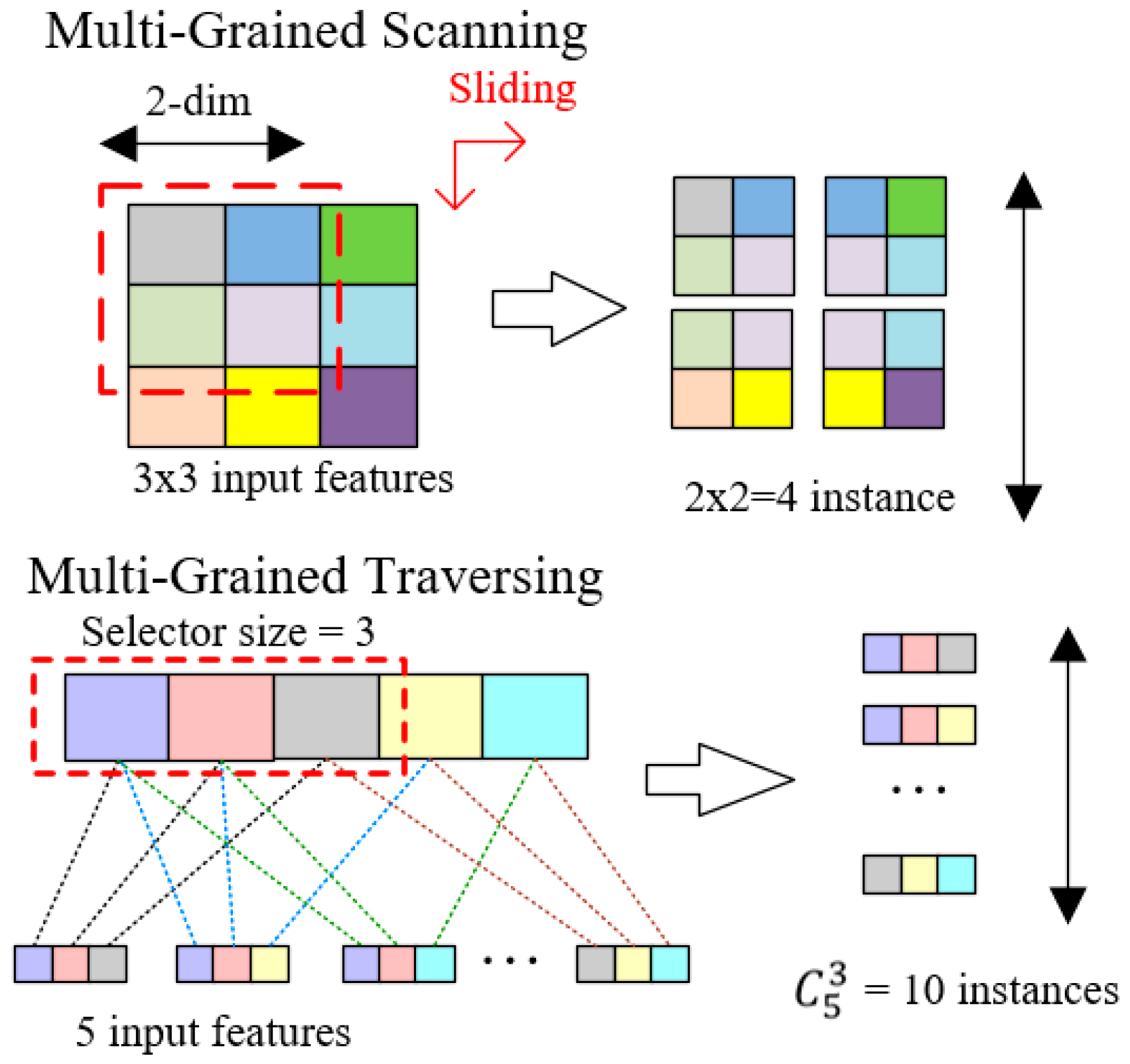
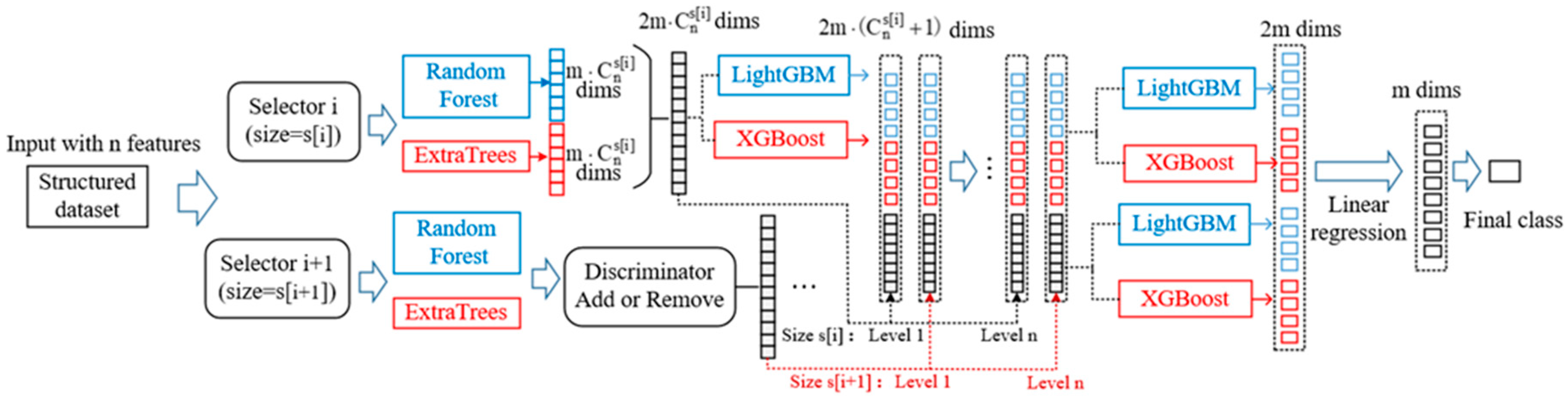
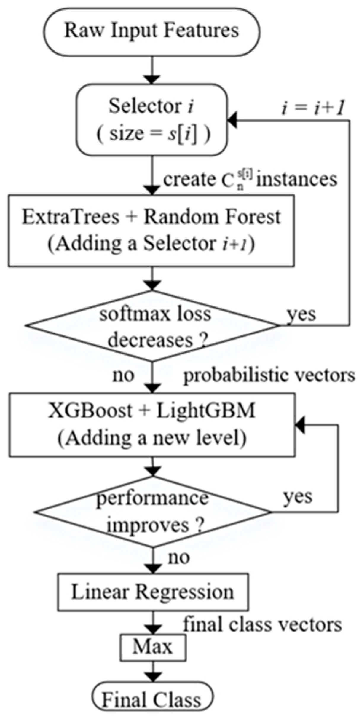
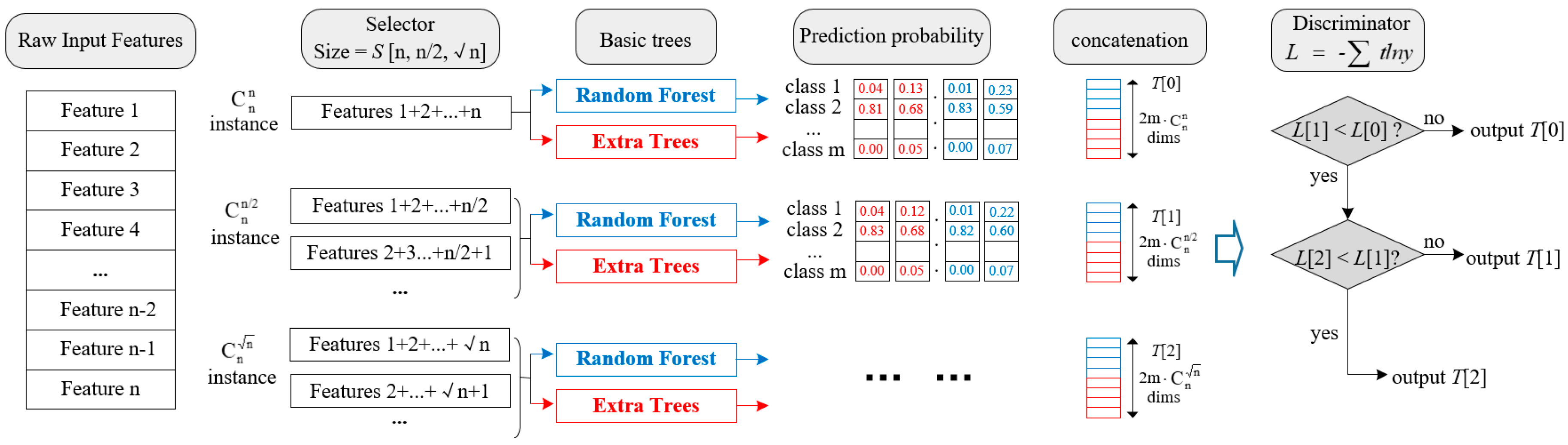
3.1. Dynamic Multi-Grained Traversing

Multi-grained traversing is the process to do feature combination by different sizes of selectors. This is a pre-processing procedure to strengthen the representation learning ability. A dynamic set of selectors is the main bright spot in this part, which considers both the loss function and training time. In network intrusion multi-classification problems, cross-entropy loss is used as the loss function, and the specific formula is shown below:

$$Loss=-{\displaystyle \sum }_i{t}_{i}ln{y}_i$$

(1)

where $t_i$ means the ground truth of ith sample. $y_i$ is the prediction, which is the output of softmax activation function:

$$y_i=\frac{e^{x_i}}{{\sum }_k{e}^{x_k}}.$$

(2)

where $x_i$ means the feature vectors of i th sample.

There are 3 different sizes of selectors in a dynamic selector set. Suppose there are n features in a sample and m classes need to be classified. The sizes of selector sets can be expressed as $S=\left[n,n/2,\sqrt{n}\right]$. The setting of selector size refers to random forest [22], which is composed of several weak decision trees. Each decision tree contains a part of feature set. And the max feature number is limited to $\sqrt{\mathit{n}}$. We are inspired by such feature selection methods and choose $\sqrt{\mathit{n}}$ and $\mathit{n}/\mathbf{2}$ as the selector sizes. In this way, model diversity can be increased as well as reducing the variance.

First, we choose the size of S[0] = n. It means all of the n features will be used to construct instances. Using the formula of combination, we can get $C_n^n$ = 1 instance. Under this circumstance, we do not do feature selection, and just input the raw samples to train both a Random Forest model (RF) and an ExtraTree model (ET). Two class vectors with m dims will be generated from the two tree-based models. By concatenating all the class vectors together, a long vector containing probabilistic information is finally transformed. The long feature sequence will not only be considered as the input of cascade forest, but also the prediction of Multi-Grained Traversing to calculate the cross-entropy loss L[0]. Afterwards, we will add the size of S[1] = n/2 and get $C_n^{n/2}$ instances. Combining with the size of S[0], we will have $C_n^n+C_n^{n/2}$ instances in total. Repeating the operation above, a new cross-entropy loss L[1] will be obtained. If L[1] < L[0], the value of loss function decreases and S[1] should be kept. Otherwise, we will keep S[0] only to save training time. To sum up, the growth of selectors will stopped if there is no significant perfofmance gain. And the algorithm for the selectors adding strategy is demonstrated in Algorithm 1.

Algorithm 1:Selectors Adding Strategy

Input: Raw Input Features

Output: Final probabilistic vectors, number of selectors

1:  procedure FUNCTION(Strategy)

2:   Initialize $S=\left[n,n/2,\sqrt{n}\right]$, i = 0.

3:   for each size of selectors in S do

4:    In selector i, size = S[i], create $C_n^{s\left[i\right]}$ instances.

5:    Concatenate all the instances produced before, the total number of instances is ${\sum }_0^i{C}_n^{s\left[i\right]}$.

6:    Compute probabilistic vector T[i] using library function of RF and ET in scikit-learn.

7:    Compute Loss L[i] using Equation (1)

8:    if (i = 0 || L[i] < L[i − 1]) continue

9:    else i = i − 1, break

10:   end if

11:   i = i +1

12:  end for

13: return T[i], i + 1

14: end procedure.

Besides, we choose Random Forest and Extra-Trees as the basic classifiers in Multi-Grained Traversing. Random Forest can sample features with replacement to construct leaf nodes, which decreases the variance of the model. Extra-Trees is an extremely randomized random forest. The bifurcation values are completely randomized instead of selecting the features with the best bifurcation properties.

The purpose of introducing these two models is to increase model diversity and randomness. Figure 2 illustrates the dynamic implementation of multi-grained traversing.

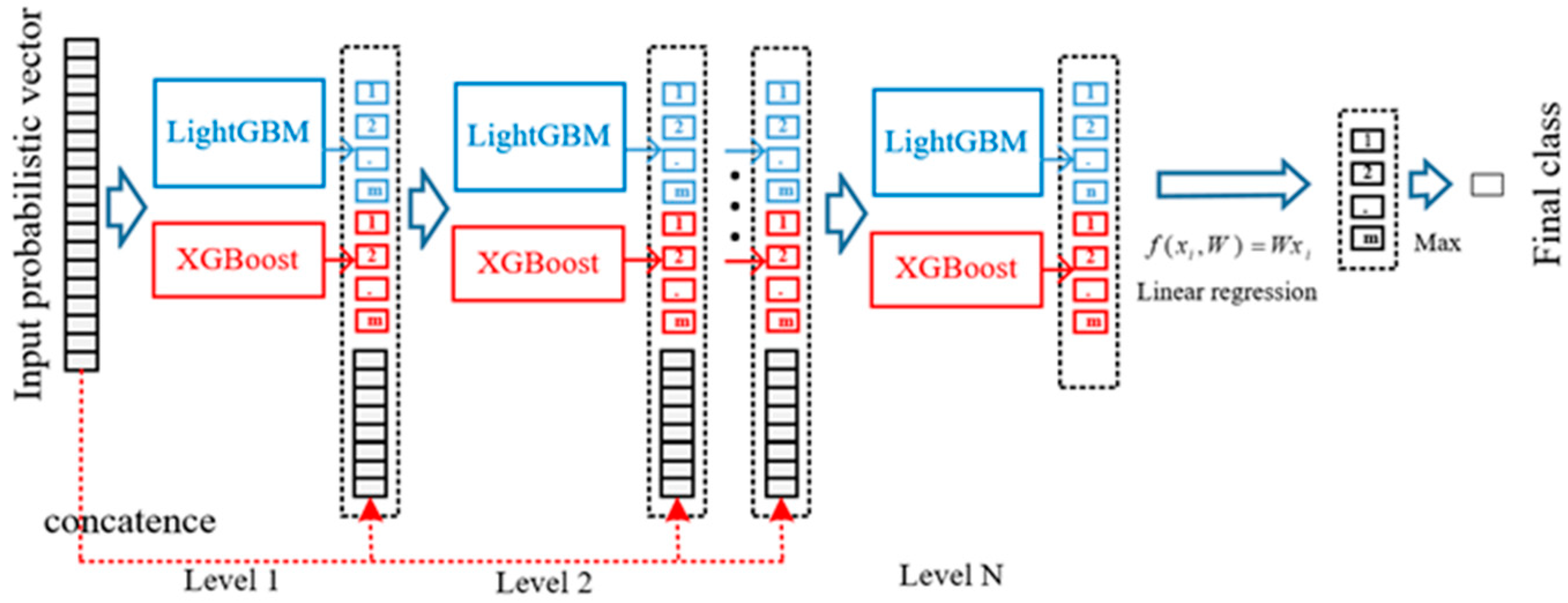
3.2. The Cascade Forest

In recent years, the number of layers in deep neural networks become deeper and deeper. Although these deep models obtained stronger representation learning ability and high accuracy, they costed more time in model training due to the large scale of parameters. Therefore, we try to find an alternative, which can not only get rid of the structure of deep neural networks, but can still retain the representation learning ability. Inspired by this magical layer-by-layer structure in deep models, we used a cascade form of tree structure as shown in Figure 3. After receiving the probabilistic vectors passed from the Multi-Grained Traversing part, the processed feature instances will be sent to train XGBoost and LightGBM in each level. In every level of cascade forest, the input will be the concatenation of probabilistic information processed by its forward level and the initial input probabilistic vectors at the beginning, the processing results will be sent to the next level.

In the same way, the number of cascaded levels is dynamically determined to reduce model complexity. If adding a new level can not improve the performance on validation set, then the growth of cascade levels will be removed. This operation takes an overall consideration on both the improvement of classification accuracy and the reduction of training time. It is worth saying that the dynamic selectors adding strategy and the dynamic level-growing strategy make it appropriate for various scales of data training. For a small-scale dataset, representation learning ability will be strengthened by the complete combination of features. And for a large-scale dataset, the number of selectors and cascade levels will be limited to speed up model training process.

Different from Multi-Grained Traversing, XGBoost and LightGBM were adopted as the basic classifiers in each cascade level. In the process of model training, a histogram algorithm used to improve training speed and efficiency, as well as reducing memory usage. In addition, sampling is performed using GOSS, which ensures that different sampling measures are taken depending on the data gradient.

The overall structure of Dynamic Deep Forest is shown in Figure 4. The number of selectors will be firstly determined according to the value of cross-entropy loss. Then, the probabilistic vector produced by Multi-Grained Traversing will be used as the input of Cascade Forest. After the level-by-level training process, linear regression is used to produce the final class vector rather than simply averaging across all the outputs of last level. The final class is the index who has the maximum value. In addition, we use the k-fold cross-validation method to reduce the risk of overfitting.

To make the whole process clearly, a flow diagram is plotted in Figure 5. Different sizes of selectors decide the number of features in a group of instances. And these instances will be used as training data sent to classifiers and produce probabilistic vectors. It’s worth mentioning that the training process of different probabilistic vectors are separate. In other words, they will not be concatenated until all the processes before Linear Regression finished.

To sum up, the dynamic characters in this model are reflected in two aspects: (1) The selectors are dynamic to combine initial features and strengthen representation learning ability. (2) The tree level-growing strategy is dynamic to reduce model complexity and speed up model training.

4. Analysis of Experiments

In this section, experiments of Dynamic Deep Forest has been conducted against other popular machine learning methods. In the classification problems of network intrusion detection, our evaluations were performed using Scikit-learn and Tensorflow. The hardware and software configurations of the simulation computer are as follows: Intel Core i7 processor, 16 GB RAM memory, and Ubuntu 16.04.

4.1. Dataset chosen

KDD’99 is considered as a standard benchmark dataset for network intrusion detection [23]. It is constituted by a wide variety of TCP dump connections simulated in a military network environment for nine weeks. Each sample in KDD’99 contains 41 features and a column of label types. We give a description of some features in

Table 1. The description of features in KDD’99 dataset.

Feature Names	Description	Type
Duration	length (number of seconds) of the conzznection.	continuous
Protocol_type	type of the protocol, e.g., tcp, udp, etc.	discrete
Service	network service on the destination, e.g., http, telnet.	discrete
Src_bytes	number of data bytes from source to destination.	continuous
Dst_bytes	number of data bytes from destination to source.	continuous
flag	normal or error status of the connection.	discrete
land	1 if connection is from/to the same host/port; 0 otherwise	discrete

and the attack types in

Table 2. The description of attack types in KDD’99 dataset.

Attack Types	Description
Dos	denial-of-service, e.g., syn flood;
U2R	unauthorized access to local superuser (root) privileges, e.g., various “buffer overflo” attacks;
R2L	unauthorized access from a remote machine, e.g., guessing password;
Probing	surveillance and other probing, e.g., port scanning.
Normal	normal traffic data without attacks

.

It is common practice to use the “kddcup.data_10_percent_corrected” data file as training data, which contains around 10% of complete dataset and 494,021 samples. The “corrected” data file is utilized as testing data and contains 311,029 samples. By the way, different feature selection methods were done before the model training process in network intrusion papers. In our experiments, we abandoned the operation of feature selection and only compared model performance to guarantee a relatively fair evaluation.

4.2. Performance Evaluation Metrics

This section discusses the parameters used to evaluate the performance of the network intrusion detection model with respect to Accuracy, Precision, Recall, False Alarm, and F-Score calculated as follows:

The accuracy measures the proportion of the total number of correct classifications.

$$\mathrm{Accuracy}=\frac{TP+TN}{TP+TN+FP+FN}$$

(3)

The precision measures the number of correct classifications penalised by the number of incorrect classifications.

$$\mathrm{Precision}=\frac{TP}{TP+FP}$$

(4)

The recall measures the number of correct classifications penalised by the number of missed entries.

$$\mathrm{Recall}=\frac{TP}{TP+FN}$$

(5)

The false alarm measures the proportion of benign events incorrectly classified as malicious.

$$\mathrm{False}\mathrm{Alarm}=\frac{FP}{FP+TN}$$

(6)

The F-score measures the harmonic mean of precision and recall, which serves as a derived effectiveness measurement.

$$\mathrm{False}\mathrm{Alarm}=\frac{FP}{FP+TN}$$

(7)

Apart from evaluation metrics mentioned above, we introduce average-cost [24] to evaluate the model security. Average-cost measures the risk levels caused by various intrusion types when misclassification happens. And we also conduct experiments on the famous intrusion detection dataset KDD99. Results show that our research has superior performance gains because in real network instrusion environment, different kinds of misclassification will cause different degrees of loss. For instance, it is more dangerous to misclassify the attack type R2L to Normal than Dos to Normal. To deal with this problem, KDDCUP 99 published a cost matrix to measure the loss, and it is displayed in

Table 3. The cost matrix C of misclassification.

	Normal	Probing	Dos	U2R	R2L
Normal	0	1	2	2	2
Probing	1	0	2	2	2
Dos	2	1	0	2	2
U2R	3	2	2	0	2
R2L	4	2	2	2	0

.

Based on the Table 3 above, the columns represent the true label and the rows represent the predicted label. The function of average-cost can be calculated as:

$$\mathrm{cost}=\frac{\sum M_{ij}\times C_{ij}}{N}$$

(8)

where $M_{ij}$ means the number of label i misclassified as label j, $C_{ij}$ means the corresponding value in cost matrix C, and N means the total number of testing data.

4.3. Evaluation Results

Although the four attack types can be classified to “abnormal”, in this way, we can consider it a simple binary classification problem. In order to evaluate the model sensitivity, all the experiments were done under the 5-class classification, and 5-fold cross-validation was utilized to reduce the risk of overfitting. In

Table 4. The results of different mainstream methods applied to KDD’99 classification.

Attack Types	Precision			Recall			F1_score			False Alarm
	DDF	XGB	DBN	DDF	XGB	DBN	DDF	XGB	DBN	DDF	XGB	DBN
Normal	0.726	0.720	1.000	0.995	0.985	0.880	0.840	0.832	0.937	0.091	0.089	0.009
DOS	0.999	0.990	1.000	0.973	0.962	0.956	0.986	0.985	0.978	0.003	0.003	0.243
Probing	0.899	0.837	1.000	0.786	0.806	0.730	0.839	0.821	0.844	0.001	0.002	0.184
R2L	0.976	0.980	0.000	0.021	0.030	0.000	0.040	0.077	0.000	0.000	0.000	0.000
U2R	0.403	0.633	0.000	0.118	0.029	0.000	0.183	0.064	0.000	0.000	0.000	0.000
Total	0.917	0.896	0.881	0.862	0.849	0.806	0.831	0.814	0.841	0.028	0.029	0.194

, we compare Precision, Recall, F1_Score, and False Alarm of Dynamic Deep Forest (GTC Forest) against XGBoost with 500 trees, the Deep Belief Network (DBN) published in [25] with eight hidden layers. In

Table 5. The specific performance gain if only one of the parts in GTC Forest is utilized.

Method	Accuracy	Training Time (s)
Dynamic Deep Forest	0.927	256.4
XGBoost	0.915	198.2
Deep Belief Network	0.806	27330

, we compare the evaluation indexes of accuracy and training time. XGBoost is the ensemble method which has grown popular in recent machine learning competitions, while DBN is one of the deep learning methods and represents another way of intrusion classification. We performed these comparative experiments to make our model persuasive.

In general, we can see that our model performs better than other two mainstream machine learning methods. The classification accuracy of Deep Dynamic Forest in Table 5 reaches 92.7%. Specifically, it runs more than one percentage ahead of XGBoost and ten percentage ahead of DBN, which proved to be the most powerful in network intrusion problems. Apart from accuracy, our model also showed advantages in other four evaluation indexes in Table 4. In total precision and total recall, Deep Dynamic Forest is 2% ahead of both XGBoost and DBN. Besides, our model is 1.7% ahead of XGBoost in total F1_score and nearly 1% ahead of DBN in total false alarm.

In the aspect of training time, DBN costs 27,330 s (7.6 h) to finish the training process, which is too slow in real network environment. Although dynamic deep forest is slower than XGBoost, it only costs 256 s (4.3 min). And we consider a total training within 5 min to be acceptable. For sequence data training, only adjacent features need to be combined. So, efficiency will be decreased if all the feature combinations are considered in multi-grained traversing.

Another thing which has to be mentioned is that the four attack types can be subdivided into more specific classes. For example, back, land, neptune, and pod all belong to Denial of Service (DOS) attack. There are 15 extra subclasses only in the testing dataset. This way of data segmentation decreases the scores of accuracy and recall, but can get a better inspection of model generalization performance.

Dynamic Deep Forest has good generalization performance for two points: (1) In the KDD’99 [23], most of the new attacks are variants of known attacks and the “signature” of known attacks can be sufficient to catch these variants. Our model has a dynamic selector to combine network features and strengthen representation learning ability. So, it has good generalization performance to capture features from new attacks. (2) As experiment results show, Dynamic Deep Forest obtains higher recall and precision in the situation that 15 extra subclasses are only included in the testing dataset.

Besides, we calculate average-cost to measure the consequence of misclassification. Using Equation (8), the values of average-cost are 0.192 in DBN, 0.178 in XGB, and 0.171 in DDF. The lower the average-cost is, the fewer risks will be taken in real network intrusion environment. Therefore, dynamic deep forest is the most reliable among the comparative models.

We also make a further analysis for wrongly classified cases. Based on our model, Figure 6 shows the confusion matrix of classification accuracy. On the horizontal axis is the predicted label we trained and on the vertical is the True label. The darker the color of a grid is, the higher accuracy it possesses. So it’s obvious to conclude that most of the abnormal traffic is labeled correctly. The misclassification we made is mainly due to the real intrusion U2R labeled to Normal and R2L labeled to other abnormal classes. It also makes sense in actual situations because the training samples of U2R and R2L are really limited, leading to an incomplete classification. Higher accuracy will be acquired if more training data labeled U2R and R2L can be provided.

5. Conclusions

In this paper, we proposed Dynamic Deep Forest for network intrusion detection. We find a way to improve the detection performance as well as speeding up the training process. Dynamic deep forest constitutes three advantages in the following aspects: (1) A dynamic selector to combine network features and strengthen representation learning ability. (2) A dynamic tree level-growing strategy to reduce model complexity and speed up model training. (3) A tree-based model structure to avoid large-scale parameter fitting and suitable for NIDS classification problems. In the experiments, seven evaluation indexes are calculated on the network intrusion dataset KDD’99. The results prove that our model obtains higher performance than other competitive methods through a short time of model training. Besides, Dynamic Deep Forest has lower risk of misclassification, which proves to be more stable and reliable than other methods. In the future, more tests will be conducted in other intrusion detection datasets.

References

1. Zhang, T.Y.; Wang, X.M.; Li, Z.Z.; Guo, F.Z. A survey of network anomaly visualization. Sci. China 2017, 12, 126–142. [Google Scholar] [CrossRef]
2. Vigna, G.; Kemmerer, R.A. Netstat: A network-based intrusion detection system. J. Comput. Secur. 1999, 7, 37–71. [Google Scholar] [CrossRef]
3. Garg, S.; Singh, A.; Batra, S.; Kumar, N.; Obaidat, M.S. EnClass: Ensemble-based classification model for network anomaly detection in massive datasets. In Proceedings of the IEEE Global Communications Conference, Singapore, 4–8 December 2018. [Google Scholar]
4. Shone, N.; Ngoc, T.N.; Phai, V.D.; Shi, Q. A deep learning approach to network intrusion detection. IEEE Trans. Emerg. Top. Comput. Intell. 2018, 2, 41–50. [Google Scholar] [CrossRef]
5. Garg, S.; Batra, S. A novel ensembled technique for anomaly detection. Int. J. Commun. Syst. 2016, 30, e3248. [Google Scholar] [CrossRef]
6. Aburomman, A.A.; Reaz, M.B.I. Ensemble of binary SVM classifiers based on PCA and LDA feature extraction for intrusion detection. In Proceedings of the 2016 IEEE Advanced Information Management, Communicates, Electronic and Automation Control Conference (IMCEC), Xi’an, China, 3–5 October 2017; pp. 636–640. [Google Scholar]
7. Wang, Y.; Shen, Y.; Zhang, G. Research on intrusion detection model using ensemble learning methods. In Proceedings of the 2016 7th IEEE International Conference on Software Engineering and Service Science (ICSESS), Beijing, China, 26–28 August 2016; pp. 422–425. [Google Scholar]
8. Kim, J.; Shin, N.; Jo, S.Y.; Kim, S.H. Method of intrusion detection using deep neural network. In Proceedings of the 2017 IEEE International Conference on Big Data and Smart Computing (BigComp), Jeju, Korea, 13–16 February 2017; pp. 313–316. [Google Scholar]
9. Xu, S.; Wang, J. Dynamic extreme learning machine for data stream classification. Neurocomputing 2017, 238, 433–449. [Google Scholar] [CrossRef]
10. Javaid, A.; Niyaz, Q.; Sun, W.; Alam, M. A deep learning approach for network intrusion detection system. In Proceedings of the 9th EAI International Conference on Bio-Inspired Information and Communications Technologies, New York, NY, USA, 3–5 December 2016; pp. 21–26. [Google Scholar]
11. Breiman, L. Bagging predictors machine learning. Mach. Learn. 1996, 24, 123–140. [Google Scholar] [CrossRef]
12. Johnson, R.W. An introduction to the bootstrap. In Teaching Statistics; John Wiley: New York, NY, USA, 2001. [Google Scholar]
13. Kontschieder, P.; Fiterau, M.; Criminisi, A.; Bulo, S.R. Deep neural decision forests. In Proceedings of the 2015 IEEE International Conference on Computer Vision (ICCV), Santiago, Chile, 7–13 December 2016; pp. 1467–1475. [Google Scholar]
14. Guo, C.; Berkhahn, F. Entity embeddings of categorical variables. arXiv 2016, arXiv:1604.06737. [Google Scholar]
15. Freund, Y.; Schapire, R.E. A decision-theoretic generalization of on-line learning and an application to boosting. In Proceedings of the European Conference on Computational Learning Theory, Barcelona, Spain, 13–15 March 1995; Volume 55, pp. 23–37. [Google Scholar]
16. Zhang, P.; Bui, T.D.; Suen, C.Y. A novel cascade ensemble classifier system with a high recognition performance on handwritten digits. Pattern Recognit. 2007, 40, 3415–3429. [Google Scholar] [CrossRef]
17. Hong, J.S. Cascade Boosting of Predictive Models. U.S. Patent 6546379 B1, 8 March 2003. [Google Scholar]
18. Zhou, Z.H. Ensemble Methods: Foundations and Algorithms; Taylor Francis: Milton Park, UK, 2012; Volume 8, pp. 77–79. [Google Scholar]
19. Zhou, Z.H.; Feng, J. Deep forest: Towards an alternative to deep neural networks. In Proceedings of the Twenty-Sixth International Joint Conference on Artificial Intelligence, Melbourne, Australia, 19–25 August 2017; pp. 3553–3559. [Google Scholar]
20. Chen, T.Q.; Guestrin, C. XGBoost: A scalable tree boosting system. In Proceedings of the 22nd ACM SIGKDD International Conference on Knowledge Discovery and Data Mining, San Francisco, CA, USA, 13–17 August 2016; pp. 785–794. [Google Scholar]
21. Ke, G.T.; Meng, Q.; Finley, T. Lightgbm: A highly efficient gradient boosting decision tree. In Proceedings of the 31st Conference on Neural Information Processing Systems (NIPS 2017), Long Beach, CA, USA, 4–9 December 2017; pp. 3146–3154. [Google Scholar]
22. Liaw, A.; Matthew, W. Classification and regression by randomForest. R News 2002, 2/3, 18–22. [Google Scholar]
23. KDD. The UCI KDD Archive Information and Computer Science. 1999. Available online: https://kdd.ics.uci.edu/databases/kddcup99/kddcup99.html (accessed on October 28, 1999).
24. Elkan, C. Results of the KDD’99 classifier learning. ACM SIGKDD Explor. 2000, 1, 63–64. [Google Scholar] [CrossRef]
25. Alrawashdeh, K.; Purdy, C. Toward an online anomaly intrusion detection system based on deep learning. In Proceedings of the 2016 15th IEEE International Conference on Machine Learning and Applications (ICMLA), Anaheim, CA, USA, 18–20 December 2017; pp. 195–200. [Google Scholar]
Figure 1. The distinction between Multi-Grained Scanning and Multi-Grained Traversing.
Electronics 08 00968 g001
Figure 2. The process of Multi-Grained Traversing.
Electronics 08 00968 g002
Figure 3. Illustration of the cascade forest structure.
Electronics 08 00968 g003
Figure 4. The overall procedure of dynamic deep forest.
Electronics 08 00968 g004
Figure 5. The flow diagram of dynamic deep forest.
Electronics 08 00968 g005
Figure 6. The confusion matrix based on dynamic deep forest.
Electronics 08 00968 g006